Maximum Allowable Dynamic Load of Flexible Manipulators Undergoing Large Deformation

Maximum Allowable Dynamic Load of Flexible

Manipulators Undergoing Large Deformation

M.H. Korayem

_{, M. Haghpanahi}

_{and H.R. Heidari}

Abstract. In this paper, a general formula for nding the Maximum Allowable Dynamic Load (MADL) of geometrically nonlinear exible link manipulators is presented. The dynamic model for links in most mechanisms is often based on the small deection theory but for applications like light-weight links, high-precision elements or high speed it is necessary to capture the deection caused by nonlinear terms. First, the equations of motion are derived, taking into account the nonlinear strain-displacement relationship using Finite Element Method (FEM) approaches. The maximum allowable loads that can be achieved by a mobile manipulator during a given trajectory are limited by a number of factors. Therefore, a method for determination of the dynamic load carrying capacity for a given trajectory is explained, subject to the accuracy, actuator and amplitude of residual vibration constraints and by imposing a maximum stress limitation as a new constraint. In order to verify the eectiveness of the presented algorithm, two simulation studies considering a exible two-link planar manipulator mounted on a mobile base are presented and the results are discussed. The simulation results indicate that the eect of introducing geometric elastic nonlinearities and inertia nonlinearities on the maximum allowable loads of a manipulator.

Keywords: Flexible link; Finite element; Large deformation; Load; Residual vibration.

INTRODUCTION

The dynamic analysis of high speed mechanisms, space robot arms and exible structures has received consid-erable attention in the past two decades. Most of the researchers, however, assume small deformation and use a linear strain displacement relationship. When accurate mathematical models are required, nonlin-ear elastic deformation in structures may have to be considered. Nonlinearities can arise out of nonlinear elastic, plastic and viscoelastic behavior, or there can be geometric nonlinearities arising out of large deformations.

A high payload to mass ratio is one of the advantages of exible robot manipulators. In tradi-tional manipulators, the maximum allowable dynamic load is usually dened as the maximum load that a manipulator can repeatedly lift and carry on the fully extended conguration while the dynamics of both the

1. Robotic Research Laboratory, College of Mechanical Engi-neering, Iran University of Science and Technology, Tehran, P.O. Box 18846, Iran.

*. Corresponding author. E-mail: hkorayem@iust.ac.ir Received 9 April 2009; received in revised form 30 July 2009; accepted 19 September 2009

load and manipulator must be taken into account. The maximum load carrying capacity that can be achieved by a robotic manipulator during a given trajectory is limited by a number of factors. Probably, the most important factors are the actuator limitations, accu-racy, amplitude of residual vibration and maximum stress. The dynamic stress of components is one of the most important dynamic parameters. If dynamic stress exceeds permissible stress, the exible robot will be destroyed. On the other hand, residual vibration can eectively aect the manipulators performance and eciency at the MADL for exible link manipulators, in addition to two earlier constraints: actuator torque capacity and end-eector precision constraints.

Many approaches have been taken to the de-velopment of an accurate dynamic model for exible manipulators [1-2]. Book has developed nonlinear equations of motion for exible manipulator arms consisting of rotary joints that connect pairs of exible links. The link deection is assumed small, so that the link transformation can be composed of summations of assumed link shapes [3]. Meghdari carried out a general technique to model exible components of manipulator arms based on Castigliano's theorem. The robotic arms exibility properties are derived and represented by

the matrix of compliance coecients [4]. Damaran and Sharf have presented and classied the inertial and geometric nonlinearities that arise in the motion and constraint equations for multibody systems. They observed that for suciently fast maneuvers of the exible links of manipulators, the linear beam theory approximation is completely inadequate [5]. Zhang carried out the dynamic modeling and simulation of two cooperating structurally exible robotic manipula-tors [6].

Most of the researchers, however, assume small deformation and use a linear strain-displacement re-lationship [7-8]. When high speed, light weight, accuracy and large payload robots are considered, nonlinear elastic deformation in structures may have to be considered. Absy and Shabana show that the consideration of longitudinal displacement caused by bending would eliminate the third and higher order terms from the strain-energy expression, if the strain energy is written in terms of axial deformation. This leads to nonlinear inertia terms and a constant stiness matrix [9]. Mayo et al. derived the dynamic equa-tions of several exible link mechanisms considering complete geometrical nonlinearity. Their proposed formulation considers the eect of geometric elastic nonlinearity on bending displacements without the need to use any axial vibration mode, so it is computa-tionally very ecient [10]. Bakr presented a method for the dynamic analysis of geometrically nonlinear elastic robot manipulators. Robot arm elasticity is introduced using a nite element method that allows for gross arm rotations. Geometric elastic nonlinear-ities are introduced into the formulation by retain-ing the quadratic terms in the strain-displacement relationships [11]. Shaker and Ghosal considered the nonlinear modeling of planar, one- and two-link exible manipulators with rotary joints using a nite element method. The equations of motion are derived, taking into account the nonlinear strain-displacement relationship, and two characteristic velocities, Ua and

Ug, representing material and geometric properties, are

used to nondimensionalize the equations of motion. The eect of variation of Ua and Ug on the dynamics

of a planar exible manipulator is brought out using numerical simulations [12]. Pratiher considered the non-linear vibration of a harmonically excited single link roller-supported exible Cartesian manipulator with a payload. The governing equation of motion is developed using the extended Hamilton principle, which is reduced to a second-order temporal dierential equation of motion by using a generalized Galerkin method [13]. Zohoor obtained the nonlinear dynamic model of a ying manipulator with two revolute joints and two highly exible links using Hamilton's principle. In the issue of ying exible-link manipulators, new terminologies, namely forward/inverse kinetics instead

of forward/inverse kinematics, are suggested since de-termination of the position and orientation of the end-eector is coupled to the partial dierential motion equations [14].

Wang and Ravani showed that the maximum allowable load of a xed base manipulator on a given trajectory is primarily constrained by the joint actuator torque and its velocity characteristic [15]. Korayem and Ghariblu determined the maximum allowable load of wheeled mobile manipulators for a desired trajec-tory [16]. Yue computed the maximum payload of kinematically redundant manipulators using a nite element method for describing the dynamics of a sys-tem [17]. Korayem and Shokri developed an algorithm for nding the MADL of the 6-UPS Stewart platform manipulator [18]. Korayem and Heidari presented a general formula for nding the maximum allowable dynamic load of exible link mobile manipulators. The main constraints used for the proposed algorithm are the actuator torque capacity and the limited error bound for the end-eector during motion on a given trajectory [19].

The dynamic stress of elastic mechanisms or exible robots has been studied by a few researchers. Zhaocai studied the dynamic stress of the exible beam element of planar exible manipulators. Consider-ing the eects of bendConsider-ing-shearConsider-ing strain and tensile-compression strain, the dynamic stress of the links and its position are derived by using the Kineto-Elastodynamics theory and the Timoshenko beam theory [20]. Various approaches have previously been developed for reducing the residual vibration. Korayem et al. have considered the eect of payload on the residual vibration's amplitude. In order to apply the proposed constraint to the MADL calculation, they have dened an algorithm for the eect of payload on the residual vibration amplitude [21]. Abe proposed an optimal trajectory planning technique for suppressing residual vibrations in two-link rigid-exible manipu-lators. In order to obtain an accurate mathematical model, the exible link is modeled by taking the axial displacement and nonlinear curvature arising from large bending deformation into consideration [22].

In this paper, the equations of motion are derived, taking into account the nonlinear strain-displacement relationship using nite element method approaches. The strain energy is formulated in accordance with the slender beam theory and various non-linear terms are identied. The nite element method, which is able to consider the full nonlinear dynamic of a mobile manipulator, is applied to derive the kinematic and dynamic equations. Then, a method for determina-tion of the maximum allowable dynamic load for a specic reference is explained, subject to the accuracy, actuator, maximum stress limitation and amplitude of residual vibration constraints. In order to verify the

eectiveness of the presented algorithm, two simulation studies, considering a exible two-link planar manipu-lator mounted on a mobile base, are presented and the results are discussed.

NONLINEAR STRAIN-DISPLACEMENT RELATIONSHIP

If the displacements are large enough, nonlinear strain-displacement relations have to be used. For in-plane bending of beams, only the normal strain, "xx,

needs to be considered, and the full nonlinear strain-displacement relationship for "xx (assuming a 2-D

problem) is given by: "xx= @u

x @x + 1 2 " @u x @x 2

+@u_@xy 2#

: (1)

For small strain,@Ux

@x

2

can be ignored in comparison to @ux

@x and we have [23]:

"xx= @u x @x + 1 2 @u y @x 2 ; @u x @x @u x @x ₂ ; (2)

where the variables u

y and ux denote the

eld-displacement variables dened over the entire domain. Furthermore, from the classical beam theory, we can write:

"xx= @u_@xx y@ 2_u

y

@x2 +

1 2 @uy @x 2 ; (3)

where y is measured from the neutral axis of the beam and ux and uy denote the longitudinal and

transverse displacement, respectively, at y = 0. This is the nonlinear strain-displacement relationship that has been used in this paper for nonlinear modeling.

Assuming a linear stress-strain relationship, the potential energy can be obtained as:

U =E 2

Z

v

"2

xxdV: (4)

Expanding the above integral, and since y is measured from the neutral axis, all integrals of the form RydA must vanish, then we get:

U =EA₂

l Z 0 "_@u x @x 2 + @ux @x : @uy @x 2# dx

+EI₂

l

Z

0

@2_u y

@x2 1j

!₂

dx +EA₂

l Z 0 1 4 @uy @x 4 dx; (5)

where E, A, I and l denote Young's modulus, the cross-sectional area, moment of inertia of the cross section and the length, respectively.

For the assumed nodal displacements and rota-tions, the displacement of any arbitrary point in the element can be expressed as:

uxi uyi =

N1 0 0 N4 0 0

0 N8 N9 0 N11 N12

fqigT;

(6) where the shape functions, Ni, are given by =x_l.

N1= 1 ; N4= ;

N8= 1 32+ 23; N9= ( 22+ 3)l;

N11= 32 23; N12= ( 2+ 3)l:

(7)

The quantities uxi and uyi are the displacements of

any arbitrary point of the ith element along the x-axis and y-axis, respectively. The vector of nodal degrees of freedom of the ith beam element (Figure 1) is given by:

fqig =u2i 1 v2i 1 2i 1 u2i v2i 2i :

DYNAMIC MODEL OF FLEXIBLE MANIPULATOR

The overall approach involves treating each link of the manipulator as an assemblage of nielements of length,

li. For each of these elements, the kinetic energy,

Tij, and potential energy, Uij, are computed in terms

of a selected system of n generalized variables q = (q1; q2; ; qn) and their rate of change, _q. Dynamic

equations for systems are derived through Lagrange equations:

d dt

@$ @ _qk

@$

@qk = Qk; k = 1; 2; ; n: (8)

The Lagrangian of link 1 is, as follows: $1= T1 U1

= 1₂_qT

1M1_q1 m1g0 1~r(x) 1₂ T1K1 1; (9)

where:

q1= [1; 1T]T;

and:

1= [u1; v1; 1; ; u2n1; v2n1; 2n1]T:

The Lagrangian of link 2 can be derived as: $2= T2 U2

=1₂_qT

2M2_q2 m2g0 1~r(x) 1₂ 2TK2 2; (10)

where:

q2= [1; u2n1; v2n1; 2n1; 2; T2]T;

and:

2= [p1; w1; '1; ; p2n2; w2n2; '2n2]T:

The overall Lagrangian for a two-link exible mobile manipulator with the base motion in a x direction can then be written as:

$ = $1(xb; 1; u1; v1; 1; ; u2n1; v2n1; 2n1)

+ $2(xb; 1; u2n1; v2n1; 2n1; 2; p1; w1; '1; ;

p2n2; w2n2; '2n2): (11)

By applying Lagrange's equation and performing some algebraic manipulations, the compact form of the system's dynamic equations becomes [24]:

[M(q)]fqg + ([KL] + [KNL])fqg + h(q; _q) = ; (12)

where [M] is the system mass matrix, [KL] is the

conventional stiness matrix and [KNL] is the

geo-metrically nonlinear stiness matrix. h(q; _q) considers the contribution of other dynamic forces, such as centrifugal, Coriolis and gravity forces, while consists of input torques at the joints. In our approach, since each element of the link is assumed to have its own local coordinate system, for clamped boundary conditions, we have the constraints u2i 1, v2i 1 and 2i 1 to be

zero of link 1. Also, the second link is constrained to have the constraints p2i 1, w2i 1 and '2i 1 to be zero.

It must be noted that u2i 1, v2i 1, p2i 1, w2i 1 and

2i 1, '2i 1 are local displacements and rotation in

the ith coordinate system.

MADL FORMULATION FOR A GIVEN TRAJECTORY

The Maximum Allowable Dynamic Load (MADL) that can be achieved by a manipulator during a given trajectory is limited by a number of factors. The

most important ones are: the dynamic specication of the manipulator, the actuator limitations, accuracy, amplitude of residual vibration and maximum stress. A exible manipulator can be considered to carry a maxi-mum load when the path accuracy is maintained. This is highly critical when dealing with exible link robots. The path accuracy must, therefore, be considered in MADL determination by imposing this constraint to the end-eector deection, as well as to the actuator torque. Failing this, an excessive deviation may be caused due to an end-eector deection for a given trajectory, even though the joint torque constraint is not violated. The dynamic stress of components is one of the most important dynamic parameters. If dynamic stress exceeds permissible stress, the exible robot will be destroyed. On the other hand, residual vibration can eectively aect the manipulators performance and eciency at the MADL for exible link manipulators, in addition to two earlier constraints: actuator torque capacity and end-eector precision constraints. By considering constraints and adopting a logical com-puting method, the maximum load carrying capacity of a mobile manipulator for a given trajectory can be computed.

Formulation of Joint Actuator Torque Constraint

Based on the denition of typical torque-speed char-acteristics of DC motors, the joint actuator torque constant was formulated as follows [19]:

U_allow(+) = c1 c2_q; Uallow( ) = c1 c2_q; (13)

where c1 = s, c2 = s=!0 and s is the stall torque,

!0 is the maximum no-load speed of the motor and

u(+)a and u( )a are the upper and lower bounds of the

allowable torque. The left hand side of both equations above give the upper and lower allowable torques (Ua(+)

and Ua( )) of any actuators. An experimental mass

(me), less than the maximum estimated load, is then

used in order to calculate efor any ith point along the

given trajectory. The allowable torque limits (_i(+)and _i( )) can then be calculated using the upper and lower allowable torques of the actuators and (e)i according

to the following equations: _i(+)=U(+)

a

i (e)i;

_i( )=U( ) a

i (e)i: (14)

The maximum allowable torque of any joint (a)i can

then be calculated as follows: (a)i= max

n

In order to determine the maximum allowable load by considering the actuator constraint, it is essential to dene a load coecient (ca)j for any point along the

given trajectory as follows: (ca)j = min

(a)i

max(e) max(n)

;

i = 1; 2; ; n; (16)

where n represent the no-load torque. Physically, the

load coecient (ca)jon the jth joint actuator describes

the accessible torque for carrying the maximum load to the torque, which is applied for carrying the initial load. Formulation of Accuracy Constraint

By considering the accuracy constraint, the path is discretized into m separate points. The deviation of the end-eector from a desired trajectory is then calculated for each point where (n)j represents

no-load deection and (e)j represents deection under

experimental load. The quantity and direction of deviation due to the experimental mass (me) for a

selected point, j, along the given trajectory can be seen in Figure 2. A cubical boundary of radius Rp,

as the end-eector's deection constraint, can be used with the center of the cube positioned on the selected point on the given trajectory. (e)j is a part of Rp

that shows how much load can be carried without ignoring the accuracy constraint at point j. The dierence between allowable deviation (Rp) and the

amount of deviation due to experimental mass (e)j

can be considered as the remaining allowable deviation from the given trajectory that can be tolerated. As explained previously, there is a necessity to dene a new load coecient (cp)jfor each point along the given

Figure 2. The cubical boundary on end-eector's deection.

trajectory as follows: (cp)j= min

Rp (e)j

max(e) max(n)

;

j = 1; 2; ; m; (17)

where n represents the no-load deviation of the

end-eector from the given trajectory. Formulation of Stress Constraint

Usually, longitudinal force, transverse force and bend-ing moment are simultaneously exerted on the cross-section of links. Therefore, bending stress, tensile stress and shearing stress exist on the cross-section. Because the longer and thinner links are commonly used for exible robots, the shearing stress is far lower than the bending stress and tensile stress. Therefore, the shearing stress used to be omitted by many researchers. To obtain the accurate dynamic stress, the eects of bending strain and tensile-compression strain are all taken into account. The bending stress, b(x; t), of the

element can be expressed as:

Bending(x; t) = E:"xx; (18)

where x is the distance from the left end of the element to the given point; E is the elastic modulus and "xxis

the full nonlinear strain. The tensile stress, p(x; t), of

the element can be expressed as:

Tension=E_L:(u2ix u2i 1x ): (19)

Thus, the absolute value of the dynamic stress (normal stress) (x; t) can be expressed as:

(x; t) = E_Lu2i

x(t) u2i 1x (t) + E:"xx: (20)

As the joint actuator torque constant, the stress con-straint was formulated. The allowable stress limits (_i(+)and _i( )) can then be calculated using the upper and lower allowable stresses of the links and (Se)j,

according to the following equations: (+)_i =U(+)

s

i (e)i;

( )_i =U( ) s

i (e)i; (21)

where Us(+) and Us( ) are the upper and lower bounds

of the allowable stress. An experimental mass (me)

less than the maximum estimated load, is then used in order to calculate efor any ith point along the given

trajectory. The maximum allowable stress of any joint (a)j can then be calculated as follows:

(a)i= max

n

(+)_i ; ( )_i o: (22)

In order to determine the maximum allowable load by considering the stress constraint, it is essential to dene a load coecient (cs)j for any point along the given

trajectory as follows: (cs)j = min

(a)i

max(e) max(n)

;

i = 1; 2; ; n; (23)

where n represents the no-load stress.

Formulation of Residual Vibration Constraint Residual vibrations start from time tf from which

the main path is tracked and there are some extra vibrations around the goal point as a result of exibility in the system. The exible robot will freely oscillate with the excitation of the nal velocity of the end-eector. In previous works, by assuming small and slow deformation about the nal conguration, the centrifugal and Coriolis forces, which increased non-linearity eects, were neglected. By considering these assumptions, the equations of motion in exible robots can be linearized for nal time. In other words, the high order terms, such as q2

f, _qf2, qf, _qf, _, , etc., can be

ignored in the equations of motion when the amplitude and velocity can be assumed small enough. These assumptions are true when the residual vibrations about the nal conguration have small amplitude and low frequency. However, these assumptions will be violated in a wide variety of practical circumstances. In this paper, all the above mentioned assumptions are released and the entire non-linear terms are taken into account. In a wide variety of applications, it is expected that the amplitude of the residual vibration will be less than a denite value. Because of the presence of the elasticity in links, after stopping the robot, some redundant vibrations will start at the end eector.

Motion equations should be solved in two steps: First, for 0 t tf, the main path of which the

robot is tracking and then for t > tf, for the residual

vibration. After solving these equations numerically, the position of the end-eector is obtained, which is expressed by:

rfx= xb+ (L1 u2n1+1) cos 1f

+ (L2+ u2n2+1) cos(1f+ 2f+ u2n1+3)

u2n2+2sin(1f+ 2f+ u2n1+3)

u2n1+2sin 1f;

rfy = yb+ (L1 u2n1+1) sin 1f

+ (L2+ u2n2+1) sin(1f+ 2f+ u2n1+3)

+ u2n2+2cos(1f+ 2f+ u2n1+3)

+ u2n1+2cos 1f: (24)

The dierence between the position of the goal point and the obtained path from a exible robot can be found as follows:

ex= rfx xf; ey = rfy yf; t > tf; (25)

where xf and yf represent the position of the goal

point. Finally, the absolute value of the position error can be dened as:

Pe=

q e2

x+ e2y: (26)

The amount of these vibrations can be used as a new constraint in determining the MADL. Since there is not an explicit relation between the payload and the amplitude of residual vibration, a relation has been inferred through some simulations.

Figure 3 shows the residual vibration of the end eector around the goal point. In this gure, Rrv is

the desired accuracy for residual vibration, Reand Rnl

are the amounts of maximum amplitude of residual vibration with and without the presence of the payload, respectively. Two circles are drawn in such ways that surround the vibration considering the goal point as their centre. The radius of this circle can be used as a criterion for the residual vibration's magnitude which

Figure 3. Maximum residual vibration of robot with and without considering the payload.

is called the Radius of Residual Vibration (RRV) in this article.

In order to ensure that all constraints are satised for all discretized points along the given trajectory, a general load coecient, c, can be dened as follows:

c = minf(cp)j; (ca)j; (cS)j; (cv)jg;

j = 1; 2; ; m: (27)

As a result, the maximum allowable mass, mload, can

be calculated as follows:

mload= cme: (28)

SIMULATION

A simulation study has been carried out to investigate further the validity and eectiveness of the geometri-cally nonlinear exible link and compute the MADL of a given trajectory. In order to initially check the validity of the dynamic equations, the response of the system with a very large elastic constant to an initial condition corresponding to 1 = 90 and 2 = 5

(Figure 4) has been simulated.

The parameter values of the model used in these simulation studies were L1 = L2 = 1 m, I1 = I2 =

5 10 9 _m4_{, E = E = 2 10 N/m and m}

1 = m2 =

5 kg/m. As shown in Figures 5 to 7, the response of the system was in agreement with the harmonic motion of an elastic two-link robot hanging freely under gravity. Several additional simulations of the system are performed. One is a classical example for geometrically

Figure 4. Initial condition for the model validity.

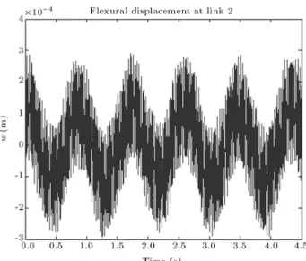
Figure 5. Lateral deection at the tip of link 2.

Figure 6. Axial deection at the tip of link 2.

Figure 7. Endpoint trajectory viewed in global coordinate system.

elastic nonlinear formulations to illustrate the perfor-mance of the simulation and the eect of the geometric nonlinearity. In the second test, a robot manipulator with elastic links is considered. The end-eector and its load must track a straight line with a predened speed. In the third test, MADL is found for a exible robot manipulator in which the end-eector must move along a circular path. In the last two cases, the mobile base of the manipulator moves along a straight line at a constant speed.

1R Planar Rotating Flexible Manipulator In this section, the dynamic characteristics of the rotat-ing exible manipulator are studied through numerical simulations (Figure 8), for the computational eciency of geometric nonlinearity at high speed is comparable to that of a linear formulation. The properties of the exible manipulator are the same as those in [10], and are given as follows:

The length: L = 8 m;

The cross section area: A = 7:3 10 5 _m2_;

The second moment of area: I = 8:218 10 9 _m4_;

The mass density: = 2:7667 103 _kg/m2_;

The Young's modulus of material: E = 68:95 GPa. The rotating exible manipulator spun-up according to a motion law is dened by:

(t)=

!s

Ts

" t2

2

+

Ts

2 2

cos

2t Ts

1

# ; (29) where !s and Ts are the rating angular velocity and

start-up time, respectively. In this simulation, Ts =

15 s and the rotation speed, !s, is varied from 0.1 ras/s

to 2.5 rad/s.

Figures 9 and 10 show the deection obtained at an angular velocity, !s, of 1 and 2.5 rad/s,

re-spectively. As can be seen, elastic displacements are small at a small angular velocity so both the linear

Figure 8. 1R planar rotating exible manipulator.

Figure 9. Deection on the link end with !s= 0:1 rad/s.

Figure 10. Deection on the beam end with !s= 2:5

rad/s.

and the nonlinear formulation lead to the same solution (Figure 9). As shown in Figure 10, when the angular velocity is raised to 2:5 rad/s, the results provided by the simulation, not including the eects of geometric elastic nonlinearity, are divergent and inconsistent with the actual physical response. This is the result of an increase in the rotation speed increasing both centrifugal axial forces and the displacement amplitude through deection of the link.

MADL of a Flexible Mobile Manipulator with a Linear Path

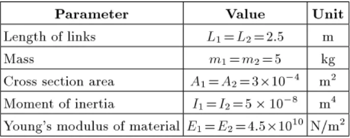
This simulation study is performed to investigate the eciency of the procedure presented in Figure 11 for computing the maximum allowable load of a mobile manipulator. All required parameters are given in Table 1. As mentioned earlier, the path of the

end-Figure 11. Schematic of robot and the desired path of end-eector.

Table 1. Simulation of parameters.

Parameter Value Unit Length of links L1=L2=2:5 m

Mass m1=m2=5 kg

Cross section area A1=A2=310 4 m2

Moment of inertia I1=I2=5 10 8 m4

Young's modulus of material E1=E2=4:51010 N/m2

eector and its payload is linear, which starts from point x1 = 0 and y1 = 3:5 m and ends at a point

with coordinate x2= 1:72 m and y2= 4:4 m.

The velocity prole of the end-eector is as below: 8

> < > :

v = at 0 t T=4

v = vmax T=4 t 3T=4

v = at 3T=4 t T

(30) A linear path is planned for the vehicle, which starts from the origin and ends at xb2= 0:99 m and yb2= 0:26

m, with the velocity of Vb = 0:2t. The obtained path

of the end-eector, considering link exibility is shown in Figure 12 in comparison with the desired path. Also, the joint angles of rigid and exible link states are shown in Figures 13 and 14. The corresponding applied torques to the manipulator actuators are shown in Figures 15 and 16.

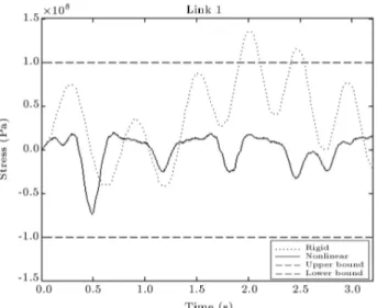
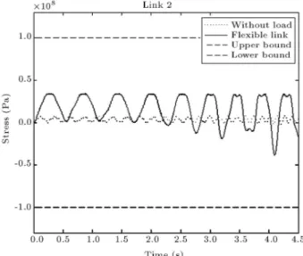
Links can be regarded as cantilevers. Thus, the maximal dynamic stress should occur close to the joints. The numerical simulation results show that the maximal dynamic stresses of links change signicantly with the load. As shown in Figures 17 and 18, the

Figure 12. The desired and the actual load path.

Figure 13. Joint responses of 1for rigid and exible

links.

Figure 14. Angular positions of 2 for rigid and exible

Figure 15. Actuator torque at the rst joint against torque bounds.

Figure 16. Actuator torque at the second joint.

Figure 17. Maximal dynamic stress of exible link 1 against stress bounds.

maximal dynamic stress values uctuate frequently and arise to the admissible stress with maximum load.

The relation between the magnitude of residual vibration and the amount of payload is concluded. As can be seen, the exibility of the link and adding the payload will non-linearily increase the amplitude of the residual vibrations. The variation trend of RRV, with respect to payload mass for a exible link manipulator, is shown in Figure 19. This non-uniform increasing trend of RRV is because of displacement and velocity errors at the nal time. Depending on the initial conditions, the magnitude of the residual vibration's amplitude may vary. With these descriptions, to estimate the residual vibration amplitude in terms of the payload value, a tangent line to the maximum value of RRV can be considered as shown in Figure 19. This line can be used for considering the residual

Figure 18. Maximal dynamic stress of exible link 2 during the linear path.

Figure 19. Maximum residual vibration versus payloads in the linear path.

vibration as a constraint in computing the maximum payload.

Now, the MADL of the robot of the previous section can be computed. The permissible error bound for the end-eector motion around the desired path is Rp = 6 cm, and at the end point is Rrv = 16:5 cm.

Both actuators of the robot are considered to be the same, with Ts = 230 N.m and !n1 = 10 rad/s and

allowable stresses of the links are considered to be the same with Us= 100 MPa. The MADL, by imposing all

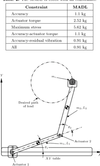
constraints, are found and given in Table 2. Therefore, the maximum allowable dynamic load of the robot, considering all constraints, is calculated to be 0.91 kg for the given linear path.

MADL of a Flexible Mobile Manipulator with a Circular Path

In this simulation, the computation of the MADL for a two-link planar manipulator mounted on an XY table (Figure 20) is presented. The link parameters

Table 2. The MADL of robot with all constraints. Constraint MADL Accuracy 1.1 kg Actuator torque 2.52 kg Maximum stress 5.62 kg Accuracy-actuator torque 1.1 kg Accuracy-residual vibration 0.91 kg

All 0.91 kg

Figure 20. Schematic of exible link planar manipulator with the circular path.

and inertia properties of the manipulator were given in Table 3. In the inertial reference frame, the XY table is capable of moving 1000 mm along the X-axis. Base velocity is Vx= 0:1t. Also, it is assumed that the load

must move along a circular path. The centre of the circular path coordinates with radius r = 50 cm is at xc= 1 m and yc= 1 m with its origin at the lower-left

corner of the XY table (Figure 21).

The obtained path which is tracked by the exible robot manipulator is compared with the desired path in Figure 21. In this case, the permissible error bound for the end-eector motion around the desired path is Rp = 6 cm, and at the end point is Rrv =

3 cm.

Both actuators of the robot and allowable stresses are considered to be the same with Ts = 170 N.m,

!nl = 5 rad/s and Us = 100 MPa, respectively. The

corresponding applied torques to each actuator are shown in Figures 22 and 23. The maximal dynamic stresses are shown in Figures 24 and 25 and the variation trend of RRV with respect to payload mass for the exible link manipulator with the circular path is shown in Figure 26. The MADL, by imposing imposing all constraints, is found and given in Table 4. Therefore, the maximum allowable dynamic load of the

Table 3. Parameters of two-link planar exible manipulator.

Parameter Value Unit Length of links L1=L2=1:2 m

Mass m1=M2=2:4 kg

Cross section area A1=A2=3 10 4 m2

Moment of inertia I1=I2=5 10 8 m4

Young's modulus of material E1=E2=4:51010 N/m2

Figure 21. Desired and actual trajectory in the circular path.

Figure 22. Variation of rst joint torque with time within upper and lower acceptable boundaries.

Figure 23. Applied torques of the second motor.

Figure 24. Maximum dynamic stress of exible link 1 during the circular path.

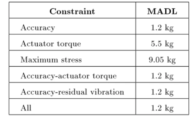
robot considering all constraints is found to be 1.2 kg for the given trajectory.

The results depicted the importance of all con-straints. According to accuracy and tracking, they show which one would be the main one. The simulation results indicate that the main reason for manipulator deviation is its major link's exibility.

CONCLUSIONS

The main objective of this study was formulating and determining the Maximum Allowable Dynamic Load (MADL) for geometrically nonlinear exible-link manipulators with a pre-dened trajectory, using the nite element method. A complete dynamic model is considered to characterize the motion of a compliant link capable of large deection. The MADL was

Figure 25. Maximal dynamic stress of exible link 2 during the circular path.

Table 4. Maximum allowable dynamic load in circular path.

Constraint MADL Accuracy 1.2 kg Actuator torque 5.5 kg Maximum stress 9.05 kg Accuracy-actuator torque 1.2 kg Accuracy-residual vibration 1.2 kg

All 1.2 kg

achieved by imposing actuator torque capacity, end ef-fector accuracy, maximum stress and residual vibration constraints to the problem formulation. In simulation studies, a two-link planar manipulator mounted on a mobile base was considered for carrying a load in two-test cases. Numerical results obtained indicate that the inclusion of geometric elastic nonlinearities in the mathematical model leads to the development of a new geometrically nonlinear stiness matrix whose neglect will aect the overall behavior of the robot. The results of the case study show that the allowable load is variable along the given trajectory. In addition, the formulation is more stable and ecient than most alternatives and has the added advantage of being able to calculate residual vibration and a new eective constraint, as \the dynamic stress constraint of links". Therefore, the permissible error bound for constraints in large deformation is sensitive in calculating the MADL.

NOMENCLATURE

1; 2 angular displacements of joints 1 & 2

L1; L2 total lengths of links 1 and 2

m1; m2 total mass of links 1 and 2

I1; I2 moment of inertia of links 1 and 2

A1; A2 cross section of links 1 and 2

E1; E2 Young's modulus of links 1 and 2

u2i axial displacement at common junction

of elements `i' and `i + 1' of link 1 v2i exural displacement at common

junction of elements `i' and `i + 1' of link 1

2i exural slope at common junction of

elements `i' and `i + 1' of link 1 n1; n2 number of elements of links 1 and 2

qi generalized coordinates

M1; M2 generalized inertia matrices of links 1

and 2

K1; K2 stiness matrices of links 1 and 2

r(x) vector from the origin to a point on element

rfx; rfy the position of the goal point from

exible robot

p2i axial displacement at common junction

of elements `i' and `i + 1' of link 2 w2i exural displacement at common

junction of elements `i' and `i + 1' of link 2

'2i exural slope at common junction of

elements `i' and `i + 1' of link 2 REFERENCES

1. Al-Bedoor, B.O. and Hamdan, M.N. \Geometrically non-linear dynamic model of a rotating exible arm", Journal of Sound and Vibration, 240(1), pp. 59-72 (2001).

2. Liu, J.Y. and Hong, J.Z. \Geometric stiening of exi-ble link system with large overall motion", Computers and Structures, 81, pp. 2829-2841 (2003).

3. Book, W.J. \Recursive Lagrangian dynamics of exible manipulator arms", Int. J. Robotics Res., 3(3), pp. 87-101 (1984).

4. Meghdari, A. \A variational approach for modeling exibility eects in manipulator arms", Robotica, 9, pp. 213-217 (1991).

5. Damaren, C. and Sharf, L. \Simulation of exible-link manipulators with inertia and geometric nonlineari-ties", ASME J. Dyn. Syst., Meas., Control, 117, pp. 74-87 (1995).

6. Zhang, C.X. and Yu, Y.Q. \Dynamic analysis of planar cooperative manipulators with link exibility", ASME J. of Dyn. Sys. and Control, 126, pp. 442-448 (2004). 7. Book, W.J. \Modeling, design, and control of exible manipulator arms: a tutorial review", Proc. of the IEEE Conf. on Decision and Control, pp. 500-506 (1990).

8. Meghdari, A. and Fahimi, F. \On the rst-order decoupling of dynamical equations of motion for elastic multibody systems as applied to a two-link exible manipulator", Multibody System Dynamics, 5, pp. 1-20 (2001).

9. Absy, H.E.L. and Shabana, A.A. \Geometric stiness and stability of rigid body modes", J. Sound Vib., 207(4), pp. 465-496 (1997).

10. Mayo, J. and Dominguez, J. \A nite element geo-metrically nonlinear dynamic formulation of exible multibody systems using a new displacements repre-sentation", Vibration and Acoustics, ASME, 119, pp. 573-581 (1997).

11. Bakr, E.M. \Dynamic analysis of geometrically non-linear robot manipulators", Nonnon-linear Dynamics, 11, pp. 329-346 (1996).

12. Shaker, M.C. and Ghosal, A. \Nonlinear modeling of exible manipulators using non-dimensional vari-ables", ASME, J. of Computer and Nonlinear Dyn., 1, pp. 123-134 (2006).

13. Pratiher, B. and Dwivedy, S.K. \Non-linear dynamics of a exible single link Cartesian manipulator", Int. J. of Non-Linear Mechanics, 42, pp. 1062-1073 (2007). 14. Zohoor, H. and Khorsandijou, S.A.M. \Dynamic

model of a ying manipulator with two highly exible links", Applied Mathematical Modelling, 32, pp. 2117-2132 (2008).

15. Wang, L.T. and Ravani, B. \Dynamic load carrying capacity of mechanical manipulators - Part I: Problem formulation", ASME, J. of Dyn. Sys., Meas. & Cont., 110, pp. 46-52 (1988).

16. Korayem, M.H. and Ghariblu, H. \Maximum allowable load on wheeled mobile manipulators imposing redun-dancy constraints", J. of Rob. & Auto. Sys., 44(2), pp. 151-159 (2003).

17. Yue, S. and Tso, S.K. \Maximum dynamic payload trajectory for exible robot manipulators with kine-matic redundancy", Mech. Mach. Theory, 36, pp. 785-800 (2001).

18. Korayem, M.H. and Shokri, M. \Maximum dynamic load carrying capacity of a 6 ups-stewart platform manipulator", Scientia Iranica, 15(1), pp. 131-143 (2008).

19. Korayem, M.H. and Heidari, A. \Maximum allowable

dynamic load of exible mobile manipulators using nite element approach", Adv. Manuf. & Tech., 36, pp. 606-617 (2007).

20. Zhaocai, D. \Analysis of dynamic stress and fatigue property of exible robot", Proc. of IEEE Int. Conf. on Rob. and Bio, pp. 1351-1355 (2006).

21. Korayem, M.H., Nikoobin, A. and Heidari, A. \The eect of payload variation on the residual vibration of exible manipulators at the end of the given path", Scientica Iranica, Transaction B, 16(4), pp. 332-343 (2009).

22. Abe, A. \Trajectory planning for residual vibration suppression of a two-link rigid-exible manipulator considering large deformation", Mech. Mach. Theory, 44, pp. 1627-1639 (2009).

23. Criseld, M.A., Nonlinear Finite Element Analysis of Solids and Structures, John Wiley & Sons, England (2001).

24. Robinett III, R.D., Feddema, J., Eisler, G.R., Dohrmann, C., Parker, G.G., Wilson, D.G. and Stokes, D., Flexible Robot Dynamics and Controls, IFSR Inter-national Series on Systems Science and Engineering, 19, New York, Plenum Publishers (2002).