ISSN: 2322-1666 print/2251-8436 online
BANDWIDTH SIMULATION AS A MONTE CARLO QUEUING SYSTEM
A. HADIAN, M. BAGHERIAN, B. F. VAGARGAHI, S. S. AYAT
Abstract. One of the issues raised in cloud computing is the dat-acenter locating problem and one of the effective factors in design-ing data center locations is amount of data volume and referrals to it. This depends on the number of customers or users who are going to use that data center, which is a probable issue. In this paper, the bandwidth simulation is described by considering the bandwidth system as a queuing system and simulating it by Monte Carlo method. We explain how to simulate the bandwidth con-sumption in different static and dynamic simulation states for a real computer system and we show that the bandwidth required at an Endpoint in cloud computing can be calculated with different Gamma distribution parameters.
Key Words: Cloud Computing, Monte Carlo Simulation, Bandwidth simulation. 2010 Mathematics Subject Classification:Primary: 13A15; Secondary: 13F30, 13G05.
1. Introduction
The concept of cloud computing is a combination of different sized networks and distributed data computing, which today has become one of the topics discussed in science and research as well as in commerce. The concept of cloud computing is not generally a new discussion, but because of the growth and maturity of the methods that have been proposed in recent years, it has covered complex debates on parallel processing and network computing. In fact, cloud computing can be Received: 15 January 2018, Accepted: 21 January 2018. Communicated by A. Yousefian Darani;
∗Address correspondence to A. Hadian; E-mail: [email protected]. c
2018 University of Mohaghegh Ardabili. 50
viewed from two perspectives, cloud computing and content-based net-works, which include incorporating or sharing information resources in the field of information technology, including different type of computer file such as video, audio, image or any type of data that can be stored [1, 3, 4]. One of the primary requirements for designing data centers in cloud networks is to calculate the bandwidth of consumers. In this paper, we intend to calculate the bandwidth required by a system as the basis of computing in cloud computing with a systemic look at the con-cept of bandwidth and its simulation. One of the issues for institutions and corporations is the location in the design of their data centers. This will require statistical data for estimate the bandwidth of the consumer. To it, we consider bandwidth usage as a system and simulate this sys-tem. In order to do this, we consider a computer system that receives three types of data. In order to understand the broadband system in cloud computing, we need to have to introduction of basic concepts of information theory, which we will discuss below, and then simulate the system and calculate it.
2. The basic concepts and how to simulate the problem Mathematical theory of optimal sending, receiving and storing data and information is called information theory. In this theory, Claude Shannon has examined the way of modeling the problem sending infor-mation in telecommunication channels, and provides a complete model for mathematical modeling of the source of information, the channel of information transmission and retrieval. The two most important results, known as Shannon’s theorems, are: 1. The minimum rate to which we can limit the rate of information compressing of a random source of in-formation equal to the entropy of that source. In other words, we can’t send the sequence of the output from one information source with less than the entropy of that source. 2. The maximum rate that can be sent on a telecommunication channel in a way that is capable of detecting in-formation at the destination with the probability of an acceptable error (low error), is a fixed and specific value of channel, which it is channel capacity. Sending at a rate higher than the capacity of a channel on it leads to error [2,5].
Therefore, information theory is examined from three perspectives: 1. Storage and retrieval of information 2. Processing of information 3. Information transfer, which are referred to the basis of cloud computing. So If y is a variable of volume and t is a time variable, we consider
respectively units of speed and volume measurement bits per second which is shown with bps and byte with B. The relationship between the time of data transfer and the volume of information is always a constant value and equals 0.125. In mathematics, means
(2.1) y=f(a, t) = 0.125at⇒t=f−1(a, y) = 8y/a
In which a bandwidth is given. For example, if you have a 40MB file and want to calculate the download time with a 200Kbps connection, this time ist= (40×8×40×220)/(200×210) = 1638.4 seconds, that is, about 27 minutes. Or if we want to see how much of this file has been downloaded at the same speed after 10 minutes, we have:
y= 0.125×200×210×10×60 = 15000KB ≈14.65M B
With this description, the technical form of the problem is clear. In other words, if we want to connect a computer to a server, the router in the first hub should provide service with appropriate bandwidth to the user. Each click is considered an event, and because every click that re-quest a site outside of the local network, go to the router and the router checks and leads it, so the router should be considered for simulation. Here, we should pay attention to the click and bandwidth relationship. Because one single click can request a download or a link in a site that is already open, so downloading is directly depended on the size of the file which user has requested and depending on the bandwidth it can take a long time. But one Click in the page of a site, can be opened in less than one second. Regarding this topic, there is the possibility of opening or requesting four categories of sites on the computer.
Category 1: The sites related to the user’s working servers. Category 2: Non-working sites such as news sites and so on.
Category 3: software update sites installed on the computer system Category 4: Sites or servers that are out of reach in any reason and can’t be accessed. Before designing the problem model, several point is needed to be expressed:
1. regarding to the formula (2.1) , the time in the desired system can be represented by volume. This means that the simulation time can be expressed with the certain size of information volume, and vice versa. 2. The probability that the user will request a particular category of in-formation at a particular moment is not clear, which means that the user can open several pages of the web at the same time and click on different pages, so concurrency Clicks on the user’s computer are not specified and this issue is identified on the router. Therefore, the probability that the
user requests from the router, first, second or third category is consider PC1, PC2 and PC3 respectively. And with the probabilityPC4 the site is
not available for demand.
3.The client in this system means user requests or clicks, and the server is the speed or bandwidth that each click needs. That if the bandwidth is full it waits for the request, otherwise it will lead to the target site and exchange information.
4. there are two types of processing by the server in this problem, the first service identifies the packet path, which due to the speed of exist-ing routers processors and the concepts and routexist-ing tables available in the current routers, very limited time expends to do this service. And so the first service processing time is negligible and we neglect it. But the second, third, and fourth services is meant when communication is made, and the server and the client are connected. The occupancy of these services means the time of downloading the page or opening the requested file (according to formula (2.1))
5. During simulation to determine how much bandwidth we need to configure for each category of sites. At first, to find the distribution of probabilities for each category, we assume that the available bandwidth is free and available to all categories.
Given these points, the problem can be expressed as a system. Systematic Definition Problem: In a server (a communication channel) four categories of information are exchanged. This information includes requests from users to the sites in these four categories. IfPCi is the probability that the request is requested from the i-th category, ( i=1..4 and P4i=1Pci = 1). The total bandwidth of this server at the beginning of this simulation is 10 Mbps, we simulate this system for seven hours, so that in the end, it would be clear that each type of in-formation will occupy how much volume of total bandwidth during this time period.
To solve the problem according to formula (2.1), the probability of each category equals to the volume of data transmitted in each case, divided by the total of data transmitted. Therefore, the system is con-sidered as a queue. The pseudocode of simulate this system as follows. In this algorithm, the S variable is used to indicate the status of the service providers and Q is the number of people in the queues.
Algorithm: Generic pseudocode to simulate the problem Start {
Q1 = Q2 = Q3 = Q4 = Q5 = y = 0; S1 = S2 = S3 = S4 = S5 = 0;
TBL(1)=0; // The time of first click the size of first download is zero. TBL(2,3,4) = ST+1;
While ( The time of simulation is not completed ) {
y = minTBL(1,2,3,4); k = minIndex;
switch(k) {
case 1 : Routepacket(); break; case 2 : Endp2(); break; case 3 : Endp3(); break; case 4 : Endp4(); break; case 5 : Endp5(); break;
} } }
Endp2,3,4() {
if (Q(2,3,4,5)==0) {
S(2,3,4,5)=0; Time(2,3,4,5)=ST+1;
}
else{
Q(2,3,4,5)=Q(2,3,4,5)-1;
TBL(3,4,5) = y + Size of packets downloaded from Class 1,2,3,4.
} }
Routepacket() {
if ( bandwidth is full) Q1 = Q1 + 1;
else {
if( Rand() < Pci1 )
if (S2==0) {
S2 = 1;
TBL(2) = y + Size of packets downloaded from Class 1;
} else
Q2=Q2+1;
else if ( Rand() < Pci2 )
if (S3==0){
S3 = 1;
TBL(3) = y + Size of packets downloaded from Class 2;
} else Q3=Q3+1; else if ( Rand() < Pci3 )
if (S4==0){
S4 = 1;
TBL(4) = y + Size of packets downloaded from Class 3;
} else Q4=Q4+1; else if(S5==0){
S5 = 1;
TBL(5) = y + Size of packets downloaded from Class 4;
} else Q5=Q5+1;
} // end of first else.
Table 1. The statistics of the problem data
Category C1 C2 C3 C4
Number of messages 51403 29760 43287 10822 Number of requests or clicks 1542 893 1299 324 The amount of downloaded data 311 852 114 73
Pci 0.38 0.22 0.32 0.08
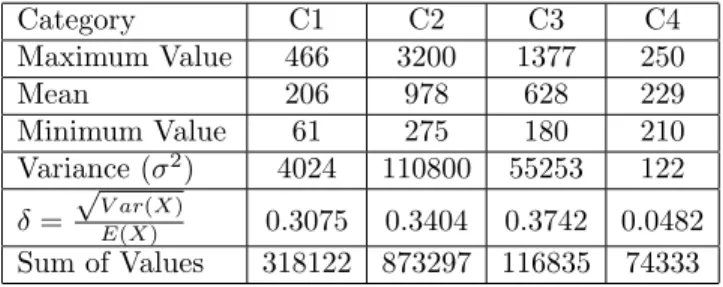
Table 2. Statistics on problem data according to KB
Category C1 C2 C3 C4
Maximum Value 466 3200 1377 250
Mean 206 978 628 229
Minimum Value 61 275 180 210 Variance (σ2) 4024 110800 55253 122 δ=
√
V ar(X)
E(X) 0.3075 0.3404 0.3742 0.0482 Sum of Values 318122 873297 116835 74333
As it is known in pseudocodes, variables such asPci and the amount of data
transmitted in each connection are unclear and should check by the study of a real network.
3. Analysis of problem data and numerical results
To compile the prototype data for simulation, we considered a computer system. The router on that network is a MikroTik. Kiwi product is used to record the clicked links on the computer. The analyzed data obtained from Sawmill software. Here, the computer’s data obtained at seven hours of time, and results saved in the file about 24MB by recording 135,272 system events. So in this simulation system, the arrivals to the router or the first queue is an exponential distribute with an average of 6 seconds. According to these data, after data scrutiny, the data is obtained as shown in table 1.
According to the data in the table 1, we find that the bandwidth consumed in these seven hours is 1350MB. The data obtained by MATLAB R2016a software has been analyzed. Table 2 shows the obtained statistics. To estimate the statistical distribution of data, there are ways, such as the use of point statistics
δ, histogram diagrams and probabilistic maps or the Maximum Likelihood Estimator (MLE) method [7,8].
Given the positive data and the histogram, also, the value of δobtained in Table 2 is a few points about the guessing of the statistical distribution of the data:
1. Since the time component in this problem and the time are continuous, we assume continuous distributions.
2. Because the data is positive, distributions that have a negative domain, such as normal distribution, are not considered.
3. Given the proximity of the intervals in the fourth category’s histogram, can guess the uniform distribution in [210,250].
4. To guess distribution of the first to third categories, considering the category’s histogram, since δ < 1, one can guess the chi-square and gamma distributions with the parameterα > 1. Therefore, according to the table 1 and 2 and according to the data values, the distribution of the first category is a chi square distribution with 20 degrees of freedom, the distribution of the second category is the Gamma Ga(α, β)=Ga (10,80) and the distribution of the third category is Ga(α, β)=Ga(8,75) distribution. To prove it we can use statistical tests. This was done with MATLAB. With this in mind, the initial guess about distributions is close to reality, and so the distribution of each of the four categories of information requested is as follows: The first category’s distribution is Ga(10.62,19.43), the second category has Ga(10.29,95.02) dis-tribution, the third category has the Ga(7.33,85.71) and distribution of final category is U(210,250). Since the Chi square distribution is the same Gamma distribution with v
2 degrees of freedom, we consider the Gamma distribution for this problem.
4. Problem simulation
Static simulation: Because the bandwidth in this problem is high, accord-ing to equation (2.1), each kilobyte is transmitted at 0.0001 seconds, and on the other hand, every 6 seconds, one click, with a maximum volume of 1024K, is passed. Therefore, according to the contents of the previous sections, it is possi-ble to write the propossi-blem of static simulation in the MATLAB programming[8]. We know that the Gamma distribution of the density function is (4.1): (4.1) f(x) =Ga(α, β) = 1
βαΓ(α)x
α−1e−x/β =kxα−1e−βx
To generate a random number, we use the Gamma distribution into a rejection method. To do this, we define the function g at the relation(4.2).
(4.2) g(x) = 1
βαe α−2
β x
Then we should find the maximum value of the ratio f to g. To do this we consider the function h, which is the ratio of these two functions.
h(x) = f(x)
g(x) =
kxα−1e−x β
1
βαe α−2
β x
=β
αkxα−1e−x β
eα−β2x
If we set derivative h to zero, the value of c is obtained as follows:
c=h(β) =βαkβα−1e1−α= β α
βαΓ(α)β
α−1e1−α= β
α−1e1−α Γ(α) By obtaining the constant c, we define the functionl(x) as follows.
l(x) = f(x)
cg(x) = (
x βe
1−x β)α−1
On the other hand, the inverse of the function g is equal to:
g−1(x) = β
α−2(αlnβ+lnx)
Therefore, the rejection algorithm to find a random variable of Gamma dis-tribution will be as follows:
Rejection Algorithm generate random number with Γ distribution
1. Produceu1∼U(0,1) and sety=αβ−2(αlnβ+lnu1). 2. Produceu2∼U(0,1).
3. Ifu2< l(y) then set X=Y and stop, else go to 1.
After simulating the problem for 1 hour, we find that the first category of data occupies 1% of the total bandwidth. The second category of data occu-pies 3% of the total bandwidth. The third category of data occuoccu-pies 3% of the total bandwidth. The fourth category of data occupies 0.2% of the total bandwidth. According to relation (2.1) , each category of data is occupied by 36, 108, 108, and 7 seconds, respectively. In other words, within one clock, a maximum of 6% of the total capacity of a broadband provider is used. The minimum bandwidth for this issue, which means the minimum amount of each category that you want to receive at a time, is 770Kbps and the maximum is about 3.8Mbps. The total amount of information exchanged in this one hour is 293MB.
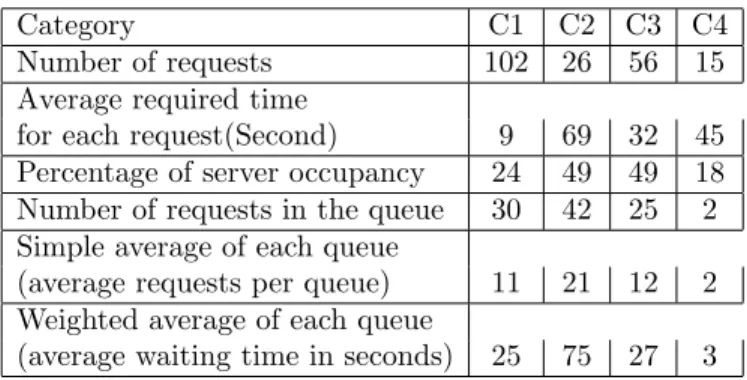
Dynamic simulation: If we want to simulate the same problem with 512Kbps bandwidth so because the speed of the server is less than the demand for the client, the queue and waiting times for some requests will certainly arise. Therefore, the requests queue should be considered for it. According to formula (2.1), we express the problem with time. It needs to be explained that because the bandwidth is limited and at any time each request classifies into its category, then we need to divide the bandwidth by the percentage of usage per category. For example, the first category will need bandwidth of 0.36×512 = 194.6Kbps. Table 3 shows the outputs simulating. As shown in this table, due to bandwidth limitation for all of category is formed a queue
Table 3. Dynamic Simulation Results
Category C1 C2 C3 C4
Number of requests 102 26 56 15 Average required time
for each request(Second) 9 69 32 45 Percentage of server occupancy 24 49 49 18 Number of requests in the queue 30 42 25 2 Simple average of each queue
(average requests per queue) 11 21 12 2 Weighted average of each queue
(average waiting time in seconds) 25 75 27 3
and the categories occupy 24, 49, 49, and 18 percent of the server time, respec-tively. Also, on average, each request in each queue is waited 25, 75, 27 and 3 seconds respectively in their queue.
5. Conclusion
In designing a cloud computing system, one of the major issues is the location of data centers, which needs to estimate the bandwidth required. This paper presents a method for estimating the bandwidth of a computer by simulation. Studies have not been done on this so far. And in this article, the client system was studied, and we will study the bandwidth server system to continue the work.
References
[1] T. Erl, R. Puttini, Z. Mahmood, Cloud Computing, Concepts. Technology and Architecture, 1st edn. Prentice Hall Press, Upper Saddle River, (2013).
[2] Jones, Garth A, Information and coding theory, Journal of Springer, (2000) ISBN:978-1-4471-0361-5
[3] Krzysztof Walkowiak,Modeling and Optimization of Cloud-Ready and
Content-Oriented Networks, Studies in Systems, Decision and Control 56, Springer
(2016),ISBN: 978-3-319-30309-3
[4] M. Klinkowski, K. Walkowiak,On the advantages of elastic optical networks for provisioning of cloud computing traffic, IEEE Network,(2013), 27(6), p4451 [5] G. Held, A Practical Guide to Content Delivery Networks, Auerbach
Publica-tions,(2005), Boston
[6] S. Tarkoma,Overlay Networks: Toward Information Networking, 1st edn. Auer-bach Publications,(2010) Boston
[7] M. Ross, Shelon, , A course in simulation, Prentice, Hall College Div, (June 1990) ISBN-13: 978-0024038913
[8] Y. Rubinstein, Reuven,Simulation and Monte Carlo method, Trancelated by B. Fathi, Guilan university Pulisher,(2013), ISBN: 978-600-153-064-7
Ali Hadian
Phd Student, Department of Applied Mathematics, Faculty of Mathematical Sciences, University of Campus2,University of Guilan, P.O.Box 84475 - 41447, Rasht, Iran Email: [email protected]
Mehri Bagheian
Department of Applied Mathematics, Faculty of Mathematical Sciences, University of Campus2,University of Guilan, P.O.Box 41996 - 13776, Rasht, Iran
Behrouz Fathi Vajargah
Department of Applied Mathematics, Faculty of Mathematical Sciences, University of Campus2,University of Guilan, P.O.Box 41996 - 13776, Rasht, Iran
Sayyed Saeid Ayat
Department of Computer Engineering and Information Technology, Faculty of Com-puter Engineering and Information Technology, University of Najafabad Payame Noor,P.O.Box 85156-43144 Najafabad, Isfahan, Iran