Research Note
Variable, Step-Size, Block Normalized,
Least Mean, Square Adaptive
Filter: A Unied Framework
M. Shams Esfand Abadi
1, S.Z. Moussavi
and A. Mahlooji Far
2Employing a recently introduced framework, within which a large number of classical and modern adaptive lter algorithms can be viewed as special cases, a generic, variable step-size adaptive lter has been presented. Variable Step-Size (VSS) Normalized Least Mean Square (VSSNLMS) and VSS Ane Projection Algorithms (VSSAPA) are particular examples of adaptive algorithms covered by this generic variable step-size adaptive lter. In this paper, the new VSS Block Normalized Least Mean Square (VSSBNLMS) adaptive lter algorithm is introduced, based on the generic VSS adaptive lter. The proposed algorithm shows the higher convergence rate and lower steady-state mean square error compared to the ordinary BNLMS algorithm.
INTRODUCTION
Adaptive ltering has been, and still is, an area of active research that plays an important role in an ever increasing number of applications, such as noise cancellation, channel estimation, channel equalization and acoustic echo cancellation. The least mean square (LMS) and its normalized version (NLMS) are the workhorses of adaptive ltering. In the presence of colored input signals, the LMS and the NLMS algo-rithms have extremely slow convergence rates. To solve this problem, a number of adaptive ltering structures, based on ane subspace projections [1,2] and multirate techniques, have been proposed in the literature [3-5]. In all these algorithms, the selected xed step-size can change the convergence rate and the steady-state mean square error. By optimally selecting the step-size, during the adaptation, one can obtain the both fast convergence rate and low steady-state Mean Square Error (MSE). Important examples of the two new Variable Step-Size (VSS) versions of the NLMS and the
1. Department of Electrical Engineering, Shahid Rajaee Teacher Training University, Tehran, I.R. Iran. *. Corresponding Author, Department of Electrical
Engi-neering, Shahid Rajaee Teacher Training University, Tehran, I.R. Iran.
2. Department of Electrical Engineering, Tarbiat Modarres University, Tehran, I.R. Iran.
Ane Projection (AP) algorithm can be found in [6]. In [7], the generic adaptive lter, based on the weighted, estimated Wiener-Hopf equation, is proposed. The LMS and the NLMS adaptive algorithms, the family of Ane Projection Algo-rithms (APA), the Transform Domain Adaptive Fil-ters (TDAF) [8] and the Pradhan Reddy Subband Adaptive Filters (PRSAF) [9] are the particular ex-amples that can be covered with this generic adaptive lter.
The objective, in this paper, is rstly to show that the generic adaptive lter proposed in [7] can cover the Block LMS (BLMS) and the Block Normalized LMS (BNLMS) adaptive lter algorithms. Secondly, based on the generic adaptive lter, the generic variable step-size update equation is developed. The VSSNLMS and VSSAPA of [6] can be easily derived from this generic variable step-size adaptive lter. The following proceeds by presenting the VSS version of the BNLMS adaptive lter, named the VSSBNLMS, which is char-acterized by the fast convergence speed and reduced steady-state MSE, when compared to the ordinary BNLMS adaptive lter algorithm.
The paper is organized as follows: In the following section, the generic variable step-size update equation, forming the basis of the development of the VSS-BNLMS, is introduced. Subsequently, the VSSBNLMS algorithm will be presented. In the next section, the computational complexity of the BNLMS and
VSS-BNLMS is calculated and compared. Finally, before concluding the paper, the advantages of the algorithms are demonstrated by presenting several experimental results.
GENERIC VARIABLE STEP-SIZE UPDATE EQUATION
The generic lter vector update equation at the center of this analysis can be stated as [10-12]:
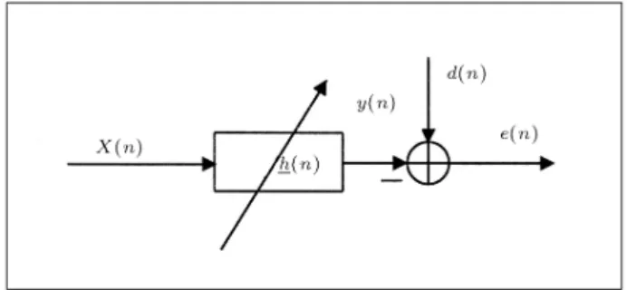
h(n + 1) = h(n) + X(n)W (n)e(n): (1) A notation is used, based on the adaptive ltering setup shown in Figure 1 and explained in Table 1.
Note that all vectors are columns, unless explicitly transposed through the superscript, T , notation. For more details, please refer to [10-12].
An important goal for all adaptive lters is the rapid convergence to an accurate solution of the Wiener-Hopf equation in a stationary environment. The Wiener-Hopf equation is:
Rht= r; (2)
where ht is the unknown true lter vector, R is the autocorrelation matrix of the lter input signal, R = Efx(n)xT(n)g, and r is the crosscorrelation vector
Figure 1. Adaptive lter setup.
dened by r = Efx(n)d(n)g:d(n) is commonly referred to as the desired signal that arises from the linear model, d(n) = xT(n)h
t + v(n), where v(n) is the
measurement noise. Since one cannot expect the exact knowledge of R and r of Equation 2 and, because it is reasonable to assume those quantities to be time dependent, it makes sense to formulate the adaptive ltering problem as the problem of nding the time dependent solution, h(n), to:
^
R(n)h(n) = ^r(n); (3)
where ^R(n) and ^r(n) denote estimates of the correla-tion quantities of Equacorrela-tion 2. By dening the M K data matrix, as follows:
X(n)=[x(n); x(n 1); x(n 2); ; x(n K+1)]; (4) and, being given some K K full rank symmetric weighting matrix W (n), one could reasonably state the estimated Wiener-Hopf equation (Equation 3) as:
X(n)W (n)XT(n)h(n) = X(n)W (n)d(n); (5)
where d(n) is a K 1 vector of desired signal samples, dened as:
d(n)=[d(n); d(n 1); d(n 2); ; d(n K+1)]T; (6)
that can be obtained from the following equation: d(n) = XT(n)h
t+ v(n); (7)
where v(n) = [v(n); v(n 1); ; v(n K + 1)]T is the
measurement noise vector. It is noticed that, if W (n) = I, where I is the identity matrix, the estimates used are standard sample estimates of the correlation quantities involved. The larger the value of K is selected, the better estimates one would expect. Selecting W (n) dierent from the identity matrix makes it possible to
Table 1. Explanation of notation.
h(n) Length M column vector of lter coecients to be adjusted at each time instant n x(n) Length M vector of input signal samples to adaptive lter,
x(n) = [x(n); x(n 1); ; x(n M + 1)]T
e(n) Length K vector of error samples, e(n) = [e(n); e(n 1); ; e(n K + 1)]T
X(n) M K signal matrix whose columns are given by: [x(n); x(n 1); ; x(n K + 1)]
W (n) K K symmetric weighting matrix Step-size
use weighted estimates of the correlation quantities. For the case when W (n) = [XT(n)X(n)] 1, or some
function of this quantity, it is common to refer to the associated estimates as the data normalized estimates. Applying a stationary iterative linear equation solver [13] to Equation 5 entails a splitting of the coecient matrix, X(n)W (n)XT(n):
X(n)W (n)XT(n) = (:I) 1 [(:I) 1
X(n)W (n)XT(n)]; (8)
where is step-size and I is the identity matrix, therefore, :I is a M M full rank matrix. Fur-thermore, performing only one iteration, according to the splitting above for each time index, n, the generic update equation, Equation 1, will be obtained, when one makes use of the fact that e(n) = d(n) XT(n)h(n). Based on the above, several adaptive
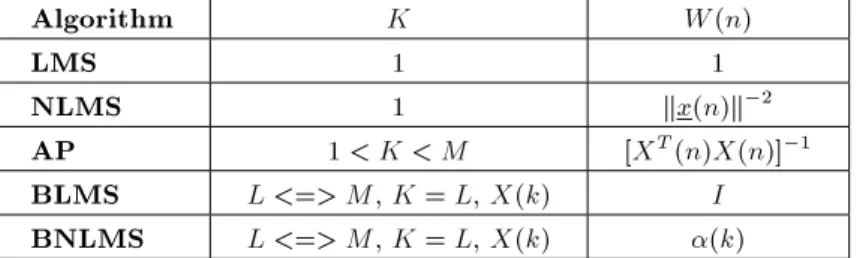
lter algorithms, given by specic choices of K and W (n) corresponding to the LMS, the NLMS and the AP algorithms, can be derived [10]. One can also incorporate the BLMS and BNLMS algorithms in this generic update equation. The particular choices and their corresponding algorithms are summarized as the top ve lines in Table 2. The last two entries in Table 2 will be explained in the following sections. It is interesting to note that the most common adaptive ltering algorithms can be interpreted as some sort of Richardson iteration [12]; the simplest of all iter-ative linear equation solvers, applied to a particular estimated Wiener-Hopf equation.
One now proceeds by determining the optimum step-size, o(n), instead of using in the VSS version of
Equation 1. The latter equation can be stated in terms of weight error vector, "(n) = ht h(n), as follows:
"(n + 1) = "(n) X(n)W (n)e(n): (9) Taking the squared norm and expectations from both sides of Equation 7, one obtains:
Enk"(n + 1)k2o= Enk"(n)k2o
+ 2EeT(n)BT(n)B(n)e(n)
2EeT(n)BT(n)"(n) ; (10)
where B(n) = X(n)W (n). Equation 10 can be represented in the form of Equation 11:
Enk"(n + 1)k2o= Enk"(n)k2o ; (11) where is given by:
= 2EeT(n)BT(n)B(n)e(n)
+ 2EeT(n)BT(n)"(n) : (12)
If is maximized, then, Mean-Square Deviation (MSD) will undergo the largest decrease from iteration n to iteration n + 1. The optimum step-size will be found with a derivation of , with respect to , equal to zero, d
d = 0;
o(n) = E
eT(n)BT(n)"(n)
E feT(n)BT(n)B(n)e(n)g: (13)
Introducing the a priori error vectors:
ea(n) = XT(n)"(n); (14)
it is found, from Equation 7, that the error vector is related to an a priori error vector, via Equation 15:
e(n) = ea(n) + v(n): (15)
Assuming the noise sequence, v(n), is identically and independently distributed and statistically indepen-dent of the regression data, and by neglecting the dependency of "(n) on the past noises, the following two sub equations are established from the two parts of Equation 13:
Part I:
EeT(n)BT(n)"(n)
= E "T(n)X(n) + vT(n) BT(n)"(n)
= E"T(n)X(n)BT(n)"(n) : (16)
Table 2. Correspondence between special cases of Equation 1 and various adaptive ltering algorithms. Algorithm K W (n)
LMS 1 1
NLMS 1 kx(n)k 2
AP 1 < K < M [XT(n)X(n)] 1
BLMS L <=> M, K = L, X(k) I BNLMS L <=> M, K = L, X(k) (k)
Part II:
EeT(n)BT(n)B(n)e(n)
= E"T(n)X(n)BT(n)B(n)XT(n)"(n)
+ EvT(n)BT(n)B(n)v(n)
= E"T(n)X(n)BT(n)B(n)XT(n)"(n)
+ 2 vTr E
BT(n)B(n) : (17)
Finally, by dening C(n) = B(n)XT(n), the optimum
step-size in Equation 13 becomes: o(n) = E
"T(n)CT(n)"(n)
E f"T(n)CT(n)C(n)"(n)g + C; (18)
where: C = 2
vTr E
BT(n)B(n) : (19)
Substituting the o(n) of Equation 18, instead of ,
in Equation 1, the generic variable step-size update equation that covers VSSNLMS and VSSAPA of [6], as special cases, will be obtained. One must now focus on the development of the VSSBNLMS adaptive algorithm.
VARIABLE STEP-SIZE BLOCK
NORMALIZED LMS ADAPTIVE FILTER ALGORITHM
The lter coecients update equation for BNLMS can be stated as:
h(k + 1) = h(k) + X(k)(k)e(k); (20) where k is the block index, h(k) the length, M column vector of lter coecients to be adjusted once after the collection of every block of data samples. X(k) is an M K input signal matrix, d(k) is an K 1 vector of desired signal samples and e(k) is the error signal vector which are dened by:
X(k)=[x(kL); x(kL 1); x(kL 2); ; x(kL K+1)]; (21) d(k)=[d(kL); d(kL 1); d(kL 2); ; d(kL K+1)];
(22) e(k)=[e(kL); e(kL 1); e(kL 2); ; e(kL K+1)];
(23) where L is the block length and the error signal vector is calculated by;
e(k) = d(k) XT(k)h(k): (24)
There are three possible choices for selecting L:
1. L = M, which is the optimal choice from the viewpoint of computational complexity;
2. L < M, which oers the advantage of reduced processing delay. Moreover, by making the block size smaller than the lter length, one still has an adaptive ltering algorithm computationally more ecient than the conventional LMS algorithm; 3. L > M, which gives rise to redundant operations in
the adaptive process, the estimation of the gradient vector (computed over L points) now uses more information that the lter itself.
Selecting L = M is more practical in dierent applica-tions. For the BLMS adaptive lter algorithm (k) = I. In the case of the BNLMS adaptive algorithm, the K K matrix, (k), is a diagonal matrix with the elements, (k) = kX(k)Iik 2, i = 0; 1; K 1,
on the diagonal, where Ii is the column number, i,
of the K K identity matrix, I. Note that terms kX(k)Iik2are the signal power estimates.
Based on the above and by comparing Equa-tion 20 to EquaEqua-tion 1, which in turn, was identied as an iterative solution strategy for Equation 5, it is immediately observed that the BNLMS update can be interpreted as an iterative solution strategy applied to the weighted Wiener-Hopf-type equation, according to the selecting parameters from Table 2. To get a better performance in a BNLMS adaptive lter, the VSSBNLMS adaptive lter algorithm is presented, based on the generic VSS update equation, which was described in the previous section. It is pointed out that this is a block adaptive algorithm, i.e. one lter vector update is performed each time that L new samples have entered the system. It means that the step-size will be updated for every block.
To simplify the formulation 0(k) is dened as a
diagonal matrix with elements 0(k) = kX(k)Iik 1,
i = 0; 1; ; K 1 on the diagonal. Therefore, T 0(k)
is also a diagonal matrix with elements T 0(k) =
kX(k)Iik T, i = 0; 1; ; K 1 on the diagonal. It
is obvious that 0(k) = T0(k).
Also, by introducing the p(k), q(k) and, by using the results from Equation 18;
p(k) = T
0(k)XT(k)"(k); (25)
q(k) = X(k)(k)XT(k)"(k); (26)
the optimum step-size for the BNLMS adaptive lter is given by:
o(k) = E
n
p(k)2o
where C is a positive constant and can be approximated from Equation 19:
C = 2 vTr E
(k)XT(k)X(k)(k) : (28)
In calculating the optimum step-size from Equation 27, the main problem is that p(k) and q(k) are not available, since ht is unknown. Therefore, one needs to estimate these quantities.
By taking expectation from both sides of Equa-tions 25 and 26,
Ep(k) = ET
0(k)XT(k)"(k) ; (29)
Eq(k) = EX(k)(k)XT(k)"(k) ; (30)
and by substituting ea(k) = e(k) v(k) in Equations 29 and 30, one yields:
Ep(k) = ET
0(k)ea(k)
= ET
0(k) (e(k) v(k))
= ET
0(k)e(k) ; (31)
Eq(k) = EX(k)(k)XT(k)"(k)
= E fX(k)(k) (e(k) v(k))g
= E fX(k)(k)e(k)g : (32)
These quantities can be estimated with the recursions, presented in the following equations:
^p(k) = ^p(k 1) + (1 ) T 0(k)e(k)
; (33)
^q(k) = 0^q(k 1) + (1 0) (X(k)(k)e(k)) ; (34)
where and 0are smoothing factors, (0 < , 0< 1).
Finally, the recursion for the variable step-size BNLMS (VSSBNLMS) adaptive algorithm (VSS-BNLMS) is given by:
h(k + 1) = h(k) + (k)X(k)(k)e(k); (35) where:
(k) = max ^p(k) 2
^q(k)2+ C: (36)
The step-size changes with the ^p(k)2, ^q(k)2 and the constant, C, which can be approximated from Equation 28. It is clear that C is inversely proportional to SNR. To guarantee the update stability, max is
selected less than 2.
COMPUTATIONAL COMPLEXITY
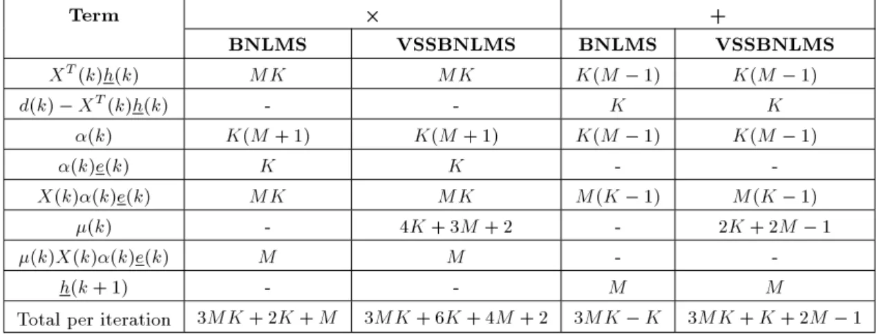
In this section, the computational complexity of the BNLMS and the VSSBNLMS is compared. In Ta-ble 3, the number of real multiplications and real additions that are required in the evaluation of specic terms for both BNLMS and VSSBNLMS adaptive lter algorithms are shown. The only dierence in the computational complexity between BNLMS and VSSBNLMS is in the (k) term. Table 4 shows the number of real multiplications and real additions that are required in the evaluation of this term. The only dierence is 4K + 3M + 2 multiplications and 2K + 2M 1 additions per iteration. It is seen that the cost of BNLMS and VSSBNLMS adaptive lter algorithms is O(MK) operations per iteration. SIMULATION RESULTS
The theoretical results presented in this paper are justied by several computer simulations in a channel estimation setup. The unknown channel has 8 taps
Table 3. Computational cost of BNLMS and VSSBNLMS adaptive lter algorithms per iteration in terms of the number of real multiplications and real additions.
Term +
BNLMS VSSBNLMS BNLMS VSSBNLMS XT(k)h(k) MK MK K(M 1) K(M 1)
d(k) XT(k)h(k) - - K K
(k) K(M + 1) K(M + 1) K(M 1) K(M 1)
(k)e(k) K K -
-X(k)(k)e(k) MK MK M(K 1) M(K 1) (k) - 4K + 3M + 2 - 2K + 2M 1
(k)X(k)(k)e(k) M M -
-h(k + 1) - - M M
Table 4. Computational cost of the step-size in VSSBNLMS per iteration in terms of the number of real multiplications and real additions.
Term +
T
0(k)e(k) K
-(1 )T
0(k)e(k) K
-(1 0)(X(k)(k)e(k)) M
-^p(k) K K
^q(k) M M
^p(k)2 K K 1
^q(k)2 M M 1
(k) 2 1
Total per iteration 4K + 3M + 2 2K + 2M 1
and selected at random. Two dierent types of signal, Gaussian and uniformly distributed signals, are used in forming the input signal, x(n):
x(n) = :x(n 1) + w(n); (37)
which is a rst order autoregressive (AR) process with a pole at . For the Gaussian case, w(n) is a white, zero-mean, Gaussian random sequence, having unit variance, and is set to 0.9. As a result, a highly colored Gaussian signal is generated. For the uniform case, w(n) is a uniformly distributed random sequence between -1.0 and 1.0 and is again set to 0.9. Measurement noise, v(n), with 2
v = 10 3, was added
to the noise-free desired signal generated through d(n) = hT
tx(n). The adaptive lter and the unknown
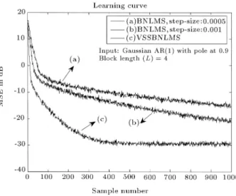
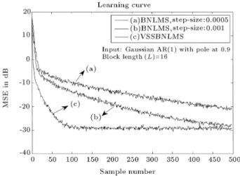
channel are assumed to have the same number of taps. All the simulations are obtained by ensemble averaging over 200 independent trials. Figures 2 to 7 show the learning curves of BNLMS and VSSBNLMS adaptive lter algorithms. Figures 2 to 4 compare the learning curves of BNLMS and VSSBNLMS adaptive algorithms with dierent block length (L = 4; 8; 16) and for highly colored Gaussian input. The ensemble averaged learning curves for VSSBNLMS were obtained with = 0:99, 0= 0:99, C = 0:001 and
max= 1. In
the ordinary BNLMS case, the simulation results were obtained for dierent step-sizes. Figures 5 to 7 show the learning curves for a highly colored uniform input signal. It can clearly be seen that the VSSBNLMS has a fast convergence rate and a low steady-state mean square error, when compared to the ordinary BNLMS algorithm for both highly colored and uniform input signals.
CONCLUSIONS
In this paper, the generic, variable, step-size adaptive lter was presented. This generic VSS adaptive lter can cover VSSNLMS and VSSAPA adaptive lter
Figure 2. Learning curves of BNLMS with various step-sizes and VSSBNLMS adaptive lter algorithms for L = 4. Input: Highly colored Gaussian (Gaussian AR(1) with = 0:9).
Figure 3. Learning curves of BNLMS with various step-sizes and VSSBNLMS adaptive lter algorithms for L = 8. Input: Highly colored Gaussian (Gaussian AR(1) with = 0:9).
Figure 4. Learning curves of BNLMS with various step-sizes and VSSBNLMS adaptive lter algorithms for L = 16. Input: Highly colored Gaussian (Gaussian AR(1) with = 0:9).
Figure 5. Learning curves of BNLMS with various step-sizes and VSSBNLMS adaptive lter algorithms for L = 4. Input: Highly colored uniform (uniform AR(1) with = 0:9).
Figure 6. Learning curves of BNLMS with various step-sizes and VSSBNLMS adaptive lter algorithms for L = 8. Input: Highly colored uniform (uniform AR(1) with = 0:9).
Figure 7. Learning curves of BNLMS with various step-sizes and VSSBNLMS adaptive lter algorithms for L = 16. Input: Highly colored uniform (uniform AR(1) with = 0:9).
algorithms. Following this, the variable step-size BNLMS, named the VSSBNLMS adaptive lter algo-rithm, was developed, based on the generic, variable, step-size adaptive lter. The algorithm exhibits fast convergence, while reducing steady-state mean square error, as compared to the ordinary BNLMS adaptive algorithm.
REFERENCES
1. Haykin, S., Adaptive Filter Theory, NJ, Prentice-Hall, 4th Edition (2002).
2. Sayed, A.H., Fundamentals of Adaptive Filtering, Wi-ley (2003).
3. Pradhan, S.S. and Reddy, V.E. \A new approach to subband adaptive ltering", IEEE Trans. Signal Processing, 47, pp 655-664 (1999).
4. de Courville, M. and Duhamel, P. \Adaptive ltering in subbands using a weighted criterion", IEEE Trans. Signal Processing, 46, pp 2359{2371 (1998).
5. Lee, K.A. and Gan, W.S. \Improving convergence of the NLMS algorithm using constrained subband updates", IEEE Signal Processing Letters, 11, pp 736-739 (2004).
6. Shin, H.C., Sayed, A.H. and Song, W.J. \Variable step-size NLMS and ane projection algorithms", IEEE Signal Processing Letters, 11, pp 132-135 (Feb. 2004). 7. Husy, J.H. and Abadi, M.S.E. \A common framework for transient analysis of adaptive lters", in Proc. Melecon, Dubrovnik, Croatia, pp 265-268 (May 2004). 8. Husy, J.H. \On performance analysis of transform domain adaptive lters: A unied perspective", in 15th Intl. Czech-Slovac Sci. Conf. Radioelecktronika, Brno, Czec Republic, pp 96-99 (May 2005).
9. Husy, J.H. \A novel interpretation and performance analysis of subband adaptive lter algorithms", in
Proc. of Seventh Intl. Symp. on Signals. Circuits and Systems, 2, pp 561-564, Iasi, Romania (2005). 10. Husy, J.H. \A unied framework for adaptive
lter-ing", in Proc. NORSIG, Bergen, Norway, CD-ROM, ISBN 82-993158-5-9 (Oct. 2003)
11. Husy, J.H. \Adaptive lters viewed as iterative linear equation solvers", in Ser. Lecture Notes in Computer Science, Springer-Verlag, 3401, pp 320-327 (2005).
12. Husy, J.H. and Abadi, M.S.E. \Transient analysis of adaptive lters using a general framework", in AUTOMATIKA, Journal for Control, Measurement, Electronics, Computing and Communications, 3-4/45, pp 121-127 (2004).
13. Saad, Y., Iterative Methods for Sparse Linear Systems, PWS Publishing (1996).