for Multivariate Risks
by Maochao Xu
ABSTRACT
This paper studies a novel capital allocation framework based
on the tail mean-variance (TMV) principle for multivariate risks.
The new capital allocation model has many intriguing
proper-ties, such as controlling the magnitude and variability of tail
risks simultaneously. General formulas for optimal capital
allo-cations are discussed according to the semideviation distance
measure. In particular, we discuss the optimal capital allocation
for comonotonic risks, and risks from multivariate elliptical
dis-tribution and multivariate skew-t disdis-tribution. Some numerical
examples are given to illustrate the results, and real data from an
insurance company is analyzed as well.
KEYWORDS
Recently, Dhaene et al. (2012) proposed a criterion to set the capital amountki toXi as close as possible to minimize the loss. Specifically, the criterion is to minimize the following loss function
L D Xi ki
i n
∑
(
)
( ) −
=
k = , (1.1)
1
whereD is some suitable distance measurement func-tion, andk=(k1, . . . ,kn)∈Rn. A lot of work has been motivated by this criterion; see Xu and Hu (2012), Zaks (2013), Cheung, Rong, and Yam (2014), and others. In fact, the idea of minimizing the loss func-tion has been discussed in the framework of premium calculation. For example, Zaks et al. (2006) used quadratic distance measure D(x) = x2, and Laeven and Goovaerts (2004) used the semi-deviation func-tionD(x)= max{x, 0} as distance measure. This topic was further pursued in Frostig, Zaks and Levikson (2007), where they used the general convex distance measure. However, most of the discussion on capi-tal allocations in the literature has focused only on the magnitude of the loss functionL. In practice, the variability also plays an essential role in determin-ing the capital allocations. Indeed, the relevant idea has already appeared in the premium calculation. Furman and Landsman (2006) used the tail variance risk measure to estimate the variability along the tails, and to compute the premium based on the tail vari-ance premium (TVP) model
TVPq( )X =TCEq( )X + βTVq( )X , β ≥0,
where TCEqand TVqrepresent tail conditional expecta-tion, and tail conditional variance, respectively. That is,
E
X X X x
V X X X x
q q
q q
(
)
(
)
( ) ( )
= >
= >
TCE ,
T Var ,
wherexq isqth quantile of riskX. See also Landsman, Pat, and Dhaene (2013) for the discussion on the tail variance related premium calculation. Motivated by this observation, Xu and Mao (2013) proposed a TMV model to discuss the optimal capital alloca-tions, where they defined the loss function as
1. Introduction and motivation
In the actuarial literature, a fundamental question is how to allocate the total amount of risk capital to different subportfolios, divisions, or lines of busi-nesses. The allocation problem is very important since the amount of risk capital allocated to a busi-ness consisting of multiple lines of busibusi-nesses is typically less than the sum of amounts of risk capi-tal that would need to be withheld for each business separately. Heterogeneity and dependence that may exist between the performances of various business units make capital allocation a nontrivial exercise. Therefore, there exists an extensive amount of liter-ature on this subject with a number of proposed cap-ital allocation algorithms. For example, Myers and Read (2001) considered capital allocation principles based on the marginal contribution of each business unit to the company’s default option. Denault (2001) discussed capital allocations from the perspective of game theory. The first multivariate top-down model considered in Panjer (2002) studies the particu-lar case of multivariate, normally distributed risks and provides an explicit expression of marginal cost-based allocations using TVaR (tail value-at-risk) risk measure. This work has been extended by Landsman and Valdez (2003) to model risks using multivariate elliptical distributions, which include the multivariate normal as a special case; see also Dhaene et al. (2008). Furman and Landsman (2005) studied the capital allocation for the risks follow-ing multivariate gamma distributions. Cossette et al. (2013) discussed the multivariate risks with mixed Erlang marginals and the dependence structure is modeled by the Farlie-Gumbel-Morgenstern copula. One may refer to Dhaene et al. (2012), Xu and Hu (2012), Tsanakas (2004), and Furman and Zitikis (2008) and references therein for the recent devel-opments on this topic.
Assume that a firm has a portfolio of risksX1, . . . ,Xn, and wishes to allocate the total capitalK=k1+ . . .+k
n to the corresponding risks. The total risk is then
Initiative) each year. For example, DHS allocated a total of $490.4 million in 2012, $558.7 million in 2013, and $587.0 million in 2014 to urban areas to prevent terrorist attacks.1The effective alloca-tion of the total capital to urban areas is an impor-tant but challenging problem, which has received much attention in the security area (cf. Hu, Homem-de-Mello, and Mehrotra 2011). A popular distance measure used in this area is the semideviation func-tion. In fact, in the literature of actuary science, the semideviation function has been widely used in the stop-loss premium calculation (Dhaene et al. 2012). Based on the above discussion, in this paper, we are motivated to study the capital allocation based on the TMV model with the loss function defined as
X k
L q Xi ki S q S
i n
∑
[
]
(
)
= ( − )+ > ( )=
; , VaR .
1
We consider the following general mean-variance model,
R
X
∑
{
}
[
(
)
]
π
= ∈ = =
∈
min ; , ;
. . : , 1, . . . , .
(1.2)
=1
k k
k A L q
s t A n k K i n
i i n
wherep(.) is the mean-variance risk measurement,
andb ≥ 0. It is worth pointing out that Laeven and Goovaerts (2004) considered a special case of the
TMV model (1.2). They discussed the case ofn = 2
but without considering the tail risks. Specifically, they discussed the optimal capital allocation based on mini-mizing the following loss function,
X;
Var ,
1 1 2 2
1 1 2 2
E k
L X k X k
X k X k
[
]
[
]
[
(
)
]
(
)
( )( ) ( )
π = − + −
+ β − + −
+ +
+ +
overk∈A. Therefore, the TMV model (1.2) is a natural extension of their model.
Our main contributions in this paper are summa-rized as follows. First, we derive the general equations
k
X
G q Xi ki S q S
i n
; , 2 VaR ,
1
∑
[
]
(
)
= ( − ) > ( )=
where VaRq(S) is theqth quantile of S, and consid-ered the following function
X; ,k E X; ,k Var X; ,k ,
G q G q G q
[
(
)
]
[
(
)
]
(
(
)
)
π = + β
where p(.) is the mean-variance risk measurement, which has been widely used in practice (Laeven and Goovaerts 2004). The TMV model has many intrigu-ing properties, such as simultaneously controllintrigu-ing the magnitude and variability of tail loss, and pro-viding neat optimal allocation formulas. From the economic perspective, the perfect case is that the company could prepare the capital to match the loss exactly, since too much or less capital would result in the loss of revenue for a company. Therefore, a com-pany should prefer a capital allocation rule which could provide the capital to match the loss as close as possible. It is apparent that controlling the magnitude of deviation of the capital from the loss is important. However, the variability of deviation is also essen-tial in determining the required capital, as the larger variability would lead to more risk for the company. Therefore, the property of controlling the magni-tude and variability is appealing in determining the required capital for business lines.
In practice, however, the shortage of capital may often result in much severer consequences than that caused by the excess of capital (Myers and Read 2001; Erel, Myers and Read 2013), which suggests that the semideviation function may be preferred in practice as the distance measure. This issue is also related to the capital allocation of homeland secu-rity, an area that has become centrally important since the terrorist attacks of September 11, 2001. Since catastrophes are highly risky and could lead to severe consequences, the Department of Homeland Security (DHS) has endeavored to use risk manage-ment to determine the capital allocations on pre-vention, response, and recovery from such national catastrophes. The budget in DHS is allocated via the program called UASI (Urban Area Security
1The data is from the website of Federal Emergency ManagementAgency,
In the following, by using the methodology of Lagrange multipliers, we present the optimal capital allocation equations based on the TMV model (1.2), and the uniqueness condition is also given. The proof is moved to the Appendix for the sake of readability.
Theorem 2.1.For the TMV model (1.2), assume thatX1, . . . ,Xn are continuous risks, then an optimal allocation solutionk*= (k1*, . . . ,kn*) is given by the following equations, for anyl= 1, 2, . . . ,n,
2 Cov ,
* * *
2 Cov , (2.1)
* * *
.
=1 ,
1. 1
=1
, 1
F k k k
F k k k
l S l j
n
S j l
S
j n
S j
∑
∑
( )
(
)
( )
(
)
+ β
= + β
+
+
and
k* . . .1 + +k*n=K.
Further, if, for anyl= 1, 2, . . . ,n,
1 2 * *, VaR
2 ECT * (2.2)
=1
E X k X k S S
k
j j l l q
j l n
S j
n
j
∑
∑
(
)
( )
( )+ β − = >
> β
+ ≠
then the solution is unique.
From Theorem 2.1, it is seen that the capital allo-cations based on Model (1.2) depend not only on the magnitude of tail risks but also the covariance among the tail risks. This property would allow the com-pany to control the tail risks from both the magnitude and variability perspectives. In general, there does not exist an analytical solution to Eq. (2.1). The key quantities required to solve the equation are F–i.S(.), ECTS(.), and Cov+,S(., .), which, however, could be efficiently computed by using any computer soft-ware; see Section 4 for examples. It can be seen from Eq. (2.2) that when b is small, then the uniqueness condition is easily satisfied. In the following, we dis-cuss a special case ofb = 0 for Theorem 2.1, i.e., with-out considering the penalty on the tail variance. For this case, a closed-form solution could be obtained. for the TMV model (1.2), based on which the
numer-ical programming could be easily implemented. Second, we discuss the special case of comonotonic risks, and the closed-form solutions are obtained. Third, we compute the key quantities of optimal capital allocation formulas for multivariate elliptical distributions, and Monte Carlo simulation for those quantities of multivariate skew-t distributions is also mentioned. Finally, we conduct a real data analysis and discuss the optimal capital allocation based on the new model.
The rest of the paper is organized as follows. In Section 2, we derive the general equations for the TMV model, and discuss a special case. Section 3 studies the optimal capital allocations for the como-notonic risks. In Section 4, we present some numeri-cal examples to illustrate the different factors that affect the capital allocations and conduct a real data analysis of capital allocations for an insurance com-pany. In the last section, we summarize the results and present some discussion.
2. Optimal capital allocation:
General results
In this section, we provide general capital alloca-tion equaalloca-tions for the TMV model (1.2). To facilitate the discussion, let us denote the conditional survival function of [XiS> VaRq(S)] by
Fi S. ( )ki =P
(
Xi >k Si >VaRq( )S)
, i=1, . . . , .nThe conditional expectation of risk excess [(Xi –ki)+
S> VaRq(S)] is denoted by
k X k S S
S i i i q
ECT ( )=E
[
(
−)
+ >VaR ( )]
,and the covariance between [(Xi –ki)+S > VaRq(S)] and [I(Xj≥kj)S> VaRq(S)] is represented by
Cov ,
Cov , I > VaR ,
, k k
X k X k S S
S i j
i i j j q
[
]
(
)
(
)
(
)
( )= − ≥
+
+
3. Comonotonic risks
Comonotonicity, an extremal form of positive dependence, has been widely used in finance and actuarial science over the last two decades. It is well known that the comonotonic random variables are always moving in the same direction simultane-ously and hence are considered as extreme depen-dent risks. Refer to Dhaene et al. (2002a; 2002b) for the properties and applications of this concept in actuarial science and finance. For a company with several business lines, it is particularly impor-tant for them to prepare for the worst scenario. It is known in the literature that the aggregate risk of comonotonic risks with finite means may be regarded as the most dangerous case in terms of convex order (Dhaene et al. 2002a). From the per-spective of capital allocation allocations, it would be interesting to know whether the comonotonic dependence structure among risks is the most dan-gerous case in terms of some stochastic measure. Further, if it is the most dangerous scenario, what is the optimal capital allocation strategy? In this sec-tion, we first show that the comonotonic risks are the most dangerous risks for the capital allocations in the sense that the expected tail loss is the larg-est. Then, we discuss the optimal capital allocation based on the TMV model (1.2). We need the follow-ing two lemmas.
The first lemma presents an equivalent charac-terization of a comonotonic random vector (Dhaene et al. 2002a).
Lemma 3.1.A random vector (X1, . . . ,Xn) is como-notonic if and only if there are increasing real-valued functionsf1, . . . ,fn and and a random variableW such that
, . . . , , . . . , ,
1 1
(X Xn)=st(f W( ) f Wn( ))
where =st represents that both sides of equality have the same distribution.
The following lemma, essentially due to Sordo et al. (2013), will also be used in the sequel.
Corollary 2.2. Under the same condition of Theo-rem 2.1, forb = 0, a unique optimal allocation solu-tionk*= (k1*, . . . ,kn*) is given by
k*i =Fi S−.1
(
FSc( )K)
, i=1, . . . , ,nwhere
,
.1 1
∑
( )= −
=
Sc F U
i S i
n
withF–1
i.S(U)= [XiS> VaRq(S)] almost surely.
Proof: According to Theorem 2.1, the optimal solution should satisfy the following equations:
* * (2.3)
. 1. 1
Fl S
( )
kl =FS( )
kforl= 2, . . . ,n andk1*+ . . .+kn*=K. Now define the
,
.1 1
∑
( )= −
=
Sc F U
i S i
n
whereU is the uniform random variable on [0, 1]. It is known from Dhaene et al. (2012) that there exists some 0≤ a ≤ 1 such that
Fi S FS K K
i n
c
∑
− α( )(
( ) =)
=,
.1 1
where Fi.S–1(a)(.) is the a-mixed inverse distribution function. Therefore, an optimal solution is given by
*= .− α1( )
(
( ))
, =1, . . . , ,ki Fi S FSc K i n
which satisfies Eq. (2.3). Moreover, the uniqueness condition in Eq. (2.2) is fulfilled sinceb = 0.
Hence, the required result follows.
Theorem 3.4. Under Model (1.2), a unique optimal allocation solutionk*= (k1*, . . . ,kn*) when (X1, . . . ,Xn) are comonotonic risks with strictly increasing distri-butions is given by
k*i =Fi S−.1
(
FSc( )K)
, i=1 , . . . , ,n (3.1)where S--c =
Σ
ni=1 F–1i.S(U), with Fi.S–1(U) = [XiS > VaRq(S)] almost surely.
Proof: Note that
Cov * *,
Cov * , I * VaR
Cov * , I * VaR .
, 1
1
1
k k
X k X k S S
X k X k S S
S j n j l j n
j j l l q
j j
j n
l l q
∑
∑
∑
[
]
(
)
(
)
(
)
(
)
(
)
( ) ( )= − ≥ >
= − ≥ >
+ = = + + =
Since (X1, . . . ,Xn) is a comonotonic vector, it holds that
, . . . , VaR
1
[
(X X Sn) > q( )S]
is also comonotonic, and, further,
, . . . , VaR
* *
1 1
X k Xn kn S q S
[
(
−)
+(
−)
+ > ( )]
is comonotonic. According to Proposition 1 of Cheung (2009), it holds that
VaR *
VaR ,
1 . .
X k S S
S K S S
i i q
i n a s q
∑
(
)
[
]
( ) ( ) ( ) − > = − >
+ =
+
wherea.s.=
represents both sides are almost surely equal. Therefore, we have
X k X k S S
S K X k S S
S K
F X F K S S
S K U F K S S
j j l l q
j n
l l q
l S l S q
S q c c
∑
[
]
(
)
(
)
(
)
]
]
[
[
(
)
(
)
( ) ( ) ( ) ( ) ( ) ( ) ( ) ( ) ( ) ( )− ≥ >
= − ≥ >
= −
≥ >
= − ≥ >
+ =
+
+
+
Cov * , I * VaR
Cov , I * VaR
Cov ,
I VaR
Cov , I VaR .
1
.
Lemma 3.2. LetX andY be two continuous risks with strictly increasing distribution functionsF andG, respectively. Then, forq∈(0, 1], it holds that
X Y G q st X X F q
[
> −1( )] [
≤ > −1( )]
,where≤st represents the usual stochastic order (Shaked and Shanthikumar 2007). Particularly ifX and Y are comonotonic, then
X Y G q st X X F q
[
> −1( )] [
= > −1( )]
.By utilizing the above two lemmas, we show that the comonotonic risks result in the largest tail losses, which may have its own interest.
Theorem 3.3. Let (X1, . . . , Xn) be a continuous random vector with strictly increasing distribution functions, and (Xc
1, . . . ,Xcn) represents its comono-tonic counterpart. Then,
E
E
∑
∑
(
)
( )
( )
( − ) >
≤ − >
+ =
+ =
X k S S
X k S S
i i q
i n
ic i c q c
i n VaR VaR . 1 1
Proof: Since (Xc
i, Sc) are comonotonic for i = 1, . . . ,n, from Lemma 3.1 it follows that
,
Xic ki Sc
(
(
−)
+)
are also comonotonic, since h(x) = (x – ki)+ is an
increasing function of x. Therefore, according to
Lemma 3.2, we have
X k S S
X k X k X k
X k X k X k
X k S S
ic i c q c
st
ic i ic i q ic i
st
i i i i q i i
st i i q
[
]
[
]
[
]
(
)
(
)
(
) (
)
(
)
[
]
( ) ( ) ( ) ( ) ( ) ( ) ( ) − >= − − > −
= − − > −
≥ − >
+ + + + + + + + VaR VaR VaR VaR .
Hence, the required result follows immediately.
Now, let us discuss the optimal capital allocation based on Model (1.2) for this worst scenario, i.e.,
It includes many well-known distributions, such as multivariate normal distribution, multivariate t distribution, multivariate logistic distribution, and multivariate exponential power distribution, etc. For more discussion of elliptical distribution, one may refer to Fang, Kotz, and Ng (1987) and Landsman and Valdez (2003).
In the following, we first give a brief review of some properties of elliptical distribution, which is pertinent to the discussion of our main results.
Definition 4.1.The random vectorXhas a multi-variate elliptical distribution, denoted byX∼En(m,Σ,
y), if its characteristic function can be expressed as
t t t t
X( ) exp
(
i T) (
T 2)
φ = µ ψ Σ
for some column-vector m, n × n positive definite matrixΣ, and characteristic generatory(.).
It should be pointed out that not every multivari-ate elliptical distribution has a density function. If
X∼En(m,Σ,y), andX has a densityfX(x), then,
x x x
X
1
2 , (4.1)
1 2
1
f cn g
n T
( )= ( ) ( )
Σ − µ Σ− − µ
where
2
2 2 ,
2 1 0
1
cn nn x g x dx
n n
∫
(
)
( )
( ) ( )
= Γ
π −
∞ −
and
,
2 1 0
∫
∞xn − g x dx( ) < ∞n
which guarantees gn(x) to be the density generator. For this case, one may writeX∼En(m,Σ,gn).
If the mean exists, we haveE(X) = m. The condi-tion guarantees the existence of the covariance matrix
y′(0)< ∞ and hence
X
Cov( ) = − ′ψ ( )0 .Σ
Without loss of generality, in the following discussion, it is assumed that –y′(0)= 1, and hence Cov(X)= Σ. For the comprehensive discussion of properties of It is seen that Eq. (2.1) is fulfilled ifk* is a
solu-tion. We conclude thatk* is an optimal solution for Model (1.2). Further, the solution k* is unique, as
it does not depend on the parameterb. Hence, the
required result follows.
Theorem 3.4 presents a closed-form solution of capital allocations for the comonotonic risks. It might be a little surprising to observe that the optimal capital allocation rule based on Model (1.2) for comonotonic risks adopts the same formulas as that in Corollary 2.2, i.e., without the penalty on the tail variance. A care-ful checking of Theorem 2.1 reveals that, although the formulas are the same, the meanings are quite dif-ferent for both scenarios. Corollary 2.2 presents the optimal capital allocations for any dependence struc-ture by considering only the magnitude of tail risks. However, Theorem 3.4 presents the optimal capital allocations for the comonotonic risks by considering both the magnitude and variability of tail risks. But, for this particular dependence structure, the magni-tude and variability of loss functions are minimized simultaneously, which explains the same optimal capital allocation formulas as in Corollary 2.2. One may wonder whether the magnitude and variability of loss functions could be minimized simultaneously for other general multivariate risks, i.e.,b is irrelevant to the optimal capital allocations. The answer is negative from the examples in Section 4. In fact, the penalty parameterb has nonnegligible influence on the capi-tal allocations.
4. Examples and applications
In this section, we present some examples of opti-mal capital allocations based on Model (1.2) for spe-cific multivariate distributions. We will also apply the new capital allocation rule to real data from one insurance company.
4.1. Elliptical distributions
2 2 1 1 1 2 2
1 2 2 , (4.3)
1 . VaR 1 . 2 . 1 , 1 2 , 1 2 . , 1 VaR . 2 . 1 2 , 1 2 1 2 * 1 2 * c g x c g s qdsdx c q
g x g s dsdx
c
q g
z
dz g w dw
ii S S k i s ii S S S S S S
ii S S S
S k i s ii S S S S z w q i q i
∫
∫
∫
∫
∫
∫
( ) ( ) ( ) ( ) ( ) = σ − µ σ σ − µ σ − =σ σ −
−µ σ
− µσ
= − ( ) ( ) ∞ ∞ ∞ ∞ ∞ ∞
wherez* = (ki – mi.w′)/ σii S. withw′ = σii S. w+ mS, andw*= (VaRq(S) –mS)/ σSS. The notationfi(.S> VaRq(S)) represents the density function of [XiS >
VaRq(S)]. and FS(sS > VaRq(S)) represents the dis-tribution function of [SS> VaRq(S)].
Next, we provide a simple form for computing ECTS(.).
ECT VaR VaR 2 2 1 1 1 2 2 (4.4) 1 . 1 Var . 2 . 1 , 1 2 , 1 2 . . 1 2 * * 1 2 E
k X k S S
x k f x S S dx
x k c g x
c g s qdsdx c q z k g z dz
g w dw
S i i i q
i
k i q
i ii S S k i s ii S S S S S S ii S
i w i z w i q i
∫
∫
∫
∫
∫
[
]
(
)
( ) ( ) ( ) ( ) ( ) ( ) ( ) ( )= − >
= − >
= − σ − µ σ σ − µ σ − = − σ + µ − ( ) + ∞ ∞ ∞ ′ ∞ ∞
The conditional covariance Cov+,S(ki,kj) can be rep-resented as
Cov , I VaR
ECT .
,
.
E
k k X k X k S S
k F k
S i j i i j j q
S i j S j
[
]
(
)
(
)
( )
( ) ( ) ( )= − ≥ >
−
+ +
Note that
I VaR
, VaR ,
(4.5)
,
E X k X k S S
x k f x x S S dx dx
i i j j q
i i i j i j q i j
k ki
∫
j∫
[
]
(
)
(
)
( ) ( ) ( ) ( )− ≥ >
= − >
+ ∞ ∞
elliptical distributions, please refer to Fang, Kotz, and Ng (1987).
We first recall the well-known property of elliptical distributions.
Proposition 4.2. IfX∼En(m,Σ,gn), andA is some
m×n matrix of rankm≤n, andb somem-dimensional column-vector, then
X b∼ b, , .
A + E Am
(
µ + A A gΣ T m)
Next, we compute the key quantities, including
F–i.S(.), ECTS(.), and Cov+,S(., .) for the family of elliptical distributions, which would facilitate the computations of Eq. (2.1).
Note that if X ∼ En(m, Σ, gn), then by Proposi-tion 4.2, it holds that
∼ 1 , , , 1 ,
S E (µ σS S S g )
where mS = Σni=1mi, and sS,S = Σnj=1Σni=1sij with sij = Cov(Xi,Xj). Further, by Xu and Mao (2013), we have
∼
, 2 . , . , 2 , (4.2)
X X Si j s E ij s ij S g
(
=)
(
µ Σ)
where , . . . , , , , , , , , s s ij s i s j s
i S S S i S i S S S
j S S S j S j S S S
(
)
( )
µ =µµ = σ σ + µ − µ σ σ σ σ + µ − µ σ σ and . . . . . . , 2 , , , ,
, , , 2, ,
ij S
ii S ij S
ji S jj S
ii i S S S ij i S j S S S
ji i S j S S S jj j S S S
Σ = σ σ
σ σ
= σ − σ σ σ − σ σ σ σ − σ σ σ σ − σ σ
withsi,S= Σnk=1sik.
The survival function of [XiS> VaRq(S)] can be computed as VaR VaR . VaR
∫
∫
∫
(
)
(
)
( ) ( ) ( )( ) = >
= ( ) = >
∞
∞ ∞
F k f x S S dx
f x S s dF s S S dx
i S i k i q
i S
k S q
dependence, variance penalty parameter b, risk level q, and heavy tail. Assume that an insurance company has three business lines (X1,X2,X3), which follow the multivariate student t distribution with mean vector
6,10, 5 ,
( )
µ =
and
1 3
1 .
12 13
21 23
31 32
Σ =
σ σ
σ σ
σ σ
The total capital is assumed to beK= 25. In the fol-lowing, we examine several scenarios by varying the parameterss12,s13 ands23. The results are summa-rized in Table 1, which are thoroughly discussed as follows.
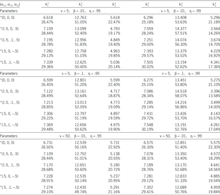
• Dependence effect. To study the dependence effect, we vary the values ofs12,s13ands23. As seen from Table 1, whens12 ranges from {0, .5, 1.5} ands23 from {–.5, 0, .5}, the more dependence results the more capital requirement. For example, for the case (n,b, q) = (5, .01, .95), whens12 changes from 0 to .5, ands23 changes from 0 to –.5, it is found that the required capital for riskX1 increases from 6.618 (26.47%) to 7.280 (29.12%), but risk X3 reduces
from 5.618 (22.47%) to 4.963 (19.85%); whens13
changes from 0 to .1, which indicates increasing the dependence betweenX1 andX3, it is found out that the capital requirement forX3 increases from 4.793 (19.17%) to 4.849 (19.40%).
• Penaltyb. From Table 1, it is observed that whenb
changes from .01 to .1, the capital requirement on
X2 increases for all the cases. This is very reason-able since X2 is the riskiest one. For example, for (s12,s13,s23)=(1.5, .1, .5) and (n,q)=(5.99), when b changes from .01 to .1, the allocation amount changes from 14.074 (56.30%) to 14.216 (56.86%), which reflects the penalty on the variance of new model as expected.
• Risk levelq. Table 1 presents the capital alloca-tions for two risk levelsq= .95 andq=.99. The where fi,j(., .S > Varq(S)) is the joint density
func-tion of [(Xi,Xj)S > VaRq(S)], which has the follow-ing form
, VaR
, VaR
1
1 ,
2 ,
,
, VaR
1 ,
, VaR
1
2
,
f x x S S
f x x S s dF s S S
q c
f x x S s
g s ds
i j i j q
i j i j
S S q
S S
i j i j S
S
S S
q
q
∫
∫
(
)
(
)
(
)
(
)
( )
( )
( )
>
= = >
=
− σ =
− µ σ
( )
( ) ∞
∞
where fi,j(xi, xjS = s) is the density function of [(Xi,Xj)S=s], which is the bivariate elliptical dis-tribution by Eq. (4.2). One may easily implement the forms of Eqs. (4.3), (4.4) and (4.5) into Eq. (2.1) to derive the solutions.
In the following, we present a numerical example to study the optimal capital allocations based on Model (1.2).
Example 4.3. An n-dimensional multivariate student-t distribution belongs to an elliptical family if its density generator can be expressed as
( ) = +
−
g x x
k n
p p
1
where p > n/2, and kp is some constant depending onp. For simplicity, we assume thatp=n+ n with the degree of freedomn, andkp= n/2. The joint den-sity has the following form:
x 1 x x , (4.6)
1 2
f cn T
n
( )= ( ) ( )
Σ +
− µ Σ − µ ν
( )
− − +ν
where
2
2 .
2
cn ( n ) n
( )
( ) ( )
= Γ + ν
Γ ν πν −
• Tail effect. The cases of n = 5 and n = 50 are used to calculate the capital allocations in Table 1, which represent different tail thickness of marginal distributions. It is known that when
n is smaller, the tail probability of t distribution is larger. It is clearly seen from Table 1 that when
n is smaller, the capital allocation requirement is larger. For example, it is seen that when (s12,s13,
s23)= (.5, .1, –.5), the capital requirement ofX2 is 12.625 (50.40%) based on (n,b,q)=(5, .01, .95) compared to that of 12.435 (49.74%) based on (n,b,q)= (50, .01, .95).
risk level increases, reflecting that the insurance company is more conservative about the risk. Hence the insurance company may be willing to allocate the more capital to the business lines with larger risks. It is seen from Table 1 that the capital allocation to X2 increases for all cases, which meets the aim of controlling the risk. For example, it is seen that when (s12,s13,s23)= (1.5, .1, .5), for the case of (n,b)= (5, .1), the capital requirement of X2 is 14.216 (56.86%) based on
q = .99 compared to that of 13.013 (52.05%)
based onq= .95.
Table 1. Optimal capital allocations (amounts and percentages) based on the TMV model (1.2) with a total capitalK 25.
(s12,s13,s23) k1* k*2 k*3 k*1 k*2 k*3
Parameters v= 5, b = .01, q= .95 v= 5, b = .01, q= .99
*(0, 0, 0) 6.618
26.47% 12.76351.05% 22.47%5.618 25.18%6.296 13.40853.63% 21.18%5.296
*(1.5, 0, .5) 7.109
28.44% 13.09952.40% 19.17%4.793 28.24%7.059 14.37757.51% 14.26%3.564
*(1.5, .1, .5) 7.195
28.78% 12.95651.83% 19.40%4.849 29.00%7.251 14.07456.30% 14.70%3.674
*(.5, 0, –.5) 7.280
29.12% 12.75851.03% 19.85%4.963 29.57%7.393 13.37953.52% 16.92%4.229
*(.5, .1, –.5) 7.339
29.36% 12.62550.40% 20.14%5.036 30.02%7.505 13.15452.62% 17.36%4.341
Parameters v= 5, b = .1, q= .95 v= 5, b = .1, q= .99
*(0, 0, 0) 6.599
26.40% 12.80151.20% 22.40%5.599 25.10%6.275 13.45153.80% 21.10%5.275
*(1.5, 0, .5) 7.122
28.49% 13.16152.64% 18.87%4.717 28.34%7.086 14.51858.07% 13.58%3.396
*(1.5, .1, .5) 7.213
28.85% 13.01352.05% 19.09%4.773 29.14%7.285 14.21656.86% 14.00%3.499
*(.5, 0, –.5) 7.306
29.22% 12.79751.19% 19.59%4.897 29.72%7.431 13.42653.70% 16.57%4.143
*(.5,.1, –.5) 7.369
29.48% 12.65650.62% 19.90%4.975 30.19%7.548 13.19152.76% 17.04%4.261
Parameters v= 50, b = .01, q= .95 v= 50, b = .01, q= .99
*(0, 0, 0) 6.731
26.92% 12.53950.16% 22.92%5.731 26.30%6.575 12.85151.40% 22.30%5.575
*(1.5, 0, .5) 7.109
28.44% 12.75251.01% 20.55%5.138 28.31%7.078 13.35053.40% 18.29%4.572
*(1.5, .1, .5) 7.170
28.68% 12.65150.60% 20.72%5.180 28.76%7.189 13.17052.68% 18.56%4.641
*(.5, 0, –.5) 7.228
28.91% 12.53550.14% 20.95%5.237 29.12%7.281 12.83351.33% 19.54%4.885
*(.5, .1, –.5) 7.274
represents the density function of usualn-dimensional Student’s t distribution with location ξ, positive definite n × n dispersion matrix W, and T1(.;n) denotes the univariate standard Student’st cumula-tive distribution function with degrees of freedom
n > 0.
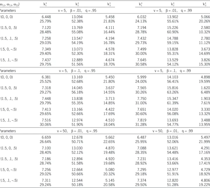
It should be mentioned that although the multi-variate skew-t distribution has many similar proper-ties to the multivariate t distribution, it does not have the preservation property that the conditional distri-bution is still in the original family of distridistri-butions. Therefore, the analytical forms of the key quanti-ties in Eq. (2.1) are infeasible to derive. Instead, we propose to use the Monte Carlo simulation method to compute the key quantities. Specifically, we gen-erate 1,000,000 observations from the multivariate skew-t distribution to computeF–i,S(.), ECTS(.), and Cov+,S(., .), which are illustrated by the following spe-cific example.
Example 4.5.Assume that an insurance company has three business lines (X1,X2, X3), which follow the multivariate skew-t distribution with location parameters
6,10, 5 ,
( )
ξ =
and shape parameters
10, 30, 20 .
( )
α =
The dispersion matrix is assumed to be
1 3
1 .
12 13
21 23
31 32
Ω =
ω ω
ω ω
ω ω
We note that although the dispersion matrix is not the covariance matrix, it is linearly related to the cova-riance matrix, which still reflects the dependence between (X1,X2,X3). The specific relation may be found in Eq. (6.26) of Azzalini (2014).
We use the same parameters as that in Table 1 to compute the optimal capital allocations based on Eq. (2.1). The results are summarized in Table 2. From this example, it is observed that Model (1.2)
has many intriguing properties, such as reflecting the effects of dependence, penalty, tail, and risk level. The numerical results also possess the intuitive expla-nations. It should be pointed out that the elliptical distributions discussed here are symmetric. In the fol-lowing section, we discuss a family of skewed multi-variate distributions.
4.2. Multivariate skew-t family
Insurance risks may have skewed distributions, for which the symmetric distributions such as multi-variate normal or t distributions are not appropri-ate models for insurance risks or losses. Therefore, in the literature, the multivariate skewed distribu-tions have been proposed as alternatives to model such risks. Among many multivariate skewed distributions, the multivariate skew-t distribution has been favored since it provides the benefit of flexibility with regard to skewness and thickness of the tails. It allows unlimited range for the indices of skewness and kurtosis for the individual com-ponents. For a comprehensive discussion about skewed-distribution family, one may refer to Azzalini (2014).
In the following, we give the definition of a multi-variate skew-t distribution.
Definition 4.4.The random vector X has a multi-variate skew-t distribution, denoted byX∼ST(ξ,W,
a,n), if its density function can be expressed as
x x
x
x
X 2 ; , ,
;
1 1
1 2
f t
T w p
Q n
n
T
(
)
(
)
( )
( )
= ξ Ω ν
α − ξ ν +
ν +
ν +
−
whereQ(x)= (x –ξ)TW–1(x –ξ),a ∈Rn is the shape parameter, and
x
x
; , , 2
2 1
1 2 2
2
t n
Q
n n
n
(
)
( )( )
( )
( ) ( ) ξ Ω ν = Γ ν +
Ω νπ Γ ν
+ ν
4.3. Comparisons to other methods
In this section, we compare the TMV model (1.2) to several models frequently used in the literature. For comprehensive reviews on the methodologies of capi-tal allocations, one may refer to Dhaene et al. (2012), and Bauer and Zanjani (2013). Specifically, the capital allocation rules considered in this section include:(a) Haircut allocation:
1 1 1
∑
( )( ) = − −=
k F q
F q K
i X
X j n i
j
For the multivariate skew-t distributions, we may draw similar conclusions to those in Example 4.3, i.e., the dependence, penalty parameter b, risk level, and tail thickness all have significant effects on the capital allocations based on Model (1.2). It is interesting to observe that the capital require-ments on risk X2 in Table 2 are larger than the corresponding ones in Table 1. This may be intui-tively explained by the large skewness of risk X2. Hence, in practice, one should always seek a suit-ably skewed distribution if the faced risks are skewed.
Table 2. Optimal capital allocations (amounts and percentages) based on the TMV model (1.2) with a total capitalK 25.
(w12,w13,w23) k1* k*2 k*3 k*1 k*2 k*3
Parameters v= 5, b = .01, q= .95 v= 5, b = .01, q= .99
*(0, 0, 0) 6.448
25.79% 13.09452.38% 21.83%5.458 24.13%6.032 13.90255.61% 20.26%5.066
*(1.5, 0, .5) 7.120
28.48% 13.76955.08% 16.44%4.111 28.78%7.194 15.22660.90% 10.32%2.580
*(1.5, .1, .5) 7.258
29.03% 13.54754.19% 16.78%4.194 29.73%7.432 14.78859.15% 11.12%2.780
*(.5, 0, –.5) 7.349
29.40% 13.07352.30% 18.31%4.578 30.00%7.499 13.82855.31% 14.69%3.673
*(.5, .1, –.5) 7.437
29.75% 12.88951.56% 18.70%4.674 30.58%7.645 13.52954.12% 15.30%3.826
Parameters v= 5, b = .1, q= .95 v= 5, b = .1, q= .99
*(0, 0, 0) 6.381
25.52% 13.16952.68% 21.80%5.450 24.00%5.999 14.10356.41% 19.59%4.898
*(1.5, 0, .5) 7.318
29.27% 14.04556.18% 14.55%3.637 30.26%7.565 15.81663.26% 1.6206.48%
*(1.5, .1, .5) 7.448
29.79% 13.83855.35% 14.85%3.713 31.00%7.750 15.34761.39% 1.9037.61%
*(.5, 0, –.5) 7.413
29.65% 13.16652.66% 17.69%4.422 30.60%7.651 14.02056.08% 13.32%3.330
*(.5, .1, –.5) 7.516
30.06% 12.97451.90% 18.04%4.510 31.28%7.819 13.69354.77% 13.95%3.488
Parameters v= 50, b = .01, q= .95 v= 50, b = .01, q= .99
*(0, 0, 0) 6.659
26.64% 12.67850.71% 22.65%5.662 25.95%6.487 13.01652.06% 21.99%5.497
*(1.5, 0, .5) 7.100
28.40% 13.03052.12% 19.48%4.870 28.35%7.088 13.62154.48% 17.16%4.291
*(1.5, .1, .5) 7.186
28.74% 12.89451.58% 19.68%4.920 28.92%7.231 13.41653.66% 17.41%4.353
*(.5, 0, –.5) 7.256
29.02% 12.66450.66% 20.32%5.080 29.18%7.295 12.97751.91% 18.92%4.729
*(.5, .1, –.5) 7.311
and
1 .5 .1
.5 3 .5
.1 .5 1
.
Σ = −
−
The total capital is also assumed to beK= 25, and the parameterb = .01. We calculate the optimal cap-itals based on different allocation rules. The results are presented in Table 3. It is seen that the quan-tile allocation rule allocates the smallest amount of capital to risk X2 (42.43%) compared to the other allocation rules. In particular, the allocation amount based on the quantile rule does not change
when the risk level q changes from .95 to .99. The
covariance allocation rule allocates the largest
amount of capital to risk X2 (57.91%) compared to
the other allocation rules, but it cannot reflect the risk level. Compared to CTE and TMV, the haircut rule allocates a relatively smaller amount of capi-tal to X2. It is interesting to observe that when the risk level increases from .95 to .99, the allocation amount for the riskiestX2 decreases from 46.60% to 46.50%. Therefore, the haircut allocation rule does not reflect the risk level very well. The CTE and TMV are similar from the perspectives of alloca-tion amounts and risk levels. Both of them allocate relatively larger capitals to risk X2, and the alloca-tion amounts increase when the risk level increases from .95 to .99. However, the capital based on TMV model increases from 50.40% to 52.62%, while the where F–1
Xi(q) is the left continuous inverse of the distribution function ofXi atq> 0;
(b) Quantile allocation:
1 1 1
∑
( (( )( )) ) = − −=
k F F K
F F K K
i X S
X S
j n
i j
whereFS(K)=P(Σn
i=1F–1Xi(U)≤K), andU is a uniform random variable on (0, 1);
(c) Covariance allocation:
Cov ,
Cov ,
1
∑
(
)
( )
=
=
k X S
X S K
i i
j j
n
whereS= Σn i=1Xi;
(d) CTE (conditional tail expectation) allocation
E E
1 1 1
∑
[
[
( )( )]
]
= >
>
−
− =
k X S F q
X S F q K
i i S
j S
j n
whereF–1
S(q) is the left continuous inverse of the dis-tribution function ofS atq> 0.
Example 4.6. For the purpose of comparison, we use the same distribution as Example 4.3. That is, three business lines (X1,X2,X3) follow a multivariate Studentt distribution with mean vector
6,10, 5 ,
( )
µ =
Table 3. Comparisons of optimal capital allocations (amounts and percentages) with a total capitalK 25.
Model k*1 k*2 k*3 k1* k*2 k*3
Parameters v= 5, q= .95 v= 5, q= .99
*TMV 7.339
29.36% 12.62550.40% 20.14%5.036 30.02%7.505 13.15452.62% 17.36%4.341
*Haircut 6.741
26.96% 11.65146.60% 26.43%6.607 26.80%6.701 11.62546.50% 26.70%6.674
*Quantile 7.575
30.30% 10.60842.43% 27.27%6.817 30.30%7.575 10.60842.43% 27.27%6.817
*Covariance 7.667
30.67% 14.47757.91% 11.42%2.856 30.67%7.667 14.47757.91% 11.42%2.856
*CTE 7.293
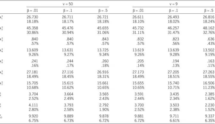
By assuming that the joint distribution of these ten random variables follows a multivariate normal dis-tribution, Panjer (2002) discusses the optimal alloca-tion problems for this data set. We assume that the joint distribution follows a multivariate Student-t dis-tribution with density function defined in Eq. (4.6). Since the original data is not available to us, we use
n = 9 and n = 50 for the data set, which represent small and large degree of freedoms, separately.
The total capital K is assumed to be 147 million, which is around one standard deviation of estimated means larger than the total sum of estimated means 134.13 million. This value is slightly larger than the VaR.95(S) = 145 based on n = 9, where S = X1
+ . . .+X10. Table 4 summarizes the optimal capital allocations for various scenarios based onq= .99.
From Table 4, it is observed that overall the larger risks are allocated with more capitals. It is seen from the covariance matrix thatX2 has the largest mean and variance, and it has a positive correlation with relatively large risks, say larger than 9 million, (X4,X6,X7), but it is uncorrelated withX1, and is negatively correlated withX10. Whenb is increasing, the capital requirement onX2 is increasing for both of n = 50 andn = 9; the capitals for X2 with n = 9 are larger than the corre-sponding ones with n = 50. This observation reflects that the model penalizes the large variance and heavy tail. For risksX1 andX6 with estimated means 25.69 and 24.05 millions, the capital requirements are 26.711 (18.17%) and 27.116 (18.45%) millions for CTE only increases from 50.60% to 51.58%. This
reflects the advantage of TMV model in quickly responding to a large risk level. It is also seen that the allocated capital for riskX3 based on the TMV model decreases by 2.78% while the allocated capi-tal based on the CTE decreases by 1.19% for X3. This is because the new TMV model takes into account the negative dependence betweenX2 andX3 for allocations. To conclude, compared to the other models, the new Model (1.2) has many desired prop-erties, such as reflecting the effects of dependence, and risk level.
4.4. Real data analysis
In this section, we analyze a real insurance data set presented in Panjer (2002). The total number of busi-ness lines is 10 with
, . . . , ,
1 10
( )
=
XT X X
which represent a range of insurance and other related financial products. The estimated mean vec-tor (million) is
25.69, 37.84, 0.85,12.70, 0.15, 24.05,14.41, 4.49, 4.39, 9.56 .
(
)
µ =
The correlation matrix was reported in Panjer (2002) and Valdez and Chernih (2003) reported the covari-ance matrix, which is reproduced here for the sake of convenience.
7.24 0 0.07 0.07 0.28 2.71 0.51 0.28 0.23 0.21
20.16 0.05 1.6 0.05 1.39 1.14 0.91 0.81 1.74
0.04 0 0.01 0.08 0.01 0.02 0.02 0.07
1.74 0.17 0.26 0.19 0.14 0.18 0.79
0.32 0.24 0.01 0.02 0.08 0.01
14.98 0.43 0.33 1.89 1.6
2.53 0.38 0.13 0.58 0.92 0.16 0.4 1.12 0.58 6.71
− − − −
− − −
− − − −
− −
− − −
− − −
−
− −
the works by Laeven and Goovaerts (2004), Dhaene et al. (2012), and Xu and Mao (2013), which capture both magnitude and variability of tail risks. As seen from the numerical evidence, the TMV model has many intriguing properties, such as penalizing the large risk, variance, positive dependence, and reflecting the tail risk level. It also provides many intuitive expla-nations on the optimal capital allocations. The penal-ization parameterb, which is either determined by the historical data or by the experience of the decision maker, provides an additional flexibility for controlling the tail variability. Since the analytical solutions for the TMV model is infeasible, we explore the general equa-tions which could be easily implemented in the software (R code is available upon request). It may be interest-ing to comprehensively compare the TMV model to those in the literature (Bauer and Zanjani 2013) and use the TMV model for DHS capital allocation. The preliminary study shows that the TMV model pro-vides some promising results, which is currently being pursued, and will be reported when it is completed.
n = 50, respectively. The capital requirement on riskX6
slightly decreases whenb changes from .01 to .5, which may be caused by the correlations with the other risks. For the case ofn =9, it is observed that the capital requirements for risksX1 andX6 both increase whenb
changes from .01 to .5, which may reflect the penalty on the variability again. It is interesting to observe that whenb changes from .01 to .1 withn = 9, the capital requirement on X1 is slightly less, while on X6 it is slightly more. It may be explained by noting that the variance ofX1 is less than that ofX6, and furtherX6
is positively correlated withX2. For riskX10, it is seen that it is negatively correlated with (X1,X2,X4,X6), and therefore, it is not surprising to observe that the capi-tal requirements all decrease whenb increases.
5. Conclusion
In this paper, we have suggested a new capital allo-cation rule which stems from the tail mean-variance premium calculation principle. It is also a variation of
Table 4. Optimal capital allocations (amounts and percentages) for various parameters based on TMV model (1.2) with a total capitalK 147 andq .99.
n = 50 n = 9
b = .01 b = .1 b = .5 b = .01 b = .1 b = .5
*k1* 26.730
18.18% 26.71118.17% 26.72118.18% 26.61118.10% 26.49318.02% 26.81618.24%
*k*2 45.358
30.86% 45.47630.94% 45.65531.06% 45.73231.11% 46.25731.47% 48.16232.76%
*k*3 .840
.57% .840.57% .843.57% .832.57% .823.56% .636.43%
*k*4 13.609
9.26% 13.6319.27% 13.7259.34% 13.6199.26% 13.6399.28% 13.5029.19%
*k*5 .241
.16% .244.17% .260.18% .205.14% .194.13% .163.11%
*k*6 27.181
18.49% 27.11618.45% 26.91618.31% 27.17318.49% 27.20518.51% 27.26318.55%
*k*7 15.705
10.68% 15.61510.62% 15.66110.65% 15.65510.65% 15.74010.71% 16.50611.23%
k*8 3.704
2.52% 3.6642.49% 3.5652.43% 3.5912.44% 3.4352.34% 2.3851.62%
k*9 4.111
2.80% 3.7932.58% 2.7921.90% 3.7002.52% 3.5032.38% 2.2301.52%
k*10 9.920
Therefore, it holds that
Var VaR
2 ECT .
1 1
1
1. 1 1
X k S S
k
F k k
q
S S
[
( ) ( )]
( ) ( )
∂ − >
∂ = −
+
Further, for anyj= 2, . . . ,n, we have
Cov , VaR
, VaR
ECT
I VaR
ECT
Cov , I VaR
ECT ECT
Cov , ,
1 1
1
1, 1 1
1. 1
1 1
1. 1
1 1
1. 1 1. 1
, 1
1
E
X k X k S S
k
x k f x x S S dx dx
F k k
X k X k S S
F k k
X k X k S S
F k k F k k
k k
j j q
j j j j q j
k k
S S j
j j q
S S j
j j q
S S j S S j
S j j
∫
∫
{
}
{
}
[
]
(
)
(
)
(
)
( )
(
)
( )
(
)
( )
( )
(
)
( ) ( ) ( ) ( ) ( ) ( ) ( ) ( ) ( ) ( ) ( )∂ − − >
∂
= − − >
+
= − − ≥ >
+
= − − ≥ >
− + = − + + ∞ ∞ + + +
where f1,j(., .S > VaRq(S)) is the joint density of [(X1,Xj)S> VaRq(S)]. Therefore, we have
2 ECT
2 Cov ,
2 ECT
2 ECT
2 Cov ,
2 Cov ,I
VaR 2 Cov ,
2 Cov , .
1
1. 1 1. 1 1
, 1
2
1. 1 1
1. 1 1
, 1
2
1. 1 1 1 1 1
, 1
2
1. 1 , 1
1
k
f
k F k F k k
k k
F k k
F k k
k k
F k X k X k
S S k k
F k k k
S S S
S j j n S S S S S j j n S
q S j
j n
S S j
j n
∑
∑
∑
∑
}
{
(
)
(
)
(
)
(
)
( ) ( ) ( ) ( ) ( ) ( ) ( ) ( ) ( ) ( ) ( ) ( ) ( ) ∂∂ = − − β
− β
= − − β
+ β
− β
= − − β − ≥
> − β
= − − β
+ = + = + + = + =
Forl= 1, 2, . . . ,n, it follows that
,
2 Cov , .
. ,
1
k
L
kl F k k k
l S l S j l
j n
∑
(
)
( )(
)
∂ λ
∂ = − − β = + − λ
6. Acknowledgment
The author thanks the editor and two anonymous reviewers for their constructive comments that helped to improve the presentation of this paper. In particular, Section 4.3 was added based on the suggestion from a referee. This work was partly supported by the Casu-alty Actuarial Society through the Individual Grants Competition.
Appendix
Proof of Theorem 2.1: Define
VaR
Var VaR ,
1
1
E k
f X k S S
X k S S
i i q
i n
i i q
i n
∑
∑
( ) ( ) ( ) ( ) ( )= − >
+ β − >
+ = + = and . 1
∑
( )= − = kh K ki
i n
Let
, .
k k k
L
(
λ =)
f( )+ λh( )According to Kuhn-Tucker theory (Bertsekas 1999), we need to solve the following equations, for
l= 1, . . . ,n,
,
0, , 0.
k k
(
)
(
)
∂ λ ∂ = ∂ λ ∂λ = L k L lWe first observe that
ECT , 1 1 1. 1 k
k F k
S S ( ) ( ) ∂ ∂ = − and E Var VaR
VaR ECT .
1 1
1 1 2 1 2
[
]
[
]
[ ] ( ) ( ) ( ) ( ) ( ) − >= − > −
+
+
X k S S
X k S S k
q