Managing Humanitarian Operations: The Impact of Amount, Schedules,
and Uncertainty in Funding
Karthik V. Natarajan
A dissertation submitted to the faculty of the University of North Carolina at Chapel Hill in partial fulfillment of the requirements for the degree of Doctor of Philosophy in the
Kenan–Flagler Business School (Operations).
Chapel Hill 2013
Approved by:
Dr. Jayashankar M. Swaminathan, Chair Dr. Adam Mersereau, Committee Member Dr. Dimitris Kostamis, Committee Member Dr. Ann Marucheck, Committee Member
Abstract
KARTHIK V. NATARAJAN: Managing Humanitarian Operations: The Impact of Amount, Schedules, and Uncertainty in Funding
(Under the direction of Dr. Jayashankar M. Swaminathan)
Acknowledgements
This dissertation would not have been possible without the support, advice and encouragement provided by faculty members at the Kenan-Flagler Business School, friends and colleagues both within and outside the school, and my family members.
My heartfelt thanks goes to my advisor, Dr. Jayashankar M. Swaminathan, whose guidance and mentorship has made the last few years a very rewarding experience. Working with Jay has developed my critical thinking and taught me the importance of looking at the big picture when working on different projects. His passion and commitment to research continues to amaze me and he has shown me, by example, the value of perseverance and a strong work ethic that are essential qualities to be a successful researcher. In many ways, he is my role model and I feel absolutely privileged to have had the opportunity to work with him. Jay, thank you.
My special thanks also go to Dr. Adam Mersereau and Dr. Dimitris Kostamis for agreeing to serve on my committee, and for their support over the years, beginning in the first year of the doctoral program. I am very grateful for their patience and guidance while working on my summer paper, and I hope that I will have the opportunity to collaborate with them again at some point in the near future. Adam, a special thank you to your family for inviting us to the annual Thanksgiving lunch. We very much enjoyed it.
class in my first year in the Ph.D. program.
I would like to thank my senior colleagues — Vidya Mani, Yen-Ting Lin, Gokce Esenduran, Olga Perdikaki and Sriram Narayanan for their help and advice regarding navigating the dif-ferent stages of the program. I will always cherish the friendship of Aaron Ratcliffe, Adem Orsdemir and Gang Wang, and I very much enjoyed the McColl Cafe and patio lunches we had together over the years. I would like to wish the upcoming doctoral students — Zhe Wang, Hyun Seok Lee and Ying Zhang the very best in successfully completing the program, and I look forward to hearing about their graduations. I would also like to extend my thanks to Virgnia Kay, Jyotishka Ray, Valmik Khadke, Kevin Miceli and Chang Hyun Kim for their friendship and support, and sharing many light moments.
Table of Contents
Table of Contents vi
List of Tables ix
List of Figures x
1 Introduction 1
2 Inventory Management in Humanitarian Operations 7
2.1 Introduction . . . 7
2.1.1 Literature Review . . . 9
2.2 Model . . . 10
2.2.1 Impact of Funding Timing . . . 16
2.2.2 Impact of Variability in Funding Timing . . . 17
2.2.3 Deterministic Funding Schedule . . . 19
2.3 Computational Study . . . 20
2.3.1 Deterministic Funding Schedules . . . 21
2.3.2 Stochastic Funding Schedules . . . 26
2.5 Conclusions and Managerial Insights . . . 31
3 Resource Allocation in Humanitarian Health Settings 33 3.1 Introduction . . . 33
3.1.1 Literature Review . . . 35
3.2 Model . . . 37
3.2.1 Patient Entry Dynamics . . . 39
3.2.2 Funding Inflows . . . 39
3.2.3 Objective Function . . . 40
3.3 Optimal Allocation Policy . . . 41
3.3.1 Monotonicity of the Optimal Policy . . . 42
3.3.2 Additional Monotone Properties of the Optimal Policy . . . 44
3.4 Heuristics . . . 47
3.4.1 Heuristic FCFS . . . 47
3.4.2 Heuristic PNS . . . 47
3.5 Impact of Funding Changes . . . 50
3.5.1 Expected Funding Timing . . . 50
3.5.2 Variability in the Funding Timing . . . 51
3.6 Computational Study . . . 53
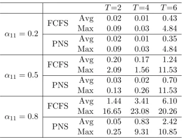
3.6.1 Performance of the Heuristics . . . 56
3.6.2 Impact of Transition Rates . . . 59
3.7 Conclusions and Managerial Insights . . . 65
4 Supply Vs. Demand Side Investment in Humanitarian Operations 70 4.1 Introduction . . . 70
4.2 Literature review . . . 73
4.3 Centralized model . . . 74
4.3.1 Impact of supply– and demand–side parameters . . . 76
4.3.2 Impact of Demand Changes . . . 81
4.4 Decentralized model . . . 85
4.4.1 Per–unit reimbursement rate contract . . . 87
4.4.2 Penalty–reward contract . . . 90
4.4.3 Comparison of the contracts . . . 92
4.5 Conclusions . . . 92
5 Conclusions and Future Research 94
A Proofs for results in Chapter 2 98
B Proofs for results in Chapter 3 112
C Proofs for results in Chapter 4 118
List of Tables
2.1 Average % cost difference for different funding patterns relative to ES funding . . 23
2.2 Average relative % cost difference as a function of CR . . . 23
2.3 Effect of demand variability for different funding patterns . . . 23
2.4 Average % cost difference for different funding patterns relative to NFC . . . 25
2.5 Number of installments considered for each N . . . 26
2.6 Average relative % cost difference due to funding uncertainty . . . 28
2.7 Effect of demand variability on the % cost difference due to funding uncertainty . 28 2.8 Average % cost difference for different funding patterns at different funding levels 29 2.9 Average relative % cost difference (relative to NFC) due to funding uncertainty . 29 3.1 Number of installments for eachT . . . 55
3.2 Performance of the heuristics relative to the optimal allocation policy . . . 57
3.3 Performance of the FCFS heuristic relative to the PNS heuristic . . . 57
3.4 Average running time . . . 58
3.5 Impact of transition rates at 50% funding level . . . 59
3.6 Impact of transition rates at 100% funding level . . . 59
3.7 Impact of transition rates at 150% funding level . . . 60
3.8 Impact of the number of installments at 50% funding level . . . 67
3.9 Impact of the number of installments at 100% funding level . . . 68
List of Figures
2.1 Average % cost difference for different funding patterns at different funding levels 24
2.2 Average % cost difference due to funding timing uncertainty . . . 28
4.1 Impact of θon s∗i . . . 79
4.2 Impact of oe ons∗i . . . 80
Chapter 1
Introduction
Against the backdrop of escalating costs, growing demand for health commodities, and tight-ening budgets, humanitarian organizations have come under increasing pressure to target aid financing effectively and justify the enormous levels of aid spending. Consequently, there is a growing interest within the humanitarian community to look at ways to improve the efficacy and efficiency of their operations. Although global health spending has increased tremendously in the last decade, many organizations like The Global Fund to Fight AIDS, Tuberculosis and Malaria, the Global Alliance for Vaccines and Immunization (GAVI Alliance) and the World Health Organization (WHO) face serious funding shortfalls. This situation is expected to fur-ther deteriorate in the current economic climate with many governments, including the U.S. and Spain, cutting down their foreign aid. In addition, global health funding is highly volatile and unpredictable — this is partially driven by the budget and funding cycles of the donors, some aspects of which are often outside their control.
the problems studied in the first two chapters comes from the ready–to–use–therapeutic–food (RUTF) supply chain in the Horn of Africa but the problems we study and the underlying issues are also relevant to many other humanitarian organizations operating in the global health sector.
In the first chapter, we study the problem of managing inventory of a health commodity in the presence of funding constraints over a finite planning horizon. Funding from donors, which finances the procurement, is received in installments throughout the planning period with uncertainty around both the timing and amount received. In the problem that motivated this study, the country office of UNICEF, which managed the RUTF procurement, was constrained by the timing of receipt of previously promised funding from donors. Given the highly variable and unpredictable nature of the inflow of funds, we (i) identify the optimal procurement strategy taking into account the current financial position as well as the funding due to arrive in the future, and (ii) quantify the impact of funding timing, funding level and funding uncertainty on the operating costs.
We model this problem using a stylized multi–period inventory model with financial con-straints. Among other results, we show that a capital–dependent modified base stock policy is optimal. Remarkably, we are able to show that the capital–dependent modified base stock policy can be simplified to a state independent policy, which greatly simplifies the implemen-tation of the optimal policy and enhances its appeal. We also prove several analytical results regarding the impact of funding uncertainty and increased variability in the funding timing.
moderated by the uncertainty in demand.
A key message of this research is that humanitarian supply chain managers need to consider the funding level as well as the operating environment while undertaking initiatives to improve the funding situation.
In the first chapter, one simplifying assumption we make is that a single dose/unit of the product suffices to meet the needs of a patient/customer. This assumption makes the model general enough to be applicable to a wide variety of products — e.g., malaria bed nets and reproductive health supplies like contraceptives — but a multi-dose framework is more appropriate in certain other settings. For example, in the outpatient treatment of severely malnourished children, the affected children are given Plumpy’Nut for several weeks until they are deemed fit. This multi-dose framework is also common in the treatment/prevention of many other diseases including certain types of vaccines.
In Chapter 2, we extend the work in the first chapter by relaxing the single dose assumption, and allow for the possibility that patients enrolled in a humanitarian health program could be in different health states requiring treatment over different lengths of time (corresponding to different amounts/doses of the product) before they are completely cured. The treatment duration and the response to treatment or non–treatment could also vary depending on the health state. In this setting, the problem of dynamic allocation of a scarce resource, which in our case is funding, between patients in different health states assumes significance. Given that the total available funding is limited and funding inflow is unpredictable, in certain situations, it might be beneficial to reserve a portion of the funding available on–hand to serve more severe patients in the future periods.
two health states respond to treatment and non–treatment in every period.
We use a multiperiod stochastic dynamic programming framework with health–state depen-dent per–period and terminal penalty costs to analyze the allocation problem. We characterize the optimal policy to be a state–dependent policy and we prove several monotonicity prop-erties that could help reduce the computational burden involved in determining the optimal policy. Despite the potential simplifications offered by the monotonicity results, determining the optimal policy is time–intensive for problems with long planning horizons. So we develop two heuristics (referred as PNS and FCFS heuristics) that can solve real–size problems fairly quickly. Our computational results suggest that the PNS heuristic performs well in terms of the solution quality and running time across a wide range of scenarios. The FCFS heuristic also performs well in many cases but it is less robust than the PNS heuristic and in certain settings, there is a noticeable performance gap between the two heuristics.
Our computational study also provides several insights regarding the impact of funding level and uncertainty in funding. We find that the impact of uncertainty in funding timing could be very different depending on the length of the planning horizon and the system funding level. For short–planning horizons, uncertainty in funding leads to a loss of disease–adjusted life months while in case of longer planning horizons, receiving the funding in fewer, lumpy installments involving more uncertainty in funding timing might be preferable only in under– financed systems ( < 100% funding level). In well–funded systems ( ≥ 100% funding level), having a smooth and predictable funding pattern is always preferred. This finding highlights the importance of taking into account the system characteristics when making funding–related decisions so as to maximize the per–dollar impact of funding provided to global health programs. Regarding the system funding level, we find that low funding availability leads to a significant loss of disease–adjusted life months in under–financed systems. Hence, it might be beneficial to receive additional funding even at the cost of increased funding uncertainty. In well–funded systems, the losses from the increased funding uncertainty outweigh the potential benefits from the additional funding, and hence less overall funding should not be traded for larger but more uncertain funding.
dilemma faced frequently faced by in–country public health managers. Low aid effectiveness and poor coverage have often been attributed to a combination of failures on both the demand and supply side. Supply–side factors determine the availability of essential health supplies and services when and where they are needed, and supply–side investments are geared to-wards reducing or eliminating supply chain inefficiencies that could lower product availability. Demand–side factors focus on the consumer, and investments on the demand–side are aimed at mobilizing demand for the service or product by increasing community awareness and elim-inating or reducing the social, economic and cultural barriers to access. While countries would ideally like to invest as much as possible on both sides, oftentimes they only have a limited budget to spend on interventions aimed at improving health outcomes. In light of the limited funding availability, choosing the right investment mix is critical since too much or too little supply could significantly affect program coverage.
on the program coverage. We find that higher mean demand may not necessarily imply higher coverage but a higher variability in the demand always leads to a lower coverage for many of the commonly used demand distributions.
Chapter 2
Inventory Management in
Humanitar-ian Operations
2.1
Introduction
Financial flows play an important role in humanitarian operations and impact their scope, ef-fectiveness and efficiency. While the total amount of donations received can impact the efficacy of such operations, the timing, predictability, and flexibility of usage around those funds also have a strong influence (Wakolbinger and Toyasaki 2011). In a global health context, unpre-dictability and delays in donor funding are often cited as the reasons behind impaired supply chain management and reduced coverage (Fininnov 2011). A recent study by the Brookings Institution (Lane and Glassman 2008) estimates that for every dollar received in funding, 7 to 28 cents is lost due to funding delays.
little systematic information is available on the magnitude of the predictability problem and thus its potential impact on aid recipients.”
Motivated by the ready–to–use therapeutic food (RUTF) supply chain in Africa, we study the problem of managing inventory of a nutritional product in the presence of funding con-straints over a finite horizon (Swaminathan 2009, 2010). Funding is received in installments throughout the planning period with uncertainty around the timing and amount. This un-predictable nature of donor funding is typical of the funding situation in many global health programs. Even in the best of situations there might be uncertainty in terms of timing of the receipt of those installments. In the problem that motivated this study, the country office of UNICEF that had to procure RUTF were constrained by the timing of the receipt of previously promised funding from donor agencies. Given the highly variable and unpredictable nature of the inflow of funds, an important question that arises is how to effectively manage inventory, taking into account both the current financial position as well as the funds that are due to arrive in the future periods.
In this chapter, we model the above situation with a multi–period stochastic inventory model with financial constraints. Our goal is to (i) determine the optimal ordering policy given the complexities associated with the funding and (ii) characterize the impact of funding timing, funding level, and funding uncertainty on the operating costs. Among other results, we show that despite the uncertainty in funding, the optimal replenishment policy is a state– independent modified base stock policy, which greatly enhances the appeal and implementation of the optimal policy. We also prove that uncertainty in funding timing (in comparison to a deterministic financial schedule) increases operating costs and so does the stochastically domi-nated late arrival of funds. Finally, we also show that increased variability in the funding timing (as measured by convex ordering) leads to higher costs.
funding (where a major chunk of the total funding is received in the later periods), (2) the interaction between funding level (total funding received as a % of the amount required to meet total expected demand) and funding pattern, (3) the effect of uncertainty in funding timing and, (4) the relative importance of funding level and pattern vis a vis funding uncertainty.
Among other results, we provide the following computational insights. (1) Avoiding funding delays should be a top priority for humanitarian supply chain managers. In case of deterministic funding schedules, while evenly–spread funding facilitates planning, it is not the optimal funding pattern due to its inability to accommodate large demand surges upfront; (2) Front–loading the funding brings significant benefits in under–financed systems (<100% funding level) while avoiding back–loading is critical in fully–financed systems (100% funding level). (3) Front– loaded funding at 75% funding level is better than back–loaded funding at 100% funding level. Depending on the level of front– and back–loading at 75% and 100% funding levels, the operating costs under back–loaded funding at 100% funding level vary between 1.5–5.5 times the operating costs under front–loaded funding at 75% funding level; (4) There is a non-linear increase in costs with increased uncertainty in funding. Further, this effect decreases with demand uncertainty.
2.1.1 Literature Review
Our work is related to three streams of literature.
Inventory Management under Capacity Constraints: Financial constraints on pro-curement are somewhat similar to supply–capacity constraints and a lot of work has been done on inventory management under capacity constraints (see Federgruen and Zipkin 1986 a,b, Ka-puscinski and Tayur 1998, Aviv and Federgruen 1997, Ciarallo et al. 1994, Wang and Gerchak 1996). The main difference between these models and ours is that while physical capacity constraints are rigid, financial constraints can be made flexible. Unlike production capacity, unused capital does not go waste and can be utilized in the future periods.
Humanitarian Operations: Our paper also contributes to the growing body of work on humanitarian operations. Within humanitarian operations, a majority of the papers focus on disaster relief, e.g., Duran et al. (2011) and Beamon and Kotleba (2006) focus on inventory management during emergencies. In recent years, long-term public health issues have also received attention from the operations management community, e.g., Taylor and Yadav (2011), Rashkova et al. (2011) and Deo and Sohoni (2011). However, we believe that ours is the first work to look at inventory management from a humanitarian health perspective. In addition, to the best of our knowledge, Rashkova et al. (2011) and our work are the only ones to focus explicitly on the role of funding in humanitarian operations.
The rest of the chapter is organized as follows: In section 2, we introduce the model and provide analytical results regarding the optimal policy and the impact of funding. In section 3, we present the results of our numerical study and discuss the impact of funding on operating costs. In section 4, we demonstrate that the inventory replenishment policy established in section 2.2 is optimal under more general settings. We offer some managerial insights and conclude the chapter in the last section.
2.2
Model
We consider a finite–horizon, periodic–review inventory model for a single product. The plan-ning horizon is divided intoNperiods with the time indexing done in the reverse order, i.e., the first period is period N, followed by N-1, N-2 and so on. Demands in successive periods, ζt,
distribution function ft and cumulative density function Ft. The system is financed through external funding received in m ≤ N installments. The installment sizes (amount received in each installment) are known beforehand but the time of receipt of each installment could be uncertain. We refer to a funding scenario with uncertain funding timing as astochastic funding schedule. A special case of thestochastic funding schedule is a scenario where both the install-ment amounts and timing are known beforehand. We refer to this special case scenario as a
deterministic funding schedule.
We denote the funding vector by Z = (z1, z2, z3, ..., zm) where zm and z1 are the first and last installments received respectively. Therefore, the total funding received over the planning horizon is
m
X
j=1
zj. For our analysis, we do not impose any restrictions on the installment sizes
— the amount received in each installment could be very different from one another. Let cbe the unit purchase cost, hdenote the unit holding cost per period andbbe the penalty cost per unit per period for any unsatisfied demand. We make the following assumptions in our model.
1. Unmet demand is completely backlogged. While this is an approximation in the RUTF context, the backlogging assumption is valid for a variety of health commodities, e.g., malaria bed nets and reproductive health supplies like contraceptives.
2. All the installments are received before the end of the planning horizon. As we mentioned before, donors make a commitment based on the funding proposals and while the amount in the individual installments may vary based on the donors’ budget cycles, in most cases, the committed amount is received in full before the end of the planning period for which the donation was sought.
3. Borrowing capital is not an option. In the application that motivated this study, country offices place procurement orders only when they have raised enough money from the donors to fund the procurement. Currently, they neither borrow money to finance the procurement nor do they have access to a credit line.
assumption in the context of the problem that motivated this study but it makes the model general enough to be applicable to a wide variety of humanitarian health programs.
The sequence of events in any given periodtis as follows: 1. Funding (if any) is received at the start of period t. 2. Procurement decisions are made, subject to capital available on–hand. We assume that replenishments arrive instantaneously. (This assumption is only for simplicity and in section 4, we demonstrate that relaxing this assumption does not change the structure of the optimal replenishment policy.) 3. Finally, demand is realized and holding and backorder costs are calculated based on the ending inventory.
Let xt,yt denote the on–hand inventory before and after ordering in periodt andrtbe the capital available at the start of period t, after receiving installments (if any) in period t. The state variable Ot keeps track of the number of outstanding installments as of the beginning of period t, after receiving installments (if any) in that period. The recursive equation for
rt is thus given by rt = rt+1 −c(yt+1 −xt+1) + Ot+1
X
j=Ot+1
zj. We let Pt(i) denote a random
variable corresponding to the number of outstanding installments at the beginning of period
t−1, given that the number of outstanding installments at the beginning of period t is i.
PN+1(m) is the number of outstanding installments at the beginning of periodN. Also, define
Pt(i, j)≡P r(Pt(i) =j).
Then, for a fixed funding vectorZ, the optimality equations are given by
Jt(xt, rt, Ot) = min yt∈[xt,xt+rtc]
c(yt−xt) +bEζt[ζt−yt]
++hEζ
t[yt−ζt]
+
+EOt−1EζtJt−1(yt−ζt, rt−c(yt−xt) +
Ot
X
j=Ot−1+1
zj, Ot−1)
(2.1)
Since all the installments are received before the end of the horizon,O1=0 always. The terminal cost isJ0(x0, r0,0) = 0∀(x0, r0).
Some intuitive properties of the cost–to–go function can be readily proven. For example, given xt,Ot and funding vector Zt,Jt(xt, rt, Ot) is monotone decreasing inrt. Additionally, if
Ot =k for some constant k, zi1 = zi2 ∀ i= 1,2, ..k−1 and z2k−zk1 =rt1−rt2 =K ≥0, then
Jt xt, r2t, Ot|Zt2
≥Jt xt, r1t, Ot|Zt1
, i.e., it is more valuable to have an extra dollar today than receiving it in the next installment.
Our first key result is the joint convexity of the value function in state variables xt and rt for fixedOt and Zt. We prove this in Lemma 1. The proofs for all the results in this chapter can be found in Appendix A.
Lemma 1. Jt(xt, rt, Ot) is jointly convex inxt andrt for fixed Ot and funding stream Zt.
In our analysis, we find it convenient to use a modified value function expressed in terms of variables xt and Rt=rt+cxt. Define
ˆ
Ct(yt, Rt, Ot) =cyt+bEζt[ζt−yt]
++hE
ζt[yt−ζt]
+
+EOt−1EζtJt−1(yt−ζt, Rt−cyt+
Ot
X
j=Ot−1+1
zj, Ot−1) (2.2)
Then, in terms of ˆCt, we have
(P1) ˜Jt(xt, Rt, Ot) =Jt(xt, rt, Ot) =−cxt+ min yt∈
h
xt,Rtc
i
ˆ
Ct(yt, Rt, Ot)
(2.3)
demon-strate that the optimal replenishment policy is actually simpler — the optimal policy is a state–independent modified base stock policy where the order up–to levels depend only on t
and not on Rt, Ot or the future funding streamZt.
To be precise, consider a multi–period inventory management problem with the same cost and demand parameters as problem P1 (see equation (2.3)), but no financial constraints. Let
N Vt(xt) be the minimum expected cost withtperiods to go, corresponding to this setting with no financial constraints. Then,
(P2) N Vt(xt) = min yt≥xt
c(yt−xt) +bEζt[ζt−yt]
++hE
ζt[yt−ζt]
++E
ζtN Vt−1(yt−ζt)
Let N V0(x0) = 0 ∀ x0. It is well known that a base stock policy is optimal for problem P2 and there exists an optimal base stock level yt∗ in each period such that if the inventory level in periodtis belowyt∗, it is optimal to order up–toy∗t, and not order otherwise. In Theorem 1, we prove that the unconstrained base stock levels yt∗, yt∗−1, ..., y∗1, optimal for problem P2, are optimal for problem P1 with funding constraints as well.
Theorem 1. Let yt∗, yt∗−1, ..., y∗1 be the optimal base stock levels corresponding to problem P2.
Let (xt, Rt, Ot) be the state of the system in problem P1 at the beginning of period t. Then, the
optimal ordering policy for problem P1 has the following simple structure.
Order up–toRt/c if Rt/c≤y∗t
Order up–toyt∗ if Rt/c > y∗t, xt< yt∗ and
Do not order if xt≥yt∗.
(2.4)
period t and the end of the horizon is solely determined by the sum: c×(on–hand inventory) + capital available on–hand + future funding. A closer look reveals that this sum is also independent ofOt. Hence, while the actual costs incurred might vary depending on the number of outstanding installments Ot, the incremental difference in costs obtained by changing the order quantity remains the same, irrespective of how many installments are outstanding.
A related question is why is the base–stock level independent ofRt? Recall thatRt(=cxt+rt) determines the maximum inventory level attainable in periodt. From a single–period perspec-tive, Rt acts like a production capacity constraint. In the presence of capacity constraints, it is well known that the (capacity–dependent) order up–to levels in each period are higher than the corresponding unconstrained base stock levels (see e.g., Federgruen and Zipkin 1986 a,b). So why is the optimal policy different for our problem with funding constraints ? The key reason is that, although both funding and capacity constraints place an upper bound on the order quantity in each period, there is a fundamental difference between the two. While unused capacity goes waste, unused capital can be used in the later periods, i.e., it acts like transferable capacity. Intuitively, this is the reason why the unconstrained base stock levels continue to be optimal even in the presence of funding constraints. This greatly enhances the appeal and im-plementation of the optimal policy since the state–independent base stock levels can be easily computed using techniques like IPA (see Glasserman and Tayur 1995). Additionally, the fact that the target inventory level is not tied to the future inflow of funds also makes operations planning easier since purchasing decisions depend only on the current state of the system and not on any future unobservable quantities.
2.2.1 Impact of Funding Timing
Throughout this section, we fix the funding vector Z = (z1, z2, ..., zm) and vary only the time of receipt of each installment. Recall that Pt(i) denotes a random variable corresponding to the number of outstanding installments at the beginning of period t−1, given that the number of outstanding installments at the beginning of periodtisi. Consider random variables
Pt1(i), i ∈ {0,1,2, ..., m} andPt2(i), i ∈ {0,1,2, ..., m} corresponding to funding scenarios 1 and 2 such that
Pt2(i)≥st Pt1(i) ∀ i∈ {0,1,2, ..., m} and ∀t∈ {2,3, ..., N} and (2.5)
Ptn(i0)≥st Ptn(i) ∀ i∈ {0,1,2, ..., m−1}, i
0 > i, n∈ {1,2} and∀ t= 2, ..., N (2.6)
where≥st means first–order stochastic dominance. The following is the definition of first–order stochastic dominance.
Definition 1. (Shaked and Shanthikumar 2007) Let X and Y be two random variables such
thatP(X > x)≤P(Y > x) for allx ∈ (−∞,∞). Then X is said to be smaller thanY in the usual stochastic order.
Condition (2.5) implies that the number of outstanding installments at the beginning of any period t is (stochastically) larger under funding scenario 2. Condition (2.6) says that, under both funding scenarios, the number of outstanding installments at the beginning oft−1 stochastically increases in the number of outstanding installments at the beginning of period
t. We denote the value functions associated with random variables Pt1 and Pt2 by Jt1 and Jt2
respectively. In the following theorem, we demonstrate that the (stochastically) early arrival of funds offers increased procurement flexibility, resulting in lower operating costs.
Theorem 2. If conditions (2.5) and (2.6) hold, then Jt2(xt, rt, j) ≥ Jt1(xt, rt, j) for every
2.2.2 Impact of Variability in Funding Timing
Having established that ‘earlier is better’ (in a stochastic sense) when it comes to the funding timing, we now focus our attention on the variance aspect of the uncertainty in funding. For a fixed funding vector, we compare two funding scenarios; in the first, there is high variability around the number of outstanding installments at the beginning of any given period while there is relatively less variability in the second. More specifically, we represent the two funding scenarios by random variablesPt1(i), i ∈ {0,1,2, ..., m} andPt2(i), i ∈ {0,1,2, ..., m} such that
Pt2(i)≥cvxPt1(i) ∀ i∈ {0,1,2, ...m}and t= 2,3, ..., N (2.7)
{Pn
t(i), i ∈ {0,1,2, ...m}} ∈SICX, n= 1,2 (2.8)
Condition (2.7) states that Pt2(i) is larger than Pt1(i) in the convex order. The following is the definition of a convex order.
Definition 2. (Shaked and Shanthikumar 2007) Let X and Y be two random variables such
thatE[φ(X)]≤E[φ(Y)] for all convex functionsφ:R→R. Then X is said to be smaller than
Y in the convex order.
Condition (2.7) implies that Pt2(i) is more variable than Pt1(i) but, EPt2(i) =EPt1(i). The convex ordering helps us to isolate the impact of variability around the funding timing since the mean number of outstanding installments remains the same under scenarios 1 and 2. Con-dition (2.8) states that{Pn
t (i), i ∈ {0,1,2, ...m}}, n= 1,2 belong to the class of stochastically increasing convex family of distributions.
Definition 3. (Shaked and Shanthikumar 2007) Let{X(θ), θ∈Θ}be a set of random variables. Then
2. {X(θ), θ ∈Θ} ∈ SICX (stochastically increasing and convex) if {X(θ), θ ∈ Θ} ∈ SI and Eφ(X(θ)) is increasing convex inθ for all increasing convex functions φ.
The following property can be used to check the SICX property for discrete random vari-ables.
Property 1. (Shaked and Shanthikumar 2007) Suppose that for each θ ∈ Θ, the support of
X(θ) is in N. Then, {X(θ), θ ∈ Θ} ∈ SICX if, and only if, {X(θ), θ ∈ Θ} ∈ SI and
∞
X
l=k
P r{X(θ)≥l} is increasing convex inθ for all k∈N.
A number of known distributions satisfy the SICX property. For example, if X(µ, σ) is a normal random variable with mean µ and standard deviation σ, then, for each σ > 0,
{X(µ, σ), µ ∈R} ∈ SICX. Similarly, if X(λ) is a Poisson random variable with mean λ, then
{X(λ), λ ∈ [0,∞)} ∈ SICX. Another example could be a random variable X(n), which is uniformly distributed on{0,1,2, ..., n−1}. Then,{X(n), n∈N+} ∈SICX.
In the following lemma, we demonstrate that, for any {Pt} satisfying condition (2.8), the minimum expected cost with t periods to go is increasing and convex in the number of out-standing installments at the beginning of t, provided the funding vector Z is front–loaded. We refer to a funding vector Z as front–loaded if Zi ≤Zi+1, i= 1,2, ..., N −1 and back–loaded if
Zi ≥Zi+1. Notice that a funding vector with equal installments also satisfies the definition of a front–loaded funding vector.
Lemma 2. Let Z be a front–loaded funding vector and condition (2.8) hold. Then, Jt(xt, rt+ i
X
k=j+1
zk, j) is increasing convex in j for j≤iwhere i∈ {0,1,2, ...m}.
We should point out that front–loaded funding is a sufficient but not necessary condition for the above result to hold. Our final result characterizes the impact of variability in the funding timing—given that the expected number of installments received remains the same, a higher variability around the number of outstanding installments at the beginning of any given period drives up the operating costs and results in poor performance.
Theorem 3. LetZ be a front–loaded funding vector and conditions (2.7) and (2.8) hold. Then,
2.2.3 Deterministic Funding Schedule
As we mentioned before, the deterministic funding schedule is a special case of the stochastic funding schedulewhere both the installment amounts and the time of receipt of each installment are known. Under a deterministic funding schedule, without loss of generality, we can assume that funding is received in every period (i.e., exactly inN installments) with some installments possibly being 0. Let Vt(xt, rt|Zt) be the minimum expected cost witht periods to go under a deterministic funding schedule, given state variables xt, rt, and the future funding vectorZt. Since we receive an installment every period, there is no need to keep track of the number of outstanding installments in case of a deterministic funding schedule. As with stochastic funding schedules, we will explicitly condition onZtonly when we compare different funding schedules.
In sections 2.2.1 and 2.2.2, we fix the funding vector, and explored one part of our second main research question: how does the uncertainty and variability in the funding timing impact operating costs? Using deterministic funding schedules, our goal is to fix the funding timing and explore the other part of our second research question: what is the impact of funding amount and funding schedules as relates to operating costs? Specifically, we are interested in answering the following questions: 1. Does an increase in the total funding received over the horizon necessarily lead to better performance? 2. Given that the total funds received over the
horizon remains the same, does advancing additional funds to a certain period have the same
level of impact as delaying the same amount until the next period?
Consider two deterministic funding schedules Z1 and Z2 such that
N−i
X
j=N
z1j ≥
N−i
X
j=N
z2j, i= 0,1, , ..., N−1 (2.9)
In Proposition 1, we show that an increase in total funding is guaranteed to result in lower operating costs if condition (2.9) holds.
Proposition 1. If condition (2.9) holds, then for anyxN ∈R,VN2(xN, r2N)≥VN1(xN, r1N).
Consider two funding vectors, Z1 and Z2 such that N
X
i=1
Zi1 = N
X
i=1
andZi1=ZN2−i+1, i= 1,2, ..., N, then clearly,Z2 is back–loaded. In this case, a direct applica-tion of the above proposiapplica-tion shows that for a fixed amount of total funding, the front–loaded vector Z1 is guaranteed to perform at least as well as the back–loaded vectorZ2. This result is on expected lines — what would be more interesting is to compare the following two funding scenarios: receiving less total funding, say $10 M, in a front–loaded fashion vs. receiving more total funding, say $ 20 M, in a back–loaded fashion. In this case, it is not clear whether the ad-ditional funding received leads to lower operating costs — we explore this in our computational study.
Next, we compare three deterministic funding vectors, Z = (z1, z2, ..., zt−1, zt, ...zN), ZA= (z1, z2, ..., zt−1 −δ, zt+δ, ..., zN) and ZD = (z1, z2, ..., zt−1 +δ, zt−δ, ..., zN). Let Vt, VtA and
VtD be the value functions associated with the three funding vectors respectively. We have the following result.
Proposition 2. VND(xN, rN)−VN(xN, rN)≥VN(xN, rN)−VNA(xN, rN) ∀ xN, rN.
Proposition 2 implies that the cost savings resulting from advancing additional funds to a certain period does not match the extra cost incurred if the same amount were to be delayed by one period. In essence, funding delays hurt more than the benefits from receiving funding early.
2.3
Computational Study
2.3.1 Deterministic Funding Schedules
Experimental Setup:
The numerical study was conducted for planning horizon, N, of different lengths, N =2, 4, 6, 12 and 24. The unit purchase cost c was normalized to 1 in all numerical experiments. For each N, we varied the following parameters.
Holding Cost: We chose four values for holding cost, h=0.01, 0.05, 0.1 and 0.25.
Penalty Cost: For each value of h, the penalty cost was varied so that the critical ratio (CR), (b−c)/(b+h), took on values 0.2, 0.4, 0.6, 0.8, 0.9 and 0.95 respectively.
Demand: In our work, we consider uniform and truncated normal demand distributions. To test the impact of demand variability on the operating costs, we considered U ∼[70,130] and
U ∼[25,175] for the uniform demand case. For truncated normal demand, the mean was fixed at 100 units and we used CV values of 0.1 and 0.25. The normal distribution was truncated at 3 standard deviations. Thus, for eachN, we have 4*6*4=96 problem instances.
Funding Patterns: For each combination of N, h, b and demand distribution, we consider five different funding patterns and four funding levels. The five funding patterns are extremely front–loaded funding (EFL), moderately front–loaded funding (MFL), evenly–spread funding (ES), moderately back–loaded funding (MBL) and extremely back–loaded funding (EBL). The holding cost and the funding patterns were chosen so as to be consistent with an earlier study that analyzes the state of the RUTF supply chain in the Horn of Africa (UNICEF 2009). For the backorder costs, due to lack of precise estimates, we decided to carry out a sensitivity analysis over a wide range of critical ratios. For all the funding vectors, the total funding received remained the same and is equal toN*funding level*mean demand. In our experiments, we consider 25%, 50%, 75% and 100% system funding levels and we label them as severely under–financed, moderately under–financed, mildly under–financed and fully–financed systems respectively. For example, a severely under–financed system receives N*0.25*mean demand over the entire planning period. For illustration purposes, we use the specific case of N=4,
different funding vectors.
EFL: The entire funding (=N*mean demand) is received upfront, i.e., the funding vector is (0, 0, 0, 400). Recall that we count time in the reverse order.
MFL: In the firstN/2 periods, the installment size is 1.5*mean demand followed by 0.5*mean demand in the lastN/2 periods. For the specific case considered, the funding vector is (50, 50, 150, 150).
ES: Every installment is equal to mean demand, i.e., the funding vector is (100, 100, 100, 100).
MBL: In the firstN/2 periods, the installment size is 0.5*mean demand followed by 1.5*mean demand in the lastN/2 periods. The funding vector would be (150, 150, 50, 50).
EBL: The entire funding is back–loaded to the last period, i.e., the funding vector is (400, 0, 0, 0).
Notice that as we move from EBL to EFL funding, more and more funds are received in the initial periods. Compared to ES funding, the front–loaded vectors can be considered as funding advances and back–loading can be considered as a funding delay. By using ES funding as a benchmark, we investigate how back–loading and front–loading the funding impacts operating costs.
Impact of Funding Pattern
We use the cost incurred under ES funding as a benchmark and compute the relative percentage cost difference for a particular funding pattern, say EBL funding, as follows: 100*(costEBL−
costES)/costES. Table 2.1 provides the relative percentage cost difference (relative to ES
fund-ing) for different funding patterns at 100% funding level, averaged over the 96 problem instances.
EBL MBL MFL EFL
N=2 152.54 69.42 -13.23 -13.69
N=4 425.68 126.30 -23.10 -24.89
N=6 664.40 178.97 -28.63 -30.76
N=12 1269.97 318.55 -37.61 -39.86
N=24 2230.19 547.26 -46.22 -48.30 Overall average 948.56 248.10 -29.76 -31.5
Table 2.1: Average % cost difference for different funding patterns relative to ES funding
premiums due to funding delays and utilize valuable aid dollars to increase coverage. However, it is not the optimal funding pattern since, under ES funding, there is very little flexibility to deal with large demand surges upfront. This is where an additional funding influx in the initial periods proves valuable. Relative to ES funding, the moderate shift in funds to the initial periods (MFL funding) results in average (averaged over all N) savings of 29.8%. However, pushing more and more funds to the initial periods yields little to no return and, even in case of an extreme push (EFL funding), the average savings is only 31.5%.
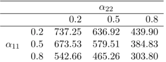
Also, notice that the gulf between front–loaded and back–loaded vectors increases with hori-zon length (Table 2.1) and critical ratio (Table 2.2) while it decreases with demand variability (Table 2.3). More interestingly, Table 2.3 also tells us that the benefits from front–loaded funding increase with the demand variance while the negative impact of a funding back–load is mitigated by the increased demand variability.
critical ratio
0.2 0.4 0.6 0.8 0.9 0.95
EBL 265.88 342.74 476.63 726.81 1094.32 1385.91 MBL 71.89 92.84 129.35 196.14 297.75 377.25 MFL -9.50 -12.58 -17.99 -30.69 -43.13 -55.01 EFL -9.76 -12.94 -18.52 -31.92 -44.41 -56.65
Table 2.2: Average relative % cost difference as a function of CR forN=6,U ∼[70,130] demand distribution and 100% funding level
EBL MBL MFL EFL
U ∼[70,130] 1020.73 268.76 -29.07 -29.85
U ∼[25,175] 554.96 133.46 -36.14 -40.52
N ∼[70,130] 1392.03 378.07 -21.90 -22.05
N ∼[25,175] 826.50 212.11 -31.92 -33.58
Funding Level vs. Funding Pattern
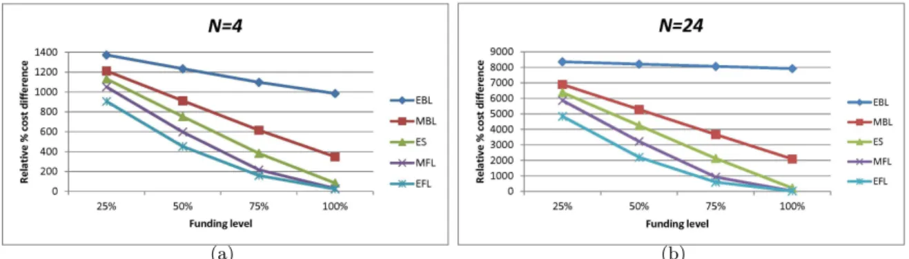
Having analyzed the impact of funding pattern on operating costs, we now proceed to under-stand the interaction between funding level and the funding pattern. We are mainly interested in understanding the relative importance of level of funding vis–a–vis funding pattern. Fig-ure 2.1 displays the relative percentage cost difference at different funding levels, ranging from severely under–financed to fully–financed. Here, we use the cost incurred under no funding constraints (NFC) as the benchmark to compute the relative percentage cost difference.
From Figure 2.1, we see that at very low funding levels (25% and 50% funding levels), the funding pattern is inconsequential — 100% funding level almost always outperforms. For a mildly under–financed system, the results are drastically different. From Figure 2.1, we see that back–loaded funding at 100% funding level performs significantly worse compared to front– loaded funding at 75% funding level. However, ES funding at 100% funding level outperforms even EFL funding at 75% funding level. This demonstrates that, at reasonably high funding levels, funding pattern is critical to system performance and a further increase in overall funding should not be traded for a delay in funding.
(a) (b)
Figure 2.1: Average % cost difference for different funding patterns at different funding levels
with maximum benefits seen either in moderately or mildly under–financed systems. The least benefits of front–loading are observed at 100% funding level. An intuitive reasoning for the U–shaped pattern is as follows: for severely under–financed systems, the total amount pushed to the initial periods is relatively less and in fully–financed systems, there is sufficient cash already available in the system for the additional funding to make a large impact.
In case of back–loaded funding, the additional cost incurred due to the delayed receipt of a majority of the funds is monotonically increasing in the funding level. The monotonicity result can be explained as follows: when funding is back–loaded, a major portion of the operating costs can be attributed to backorders. As the funding level increases, the difference between the funds available in each period under the evenly–spread and back–loaded funding scenarios also increase. This implies that the additional backorders ascribed to a funding delay also increase with the funding level.
Impact of Funding Constraints
Most global health programs are already financially constrained, a situation that is only ex-pected to worsen in the near future (Stokes 2011). The numbers in Table 2.4 offer some insights into the role of funding constraints. By taking difference of the relative percent-age cost differences in Table 2.4, we get 100*(costEBL −costES)/costN F C=2805.93, while 100*(costES −costN F C)/costN F C=121.18. This demonstrates that, as we move from EBL funding to NFC, a majority of the resultant benefits actually stem from reducing funding de-lays (making the funding even) and only a relatively small portion of the cost savings are attributed to the unlimited funding availability. Recall that NFC refers to a schedule where funding is never a constraint. The same insight also holds for MBL funding.
EBL MBL ES MFL EFL
2927.11 834.39 121.18 27.70 21.34
Table 2.4: Average % cost difference for different funding patterns relative to NFC at 100% funding level
access to unlimited funding is practically unrealistic and our study shows that front–loaded funding compares favorably with unlimited funding. Thus, even with limited funding, it is possible to achieve reasonable system performance as long as “enough” funding can be secured in the initial periods.
2.3.2 Stochastic Funding Schedules
Experimental Setup
Except for funding patterns, all other elements of the experimental set up remain unchanged from the deterministic funding case. As we mentioned in section 2.2, funding is received in
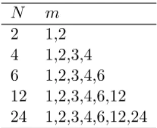
m≤N installments. For a fixed N, we consider several values ofm for the stochastic funding case, details of which are given in Table 2.5.
N m
2 1,2
4 1,2,3,4 6 1,2,3,4,6 12 1,2,3,4,6,12 24 1,2,3,4,6,12,24
Table 2.5: Number of installments considered for each N
For the stochastic funding case, we assume that the funding level is 100%, i.e., the total funds received over the entire planning horizon is fixed and is equal toN*mean demand in each period. To capture the uncertainty in the funding timing, we vary the number of installments. Depending on the number of installments (m) received, the amount received in each installment varies (=N/m*mean demand in each period).
1/16 while the probability of a more evenly spread funding vector like (200,0,200,0) increases to 1/8. Hence, the idea is that, as we increase the number of installments, the probability of the funding being more smooth and evenly spread out increases, thereby reducing the volatility in funding received until any given period.
Impact of Funding Uncertainty
We begin by discussing a result that is intuitive and holds true for all problem instances: reduc-ing the fundreduc-ing volatility, and makreduc-ing the fundreduc-ing more smooth and evenly spread out lowers
operating costs (see Figure 2.2). However, such benefits of reducing the funding uncertainty show diminishing rates of return, i.e., as the number of installments in which funding is cur-rently received increases, the marginal value of receiving the funding in an additional installment decreases.
To understand why reducing funding uncertainty leads to lower expected operating costs, consider the case where m=1 and N=6. The single installment could be received in any of the six periods and all possibilities are equally likely. Of course, there is nothing better than receiving the installment in the very first period (probability 1/6) but we also need to take into account the other possibilities (including an extreme back–loading with probability 1/6). Considered together, receiving funding in one installment is no longer the ideal scenario — in fact, it is the worst. In general, when the number of installments decreases, i.e., funding becomes more uncertain, it increases the possibility of the funding vector being moderately or severely back–loaded. Under uncertain funding, the possibility of the funding vector being front–loaded also exists but the non–linear increase in costs as we move from front–loaded to back–loaded funding means that the overall impact of the funding uncertainty is negative, i.e., in expectation, the operating costs increase.
Figure 2.2: Average % cost difference due to funding timing uncertainty
the funding uncertainty might outweigh the benefits. critical ratio
0.2 0.4 0.6 0.8 0.9 0.95
m=1 39.19 45.91 55.42 69.90 80.43 86.98
m=2 17.83 20.89 25.21 31.81 36.59 39.58
m=3 9.49 11.12 13.42 16.93 19.48 21.06
m=4 5.14 6.02 7.26 9.16 10.54 11.40
Table 2.6: Average relative % cost difference due to funding uncertainty (relative to a funding schedule withm=N) as a function of CR for N=6 andU ∼[70,130] distribution
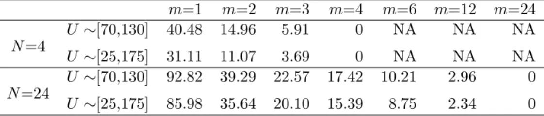
m=1 m=2 m=3 m=4 m=6 m=12 m=24
U ∼[70,130] 40.48 14.96 5.91 0 NA NA NA
N=4
U ∼[25,175] 31.11 11.07 3.69 0 NA NA NA
U ∼[70,130] 92.82 39.29 22.57 17.42 10.21 2.96 0
N=24
U ∼[25,175] 85.98 35.64 20.10 15.39 8.75 2.34 0
Table 2.7: Effect of demand variability on the average relative % cost difference due to funding uncertainty (relative to a funding schedule withm=N)
Funding Level vs. Funding Uncertainty
In this section, we aim to address our last but nevertheless, an important question: which of the two hurts system performance more — funding level or funding uncertainty ? To answer this question, we compare deterministic funding patterns at different funding levels to stochastic funding at 100% funding level. The results forN=24 are provided in Tables 2.8 and 2.9. The results are very similar for other values ofN.
hurts performance, making even the most uncertain funding (m=1) at 100% funding level attractive in comparison in almost all cases (an exception being EFL funding at 50% funding level).
Funding level EBL MBL ES MFL EFL
25% 8357.25 6894.14 6377.74 5861.40 4837.84 50% 8208.85 5282.63 4250.12 3220.79 2200.73 75% 8060.46 3671.19 2125.99 923.60 596.72 100% 7917.89 2086.40 213.73 26.65 16.80
Table 2.8: Average relative % cost difference for different deterministic funding patterns at different funding levels
For 75% funding level, the results are very different (compare row 3 in Table 2.8 with Table 2.9). While the back–loaded vectors at 75% funding level perform significantly worse than even the most uncertain funding at 100% funding level, front–loaded funding at 75% funding level outperforms uncertain funding at 100% funding level, even when the uncertainty is considerably reduced (m=24). This demonstrates that at relatively high funding levels, the choice between deterministic funding and an even larger overall but uncertain funding is not obvious — the answer depends on the deterministic funding pattern and the level of uncertainty in the larger overall funding.
2.4
Generalization to Positive Lead Times and Uncertain
In-stallment Amounts
In this section, we demonstrate that one of the key results of our paper — the optimality of a state–independent modified base stock policy — holds under more general settings than the one we considered in Section 2.2. Consider a generalized version of the funding problem P1, which we label problem P3, where the replenishment lead timeλ could be≥ 0. Furthermore, the funding received in period t could be any random variable on [0, outstanding funding at
m=1 m=2 m=3 m=4 m=6 m=12 m=24
2800.83 1968.97 1710.29 1630.68 1518.65 1407.39 1363
the beginning of periodt], with no restriction on the specific shape or form of the distribution. Notice that the funding dynamics described in Section 2.2 imply that the funding received in period t−1 would equal
Ot
P
j=Ot−1+1
zj with probability Pt(Ot, Ot−1). It is not hard to see that this is a special case of the more general funding situation that we assume for problem P3.
LetGλt(xt, w1t, w2t, ..., wλt−1, Rt, OFt) be the minimum expected cost–to–go in this more gen-eral setting given that xt is the on–hand inventory (after receiving shipments at the beginning of the period), wti represents the order placed i periods ago, OFt is the outstanding funding amount at the beginning of periodt, andRt=cIPt+rt. HereIPt=xt+
λ−1
P
j=1
wjt represents the inventory position at the beginning of periodt and rt is the capital available on–hand. Then,
(P3) Gλt(xt, wt1, w2t, ..., wλ −1
t , Rt, OFt)
= min 0≤z≤rtc
cz+bEζt[ζt−xt]
++hE
ζt[xt−ζt]
+
+EOFt−1|OFtEζtG
λ
t−1(xt−ζt+wt1, w2t, ..., z, Rt−cζt+ (OFt−OFt−1), OFt−1)
The terminal condition is Gλ0(x0, w10, ..., wλ −1
0 , R0,0) = 0∀ (x0, w01, ..., wλ −1
0 , R0,0).
Now consider a multi–period inventory management problem, which we label problem P4, with the same cost and demand parameters and replenishment lead time as problem P3, but no financial constraints. Let N Vtλ(xt, wt1, w2t, ..., wλ
−1
t ) be the minimum expected cost with t periods to go corresponding to problem P4. Then,
(P4) N Vtλ(xt, wt1, w2t, ..., wλ −1
t ) = minz≥0
cz+bEζt[ζt−xt]
++hEζ
t[xt−ζt]
+
+EζtN V
λ
t−1(xt−ζt+wt1, w2t, ..., wλ −1 t , z)
For problem P4, it is well known that there exists an optimal base stock level ytλ∗ in each period such that if the inventory position in periodt is belowyλ∗
t , it is optimal to order up–to
ytλ∗, and not order otherwise. In Theorem 4, we prove that the unconstrained base stock levels
ytλ∗, ytλ−1∗ , ..., y1λ∗, optimal for problem P4, continue to be optimal for problem P3 with funding constraints as well.
Theorem 4. Let yλ∗
with replenishment lead time λ. Let (xt, w1t, wt2, ..., wλt−1, Rt, OFt) be the state of the system in
problem P3 at the beginning of period t. Then, the optimal ordering policy for problem P3 has
the following simple structure.
Order up–to Rt/c if Rt/c≤yλt∗
Order up–to yλt∗ ifRt/c > ytλ∗, IPt< yλt∗ and
Do not order if IPt≥ytλ∗.
2.5
Conclusions and Managerial Insights
Incorporating funding flows into operational decisions is necessary for making optimal and operationally feasible decisions. In this chapter, we study the problem of managing inventory of a health commodity subject to variable funding constraints. Our work brings out several important insights that would be valuable to humanitarian supply chain managers. To begin with, we find that preventing funding delays should be the top–most priority for humanitarian organizations. Our results regarding the benefits of front–loaded funding are timely in light of the on–going efforts within the global health community to achieve front–loaded funding. Our study suggests that such initiatives to front–load the funding need to be reconciled with the system funding level. Moderate front–loading brings significant benefits at all funding levels, but extreme front–loading, while it looks promising, brings little to no additional benefits in a fully–financed system. Hence, managers need to exercise caution and use careful judgement when deciding the level of front–loading. We believe that our model can serve as a cost–benefit analysis tool to facilitate such decisions.
Often times, humanitarian organizations make an all–out effort to raise as much funding as possible to support the various programs but our analysis shows that such an approach is not the most effective one. Our results indicate that even if the funding level is lower, performance may be better if the funding is received earlier or in a steady fashion.
demand. While the magnitude of the benefits of front–loading increase with demand volatility, the opposite is true regarding the savings resulting from reducing the funding uncertainty. Given such contrasting results, a good understanding of the operating environment would help in steering the funding–related efforts in the right direction. Front–loading initiatives are likely to yield significant benefits in highly unpredictable environments like HIV/AIDS programs while reducing the funding uncertainty can be expected to result in substantial savings in case of health commodities like reproductive supplies which have a stable and predictable demand pattern.
Chapter 3
Resource Allocation in Humanitarian
Health Settings
3.1
Introduction
In Chapter 2, we analyzed the impact of funding in humanitarian operations in the context of managing inventory of a nutritional product in the presence of funding constraints over a finite horizon. We studied the inventory management problem under the assumption that each customer/patient requires only one dose/unit of the product, and unfulfilled demand is completely backlogged. We characterized the optimal inventory replenishment policy and also offered several insights into the impact of amount, schedule, and uncertainty in funding. The single–dose assumption made in Chapter 2 makes the model general enough to be applicable to a variety of humanitarian health programs but it is a simplifying assumption in view of the specific malnutrition context that motivated the work, since children who suffer from malnutrition are typically treated using RUTF for several weeks before they are declared fit and discharged from the program.
or “non–treatment” in any given period could also be different between the two groups. We point out that the multi–dose framework, allowing for different lengths of treatment time, is not specific to our context and is appropriate in many other health care settings as well.
Using a two–health states model, we study the problem of dynamic allocation of a limited amount of resource, which in our case is donor–funding, to patients in different health states over a finite horizon with the objective of minimizing the number of ‘disease–adjusted life months’ lost. One of the two health states is assumed to be a less severe health state and the other one is more severe. Funding is received in installments throughout the planning period with uncertainty around the timing and amount. New patients of both health states enter the program in every period. In this setting, a key decision facing public health managers is: how to allocate funding between people in the two health states and in anticipation of a shortage in funding in the near future, should they reserve a certain amount of funding for the more severe patients who might show up in the future periods? Answering this question assumes significance in light of the variable and unpredictable nature of the funding in the humanitarian health sector but the decision is significantly complicated by the fact that in the absence of treatment, patients in the less–severe health might deteriorate to the more–severe state. Our goals for this chapter are two–fold: (i) to determine ways to efficiently allocate funding between the two health states in every period, taking into account the current funding availability and future financial inflows, and (ii) characterize the impact of system parameters, funding level (total funding received as a % of the funding required to completely cure the total expected state 1 and state 2 patients), and uncertainty in funding on the number of disease–adjusted life months lost.
of scenarios. The FCFS heuristic also performs well in many cases but it is less robust than the PNS heuristic and in certain settings, there is a noticeable performance gap between the two heuristics.
Our computational study also provides several insights regarding the impact of funding level and uncertainty in funding. For example, our analysis shows that the impact of uncertainty in funding varies depending on the funding level and the length of the planning horizon. For short– planning horizons, uncertainty in funding leads to a loss of disease–adjusted life months while in case of longer planning horizons, receiving the funding in fewer, lumpy installments involving more uncertainty in funding timing might be preferable only in under–financed systems ( <
100% funding level). In well–funded systems ( ≥ 100% funding level), having a smooth and predictable funding pattern is always preferred. Our analysis also shows that the trade–off between receiving less overall funding in a more predictable fashion and receiving additional funding with increased uncertainty is not straight forward — in under–financed systems, in general, it is preferable to go for the additional funding while in systems with buffer funding ( > 100% funding level), the losses from the increased uncertainty outweigh the benefits of additional funding.
3.1.1 Literature Review
Our work is mainly related to two streams of literature. 1. Inventory management with multiple demand classes 2. Resource allocation in humanitarian health settings.
differentiating factor between our work and this stream of literature is that, in our work, patients transition between the two health states (due to either treatment or non–treatment) while customers do not switch or move between the classes in the multiple demand class literature. The transition of patients between the two health states complicates the allocation decision further since the number of patients in the two health states in the future periods now depend on the allocation levels to both the health states in the current period.
Resource allocation in humanitarian health settings: A few papers within the OM literature have looked at resource allocation problems from a global health perspective. Deo at al. (2012) study a model of community–based health care delivery system with limited capacity with the objective of maximizing health outcomes through better capacity allocation across multiple patients. In their work, the available capacity is fixed and unlike funding, unused capacity cannot be utilized in the later periods. Deo and Corbett (2010) consider the dynamic allocation of a scarce resource, ARV drugs, used in the management of HIV/AIDS. In their model, the trade–off is between continuing treatment for current patients and initiating treat-ment for new patients. A key differentiating factor between our work and their model is that, in Deo and Corbett (2010), the supply of ARV drugs in every period is an i.i.d random variable while in our case, funding received is correlated across periods. Yang et al. (2013) develop an optimization model to choose which children (from among a group) should receive ready–to–use therapeutic or supplementary food, based on a child’s sex, age, height–for–age and weight–for– height scores, to minimize the mean number of disease–adjusted life years (DALYs) lost. In their model, however, the total funding for the entire planning horizon is available upfront while we study the allocation problem in a setting where funding is received in installments throughout the planning period.
3.2
Model
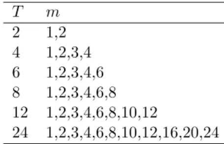
We consider the problem of dynamic allocation of a scare resource, which in our case is donor– funding, to patients in different health states over a finite horizon. The planning horizon is divided intoT periods, with time indexing done in the reverse order, i.e., periodT is the first period, followed byT-1,T-2,..., and so on. At the start of any periodt, we assume that there are
n1t patients in the less–severe health state, labeled ‘state 1’ and n2t patients in a more–severe health state, labeled ‘state 2’. In the malnutrition context, state 1 could be thought of as representing children suffering from moderate acute malnutrition and state 2 to be representing severe acute malnutrition. While it is possible that there could be more than two health states depending on the disease, we believe that the two–state model captures the key trade–offs inherent in resource allocation problems faced by public health managers, while keeping the model tractable for computational purposes. Before we get into the dynamics concerning n1t
and n2t, let us first explain the distinguishing factors between health states 1 and 2.
The two states differ from one another along three key dimensions: 1. how the health state changes in response to “non–treatment” in any given period. 2. the per–period costs associated with being in state i, i= 1,2, and 3. the terminal cost. Let us first discuss the evolution of the patients’ health states in the absence of treatment. In any given period, when treatment is not provided, we assume that α11 fraction of the patients in state 1 will continue to remain in state 1, while the remainingα12= 1−α11fraction deteriorate to state 2. In case of state 2, in the absence of treatment, we assume that α22 fraction of the patients will continue to remain in state 2, while the remaining α2E=1−α22 fraction exit the system. Patients could exit the system for a variety of reasons, e.g., death, defaulting, loss of confidence in the program etc. In our analysis, we do not distinguish between the different reasons (since in practice it is often difficult to ascertain the exact reason) and assume that for every patient who exits the system in periodt, we incur a fixed penalty oflEt . In the traditional Operations Management literature,
![Table 2.2: Average relative % cost difference as a function of CR for N =6, U ∼[70,130] demand distribution and 100% funding level](https://thumb-us.123doks.com/thumbv2/123dok_us/7973150.2116486/33.918.246.703.704.831/table-average-relative-difference-function-demand-distribution-funding.webp)