International Journal of Innovative Computing 6(2) 25-32
International Journal
of
Innovative Computing
Journal Homepage: http://se.fsksm.utm.my/ijic/index.php/ijicRegression Models with Multiobjective GA for EDM
Parameters Optimization
Yusliza Yusoff, Azlan Mohd Zain
Department of Computer ScienceFaculty of Computing 81310 UTM Skudai, Johor Bahru [email protected], [email protected]
Habibollah Haron, Roselina Sallehudin
Department of Computer ScienceFaculty of Computing 81310 UTM Skudai, Johor Bahru [email protected], [email protected]
Abstract—Over recent years, regression model is a well known modeling technique used to model the real world application. This paper conducted computational experimental study using two types of regression models; second order polynomial regression (SOP) and multiple linear regression in optimizing machining process parameters of cobalt-bonded tungsten carbide (WC/Co) electrical discharge machining (EDM). Multiobjective genetic algorithm (MOGA) is widely known in optimization researches. Therefore, combination of conventional modeling (regression) and modern optimization (MOGA) techniques, MLR-MOGA and SOP-MOGA are examined to observe the capability of these two techniques in maximizing removal rate (MRR) and minimizing surface roughness (Ra). Four parameters are considered to create correlation with the machining performances. The best removal rate and surface roughness values are obtained from MLR-MOGA; 168.212 mg/min and 0.693 µm respectively. Nevertheless, SOP-MOGA produced viable results. The results of MLR-MOGA and SOP-MOGA benefits the machine operators or engineers when various combination of machining parameters can be selected based on the desired requirements.
Keywords — Machining, Genetic Algorithm, Regression, Multiobjective
I.INTRODUCTION
Machining can be divided into two categories; (i) modern machining and (ii) traditional machining. Known as the earliest modern machining, EDM is a well established machining option used to remove material through the action of electrical discharge in fast mode and high current density. One of EDM research interests is optimizing the process parameters as highlighted by Ho and Newman [1].
Machining models are developed to represent the connection between input (machining parameters) and output (machining performances) variables. There are many
modeling techniques in machining optimization such as fuzzy logic [2], support vector machine [3], artificial neural network (ANN) [4] and many more.
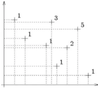
New soft computing techniques are developed to assist in searching optimal solutions such as genetic algorithm (GA) [5], Levi flight algorithm [6], glowworm swarm optimization [7], firefly algorithm [8] and many more. GA is one of the most popular techniques in the machining optimization area as studied by Yusup et al. [9]. Multi objective GA is an optimization technique that is enhanced from single objective genetic algorithm to support the multi objectives problems. One of the pioneer in multi objective GA; MOGA [10] implemented a rank based fitness assignment and niche-formation methods to encourage the search toward Pareto front in the optimization algorithm. According to the theory of Fonseca and Fleming [10], all non dominated individuals are assign rank 1 as in Figure 1.
Fig. 1. Multiobjective ranking
of three parameters, (i) depth of cut, (ii) feed rate and (iii) cutting speed. The authors used MOGA technique to obtain the process parameters that can be applied in various cases of milling optimization process. Mahdavinejad [14] optimized the turning parameters of steel using MOGA and multi-objective harmony search (HS) algorithm Geem et al. [15] to optimize removal rate and surface roughness. Sultana and Dhar [16] used response surface methodology (RSM) to develop machining model and MOGA to optimize the process parameters of turning AISI-4320 steel by uncoated carbide insert. The process parameters considered are cutting speed, feed rate, pressure and flow rate of high pressure and the objectives considered are cutting temperature, chip reduction co-efficient and surface roughness. Venkataraman [17] maximized removal rate and minimized electrode wear rate (EWR) for EDM. Five parameters considered are open voltage, pulse on time, duty cycle and pressure of flushing fluid. Polynomial model and multi objective genetic algorithm are used to optimize the machining process.
Kanagarajan et al. [18] employed second order polynomial regression and non dominated sorting genetic algorithm (NSGA-II) to optimize the machining parameters of WC/Co EDM. Yusoff et al. [19] then applied the model developed by Kanagarajan et al. using both; single (SoGA) and multi objective optimization techniques (MOGA and NSGA-II). It is found that SoGA produced the lowest surface roughness value and the results obtained from MOGA are viable compared to NSGA-II. In conjunction with the experimental conducted by Yusoff et al. [19], this study investigated and compared the efficiencies of regression modeling techniques in optimizing of WC/Co EDM parameters using MOGA. Basically, this study is conducted to observe the performances of two different regression models when integrated with MOGA in machining optimization.
II.RESEARCH METHODOLOGY
Essentially, this study employed four consecutive ways in obtaining the final optimal solutions. The steps involved; collection of experimental data, modeling, optimization and results analysis. Second order polynomial (SOP) and multiple linear regression (MLR) are used to obtain the machining models. Multiobjective GA (MOGA) is used to optimize the parameters. Using computational and soft computing techniques in obtaining optimal solutions can reduce the machining trials that involved extreme cost, time and attempt in searching the best parameters.
The parameters considered are electrode rotation (R), current (I), pulse on time (T) and dielectric flushing pressure
(P). Removal rate (MRR) and surface roughness (Ra) are the machining objectives or also known as the machining performances.
To correlate the machining inputs (machining parameters) and outputs (machining performances), two types of regression models are applied. Second order polynomial regression (SOP) developed by Kanagarajan et al. and multiple linear regression (MLR) which is developed using
SPSS software. The models are then integrated in the optimization tool, MOGA using Matlab software to obtain the optimal solutions.
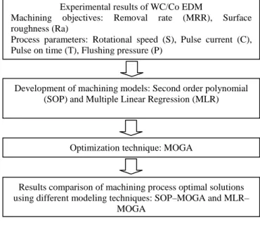
Finally the results of these two techniques are compared. The flow of this study is summarized as shown in Figure 2 and further details in next sub-sub sections.
Fig. 2. Research flow
A.Experimental
The experimental results by Kanagarajan et al. [18] are used in this study. The authors used a machine of Electronica die sinking EDM (M100 model, Electronica, India) with a transistor switched power supply. Density for WC is 15.7 g/cc and CO is 13.55 g/cc. The grain sizes are 6µm and 3µm respectively. The machining conditions of this study are shown in Table I.
TABLE I. MACHINING CONDITIONS
Condition Descriptions
Electrode Material: copper (electrolytic grade) Size: cylindrical with a diameter of 13 mm Workpiece Material: tungsten carbide 70% WC/ 30% Co
Size: cylindrical rod of diameter 13 mm Dielectric fluid: kerosene
Flushing Jet flushing
Flushing pressure: 0.5-1.5 Rotational speed
Discharge current Pulse on time
250, 500, 1000 rpm 5, 10, 15 A 200, 500, 1000
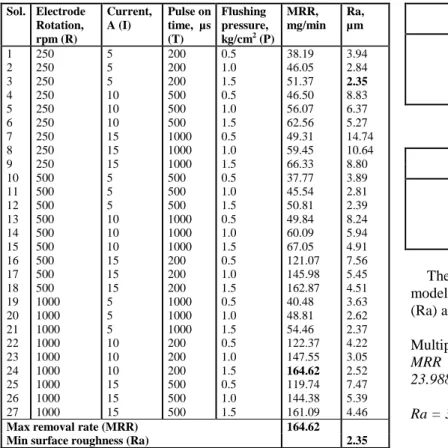
The experimental results of WC/Co EDM as shown in Table II are based on L27 orthogonal array technique covering full range of current setting with pulse on time settings.
Experimental results of WC/Co EDM
Machining objectives: Removal rate (MRR), Surface roughness (Ra)
Process parameters: Rotational speed (S), Pulse current (C), Pulse on time (T), Flushing pressure (P)
Development of machining models: Second order polynomial (SOP) and Multiple Linear Regression (MLR)
Optimization technique: MOGA
Results comparison of machining process optimal solutions using different modeling techniques: SOP–MOGA and MLR–
TABLE II. EXPERIMENTAL RESULTS OF WC/CO EDM
Sol. Electrode Rotation, rpm (R) Current, A (I) Pulse on time, µs (T) Flushing pressure, kg/cm2 (P)
MRR, mg/min Ra, µm 1 2 3 4 5 6 7 8 9 10 11 12 13 14 15 16 17 18 19 20 21 22 23 24 25 26 27 250 250 250 250 250 250 250 250 250 500 500 500 500 500 500 500 500 500 1000 1000 1000 1000 1000 1000 1000 1000 1000 5 5 5 10 10 10 15 15 15 5 5 5 10 10 10 15 15 15 5 5 5 10 10 10 15 15 15 200 200 200 500 500 500 1000 1000 1000 500 500 500 1000 1000 1000 200 200 200 1000 1000 1000 200 200 200 500 500 500 0.5 1.0 1.5 0.5 1.0 1.5 0.5 1.0 1.5 0.5 1.0 1.5 0.5 1.0 1.5 0.5 1.0 1.5 0.5 1.0 1.5 0.5 1.0 1.5 0.5 1.0 1.5 38.19 46.05 51.37 46.50 56.07 62.56 49.31 59.45 66.33 37.77 45.54 50.81 49.84 60.09 67.05 121.07 145.98 162.87 40.48 48.81 54.46 122.37 147.55 164.62 119.74 144.38 161.09 3.94 2.84 2.35 8.83 6.37 5.27 14.74 10.64 8.80 3.89 2.81 2.39 8.24 5.94 4.91 7.56 5.45 4.51 3.63 2.62 2.37 4.22 3.05 2.52 7.47 5.39 4.46
Max removal rate (MRR) 164.62
Min surface roughness (Ra) 2.35
B.Machining Models
From the machining results, two models are implemented; (i) second order polynomial model developed by Kanagarajan et al. [18] and (i) newly developed multiple linear regression model (MLR). The second order polynomial models for removal rate and surface roughness are shown in Equation 1 and Equation 2 for material removal rate (MRR) and surface roughness (Ra) respectively.
Second Order Polynomial Regression
MRR = -30.3660 + 0.1589R + 9.5259I - 0.1241T + 20.8585P - 0.0001R2 - 0.2318I2 + 0.0001T2 - 9.2131P2 - 0.0002RI - 0.0000RT + 0.0220RP + 1.9991IP - 0.0199TP
(1)
Ra = 4.2307 - 0.0116S + 0.5816C + 0.0099T - 4.7481P + 0.0000S2 + 0.0085C2 - 0.0000T2 + 2.1239P2 - 0.0002SC - 0.0000ST – 0.0020SP - 0.2462CP - 0.0018
(2)
Multiple linear regression equations of removal rate and surface roughness are based on the unstandardized coefficients values (B) of Tables III and IV.
TABLE III. COEFFICIENTS VALUES FOR MRR
Model Unstandardized Coefficients
B Std. Error
(Constant) R I T P -15.652 0.075 6.853 0.068 23.988 8.295 0.006 0.461 0.006 4.607
TABLE IV. COEFFICIENTS VALUES FOR RA
Model Unstandardized Coefficients
B Std. Error
(Constant) R I T P 3.734 -0.004 0.469 0.004 -2.771 0.815 0.001 0.045 0.001 0.453
The coefficients and constant for multiple linear regression models of material removal rate (MRR) and surface roughness (Ra) are given in Equation 3 and Equation 4.
Multiple Linear Regression
MRR = -15.652 + 0.075R + 6.853I- 0.68T + 23.988P
(3)
Ra = 3.734 - 0.004R + 0.469I + 0.004T - 2.771P (4)
C.Optimization
Based on NSGA-II introduced by Deb et al. [1], a multiobjective optimization tool, MOGA using Matlab is applied to obtain the optimal solutions. MOGA acts on individuals with better fitness value that can help to increase the diversity of the population even if they have a lower fitness value. It is very important to preserve the diversity of population for convergence to an optimal Pareto front by controlling the elite members of the algorithm.
The steps start with initialization by generating the random population. The next step is evaluation of the fitness of each chromosome using the multi objectives function (machining models). The algorithm parameters boundaries (Table V) are used to get solutions that are within the expected values.
TABLE V. ALGORITHM BOUNDARIES
Parameters Lower bound Upper bound
Rotational speed, rpm 250 1000
Pulse current, A Pulse on time, µs Flushing pressure, 5 200 0.5 15 1000 1.5
crowding distance is selected. Then crossover; new offspring is produce by combining subparts of selected chromosomes using recombination operator. Intermediate crossover is employed which creates two children from two parents. Mutation is carried out to introduce the deviation into chromosome to avoid premature convergence or segmentation. To improve the performance of genetic algorithm, elitist strategy is use to increase the speed of population domination. Using this strategy the best chromosomes are copied into the successive generation. Finally, termination of GA is when the stopping condition is satisfied; otherwise the circle will go to selection, crossover, mutation and so on for the next iteration. The flow repeats for successive generations. The final set of Pareto optimal solutions represents dominated solutions from the each generation and it is up to the decision maker to select a solution according to the selected objectives. The flow of MOGA optimization is illustrated in Figure 3.
Fig. 3. MOGA flow
The algorithm parameters for population, selection, mutation, crossover and generation are given in Table VI.
TABLE VI. ALGORITHM PARAMETERS
Parameters Value
Population size 100
Selection - Tournament Mutation - Uniform Crossover - Intermediate
4 0.25 0.9
Generation 1000
D.Results
MOGA is able to optimize more than one objective simultaneously resulted to time efficiency compared to single
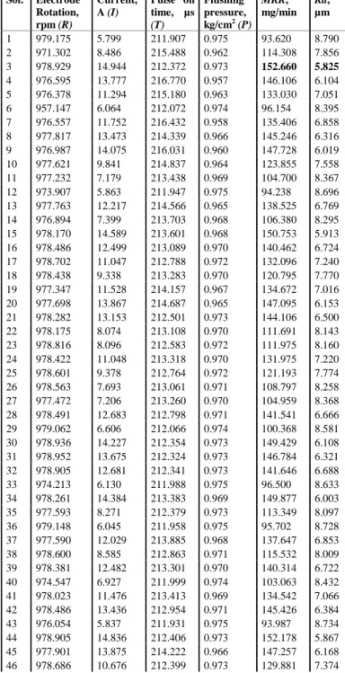
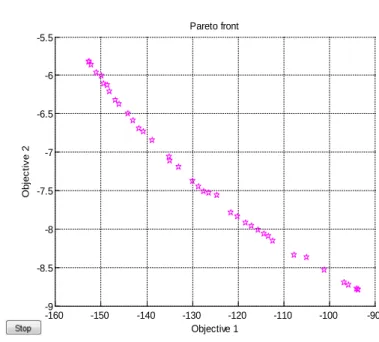
objective genetic algorithm. Optimizing machining process parameters using SOP-MOGA and MLR-MOGA are expected to give best set of estimation solutions. The maximum removal rate (MRR) , 152.660 mg/min and minimum surface roughness (Ra), 5.825µm values are obtained simultaneously using SOP-MOGA with R, I, T, P values are 978.929 rpm, 14.944 A, 212.372 µs, 0.973 kg/cm2 respectively. The same results of optimal solutions are generated twice as shown in Table VII. Figure 4 depicts the Pareto front of removal rate (MRR) and surface roughness (Ra) from SOP–MOGA optimization.
TABLE VII. SOP-MOGA OPTIMAL SOLUTIONS
Sol. Electrode Rotation, rpm (R)
Current, A (I)
Pulse on time, µs (T)
Flushing pressure, kg/cm2 (P)
MRR, mg/min
Ra, µm
1 979.175 5.799 211.907 0.975 93.620 8.790 2 971.302 8.486 215.488 0.962 114.308 7.856 3 978.929 14.944 212.372 0.973 152.660 5.825 4 976.595 13.777 216.770 0.957 146.106 6.104 5 976.378 11.294 215.180 0.963 133.030 7.051 6 957.147 6.064 212.072 0.974 96.154 8.395 7 976.557 11.752 216.432 0.958 135.406 6.858 8 977.817 13.473 214.339 0.966 145.246 6.316 9 976.987 14.075 216.031 0.960 147.728 6.019 10 977.621 9.841 214.837 0.964 123.855 7.558 11 977.232 7.179 213.438 0.969 104.700 8.367 12 973.907 5.863 211.947 0.975 94.238 8.696 13 977.763 12.217 214.566 0.965 138.525 6.769 14 976.894 7.399 213.703 0.968 106.380 8.295 15 978.170 14.589 213.601 0.968 150.753 5.913 16 978.486 12.499 213.089 0.970 140.462 6.724 17 978.702 11.047 212.788 0.972 132.096 7.240 18 978.438 9.338 213.283 0.970 120.795 7.770 19 977.347 11.528 214.157 0.967 134.672 7.016 20 977.698 13.867 214.687 0.965 147.095 6.153 21 978.282 13.153 212.501 0.973 144.106 6.500 22 978.175 8.074 213.108 0.970 111.691 8.143 23 978.816 8.096 212.583 0.972 111.975 8.160 24 978.422 11.048 213.318 0.970 131.975 7.220 25 978.601 9.378 212.764 0.972 121.193 7.774 26 978.563 7.693 213.061 0.971 108.797 8.258 27 977.472 7.206 213.260 0.970 104.959 8.368 28 978.491 12.683 212.798 0.971 141.541 6.666 29 979.062 6.606 212.066 0.974 100.368 8.581 30 978.936 14.227 212.354 0.973 149.429 6.108 31 978.952 13.675 212.324 0.973 146.784 6.321 32 978.905 12.681 212.341 0.973 141.646 6.688 33 974.213 6.130 211.988 0.975 96.500 8.633 34 978.261 14.384 213.383 0.969 149.877 6.003 35 977.593 8.271 212.379 0.973 113.349 8.097 36 979.148 6.045 211.958 0.975 95.702 8.728 37 977.590 12.029 213.885 0.968 137.647 6.853 38 978.600 8.585 212.863 0.971 115.532 8.009 39 978.381 12.482 213.301 0.970 140.314 6.722 40 974.547 6.927 211.999 0.974 103.063 8.432 41 978.023 11.476 213.413 0.969 134.542 7.066 42 978.486 13.436 212.954 0.971 145.426 6.384 43 976.054 5.837 211.931 0.975 93.987 8.734 44 978.905 14.836 212.406 0.973 152.178 5.867 45 977.901 13.875 214.222 0.966 147.257 6.168 46 978.686 10.676 212.399 0.973 129.881 7.374
Tournament Selection to choose best individual as parent
Mutation to make random changes to individual
Crossover to combine individuals for next generation
Elitist Strategy
Stop
Generate initialization of population
-160 -150 -140 -130 -120 -110 -100 -90 -9
-8.5 -8 -7.5 -7 -6.5 -6 -5.5
Objective 1
O
bj
ec
ti
v
e 2
Pareto front
47 978.840 9.415 212.151 0.974 121.597 7.783 48 976.837 6.688 211.968 0.975 101.096 8.530 49 978.497 11.504 213.117 0.970 134.781 7.073 50 978.365 12.182 212.751 0.972 138.790 6.845 51 978.628 11.941 212.628 0.972 137.452 6.938 52 978.616 7.838 212.962 0.971 109.931 8.220 53 978.784 12.523 212.552 0.972 140.733 6.736 54 974.900 6.355 212.006 0.974 98.368 8.586 55 976.684 5.913 211.939 0.975 94.629 8.724 56 978.062 6.816 212.067 0.974 102.093 8.512 57 979.072 6.608 212.060 0.974 100.379 8.581 58 978.617 12.942 212.363 0.973 143.035 6.588 59 978.884 8.498 212.407 0.973 114.995 8.051 60 978.551 8.083 212.929 0.971 111.800 8.151 61 978.046 10.068 214.035 0.967 125.559 7.514 62 978.929 14.944 212.372 0.973 152.660 5.825 63 977.966 9.230 213.401 0.969 120.015 7.792 64 978.484 11.177 212.622 0.972 132.936 7.198 65 978.445 9.116 212.253 0.974 119.492 7.865 66 978.565 7.480 212.110 0.974 107.366 8.341 67 978.905 13.519 212.416 0.973 145.982 6.377 68 978.814 9.570 212.552 0.972 122.563 7.724 69 978.044 8.398 212.401 0.973 114.277 8.067 70 978.681 10.150 212.734 0.972 126.409 7.535 71 978.467 14.092 213.166 0.970 148.576 6.127 72 978.757 10.465 212.356 0.973 128.549 7.445 73 977.361 6.489 211.955 0.975 99.454 8.589 74 977.621 9.921 213.727 0.968 124.660 7.562 75 978.820 14.594 212.407 0.973 151.104 5.961 76 978.961 9.212 212.308 0.973 120.142 7.843 77 978.626 12.152 212.842 0.971 138.600 6.857 78 978.516 11.559 213.017 0.971 135.124 7.057 79 978.156 12.835 213.629 0.968 142.136 6.581 80 979.144 6.170 211.967 0.975 96.760 8.696 81 978.575 8.137 212.204 0.974 112.374 8.155 82 978.882 9.581 212.429 0.973 122.666 7.725 83 978.695 8.967 212.636 0.972 118.340 7.903 84 978.917 13.949 212.392 0.973 148.099 6.214 85 978.955 10.298 212.208 0.974 127.498 7.507 86 974.490 5.856 211.942 0.975 94.170 8.706 87 978.822 8.775 212.538 0.972 116.985 7.965 88 979.170 5.844 211.917 0.975 94.000 8.779 89 978.967 8.953 212.177 0.974 118.346 7.924 90 978.405 12.807 213.054 0.971 142.138 6.612 91 977.577 9.775 212.684 0.972 123.944 7.637 92 979.108 7.507 212.034 0.974 107.588 8.343 93 976.845 6.177 212.209 0.974 96.801 8.654 94 978.497 11.504 213.117 0.970 134.781 7.073 95 976.054 5.837 211.931 0.975 93.987 8.734 96 974.213 6.130 211.988 0.975 96.500 8.633 97 979.175 5.799 211.907 0.975 93.620 8.790 98 978.551 8.083 212.929 0.971 111.800 8.151 99 978.960 11.485 212.305 0.973 134.870 7.110 100 979.121 7.692 212.009 0.955 108.334 8.200
Max removal rate (MRR) 152.660
Min surface roughness (Ra) 5.825
Fig. 4. Pareto front of MRR (objective 1) and Ra (objective 2) using SOP-MOGA
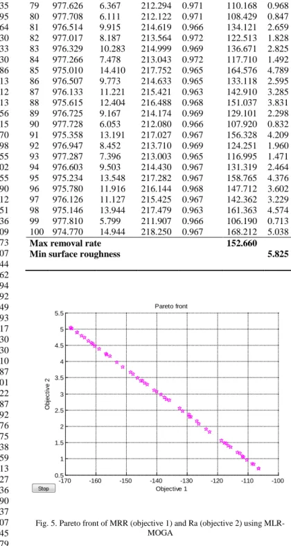
The optimal solutions of MLR-MOGA for removal rate and surface roughness are obtained separately as indicated in Table VIII. Maximum removal rate (MRR) is attained from the first set of solutions. While the optimal solutions for surface roughness is obtained from the second set of solutions. The maximum value for removal rate is 168.212mg/min with combination of process parameters R = 974.770 rpm, I = 14.944 A, T = 218.250 µs and P = 0.967 kg/cm2. Meanwhile, the minimum surface roughness (Ra) is 0.693 µm and the process parameters are R = 977.810 rpm, I = 5.799 A, T = 211.907 µs and P = 0.973 kg/cm2. The Pareto front plots of removal rate (MRR) and surface roughness (Ra) using MLR-MOGA is shown in Figure 5.
TABLE VIII. MLR-MOGA OPTIMAL SOLUTIONS
Electrode Rotation, rpm (R)
Current, A (I)
Pulse on time, µs (T)
Flushing pressure, kg/cm2 (P)
MRR,
mg/min Ra, µm
1 974.770 14.944 218.250 0.967 168.212 5.038
2 977.810 5.799 211.907 0.973 106.366 0.693
3 977.546 6.595 212.461 0.931 110.743 1.187
4 977.620 6.382 212.341 0.949 109.726 1.037
5 976.302 10.391 215.067 0.946 136.852 2.940
6 977.718 6.059 212.102 0.953 107.639 0.872
7 975.848 12.221 216.048 0.953 149.464 3.785
8 976.860 9.275 213.910 0.951 129.437 2.398
9 976.924 8.583 213.764 0.946 124.585 2.086
10 975.560 12.651 216.603 0.960 152.523 3.970
11 977.503 6.734 212.549 0.964 112.471 1.162
15 975.560 13.215 216.603 0.960 156.389 4.235
16 977.230 7.635 213.123 0.961 118.528 1.595
17 976.805 8.834 214.007 0.961 126.634 2.164
18 975.426 13.232 216.886 0.966 156.605 4.230 19 975.928 11.525 215.878 0.962 144.919 3.433
20 977.322 7.252 212.927 0.956 115.787 1.430
21 976.711 9.113 214.205 0.964 128.619 2.286
22 977.810 5.799 211.907 0.966 106.190 0.713
23 975.837 11.888 216.055 0.959 147.325 3.612 24 976.222 10.642 215.247 0.963 138.948 3.013
25 976.488 9.873 214.708 0.961 133.685 2.656
26 976.320 10.358 215.028 0.950 136.716 2.915
27 976.683 9.240 214.270 0.956 129.274 2.370
28 976.395 10.169 214.902 0.960 135.672 2.798 29 975.050 14.124 217.676 0.965 162.607 4.655
30 976.596 9.548 214.449 0.961 131.485 2.502
31 975.785 12.409 216.152 0.960 150.901 3.855 32 974.878 14.629 218.026 0.966 166.075 4.890 33 975.837 11.888 216.055 0.959 147.325 3.612
34 976.544 9.664 214.561 0.963 132.320 2.551
35 975.866 11.706 215.967 0.956 146.009 3.536 36 975.910 11.515 215.872 0.969 145.022 3.409
37 977.546 6.598 212.458 0.973 111.767 1.073
38 974.793 14.879 218.203 0.967 167.771 5.007 39 975.366 13.457 217.020 0.963 158.060 4.344
40 977.220 7.617 213.140 0.970 118.615 1.562
41 976.283 10.402 215.098 0.965 137.369 2.894
42 976.599 9.531 214.474 0.961 131.386 2.492
43 977.363 7.162 212.845 0.969 115.509 1.349
44 977.810 5.799 211.907 0.973 106.366 0.693
45 976.960 8.360 213.684 0.969 123.621 1.917
46 975.129 14.280 217.506 0.964 163.667 4.730 47 975.272 13.436 217.207 0.965 157.942 4.330
48 976.510 9.788 214.632 0.962 133.155 2.610
49 977.058 8.088 213.481 0.969 121.787 1.787
50 977.470 6.846 212.621 0.969 113.356 1.201
51 976.180 10.888 215.317 0.965 140.689 3.122 52 976.188 11.018 215.305 0.964 141.551 3.187
53 977.308 7.357 212.988 0.951 116.400 1.492
54 975.164 13.758 217.428 0.967 160.185 4.476 55 976.348 10.566 214.973 0.963 138.469 2.975 56 976.335 10.280 214.993 0.964 136.539 2.838 57 975.462 13.059 216.814 0.962 155.322 4.159 58 976.118 10.891 215.439 0.970 140.798 3.113
59 977.170 7.734 213.244 0.966 119.320 1.627
60 975.866 11.706 215.967 0.956 146.009 3.536 61 974.878 14.629 218.026 0.966 166.075 4.890
62 977.620 6.382 212.341 0.949 109.726 1.037
63 976.962 8.353 213.677 0.971 123.633 1.907
64 975.168 13.883 217.433 0.963 160.945 4.545
65 976.842 8.714 213.929 0.971 126.070 2.079
66 975.564 12.952 216.610 0.962 154.611 4.108
67 977.570 6.536 212.411 0.972 111.329 1.046
68 975.966 11.469 215.761 0.963 144.571 3.404
69 977.031 8.169 213.537 0.968 122.309 1.828
70 975.527 12.692 216.676 0.967 152.954 3.972 71 975.179 14.081 217.401 0.964 162.323 4.635
72 977.345 7.272 212.880 0.972 116.316 1.394
73 975.855 11.680 215.986 0.969 146.139 3.487 74 975.743 12.036 216.223 0.968 148.530 3.658 75 976.235 10.767 215.207 0.966 139.878 3.064 76 975.977 11.329 215.739 0.968 143.727 3.325 77 975.968 11.342 215.752 0.969 143.850 3.326 78 975.942 11.468 215.825 0.964 144.591 3.399
79 977.626 6.367 212.294 0.971 110.168 0.968
80 977.708 6.111 212.122 0.971 108.429 0.847
81 976.514 9.915 214.619 0.966 134.121 2.659
82 977.017 8.187 213.564 0.972 122.513 1.828
83 976.329 10.283 214.999 0.969 136.671 2.825
84 977.266 7.478 213.043 0.972 117.710 1.492
85 975.010 14.410 217.752 0.965 164.576 4.789
86 976.507 9.773 214.633 0.965 133.118 2.595
87 976.133 11.221 215.421 0.963 142.910 3.285 88 975.615 12.404 216.488 0.968 151.037 3.831
89 976.725 9.167 214.174 0.969 129.101 2.298
90 977.728 6.053 212.080 0.966 107.920 0.832
91 975.358 13.191 217.027 0.967 156.328 4.209
92 976.947 8.452 213.710 0.969 124.251 1.960
93 977.287 7.396 213.003 0.965 116.995 1.471
94 976.603 9.503 214.430 0.967 131.319 2.464
95 975.234 13.548 217.282 0.967 158.765 4.376 96 975.780 11.916 216.144 0.968 147.712 3.602 97 976.126 11.127 215.425 0.967 142.362 3.229 98 975.146 13.944 217.479 0.963 161.363 4.574
99 977.810 5.799 211.907 0.966 106.190 0.713
100 974.770 14.944 218.250 0.967 168.212 5.038
Max removal rate 152.660
Min surface roughness 5.825
-170 -160 -150 -140 -130 -120 -110 -100
0.5 1 1.5 2 2.5 3 3.5 4 4.5 5 5.5
Objective 1
O
bj
ec
ti
v
e 2
Pareto front
Fig. 5. Pareto front of MRR (objective 1) and Ra (objective 2) using MLR-MOGA
roughness value is shown in Table XI. The p values of SOP-MOGA and MLR-SOP-MOGA are 0.000517533 and 8.138E-05 respectively. The differences in surface roughness between experimental with SOP-MOGA and MLR-MOGA are also considered to be statistically significant. Though, p value of surface roughness is lower when using MLR-MOGA and provides better confidence level than SOP-MOGA.
TABLE IX. MLR-MOGA OPTIMAL SOLUTIONS
Model-Optimization
Electrode Rotation, rpm (R)
Current, A (I)
Pulse on time, µs (T)
Flushing pressure, kg/cm2 (P)
MRR, mg/min
Ra, µm
SOP-MOGA 978.929 14.944 212.372 0.973 152.660 5.825
MLR-MOGA 974.770 14.944 218.250 0.967 168.212 5.038 977.810 5.799 211.907 0.973 106.366 0.693
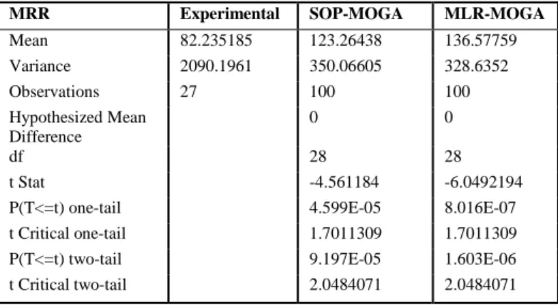
TABLE X. RESULT COMPARISON OF MRR
MRR Experimental SOP-MOGA MLR-MOGA
Mean 82.235185 123.26438 136.57759
Variance 2090.1961 350.06605 328.6352
Observations 27 100 100
Hypothesized Mean Difference
0 0
df 28 28
t Stat -4.561184 -6.0492194
P(T<=t) one-tail 4.599E-05 8.016E-07
t Critical one-tail 1.7011309 1.7011309
P(T<=t) two-tail 9.197E-05 1.603E-06
t Critical two-tail 2.0484071 2.0484071
TABLE XI. RESULT COMPARISON OF RA
Ra Experimental SOP-MOGA MLR-MOGA
Mean 5.378148148 7.5066018 2.8434038
Variance 8.826023362 0.8302611 1.5969289
Observations 27 100 100
Hypothesized Mean Difference
0 0
df 27 29
t Stat -3.676352422 4.3288881
P(T<=t) one-tail 0.000517533 8.138E-05
t Critical one-tail 1.703288423 1.699127
P(T<=t) two-tail 0.001035066 0.0001628
t Critical two-tail 2.051830493 2.0452296
III.CONCLUSION
This paper presented comparative empirical results of using two types of regression models to integrate with multiobjective GA. Most researchers used second order polynomial regression [18, 20, 21, 22]. Lower level of regression model, multiple linear regression is used in this
study to compare the efficiency of these two techniques when integrating it with multi objective optimization, as in this case, MOGA is used. Generally, SOP-MOGA and MLR-MOGA are relevant in optimizing machining process parameters. The results proved that the best removal rate (MRR) and surface roughness (Ra) are obtained from MLR-MOGA. However, SOP-MOGA is able to generate possible maximum removal rate (MRR) and minimum surface roughness (Ra) values simultaneously from same solution without neglecting any of the objectives. From the results of MLR-MOGA, operators and engineers can choose either to maximize removal rate (MRR) or minimize surface roughness (Ra).
ACKNOWLEDGMENT
The authors highly appreciate the editors and reviewers for useful advices and positive comments. This work is partially sponsored by the Research Management Centre (RMC), Universiti Teknologi Malaysia (UTM) and Ministry of Higher Education Malaysia (MOHE) for funding throughout the Fundamental Research Grant Scheme (FRGS) vot. No. R.J130000.7828.4F721
REFERENCES
[1] K. H. Ho and S. T. Newman, "State of the art electrical discharge machining (EDM)," International Journal of Machine
Tools and Manufacture, vol. 43, pp. 1287-1300, 2003.
[2] M. R. H. Mohd Adnan, et al., "Fuzzy logic for modeling machining process: a review," Artificial Intelligence Review, vol. 43, pp. 345-379, 2013.
[3] A. M. Deris, et al., "Overview of support vector machine in modeling machining performances," Procedia Engineering, vol. 24, pp. 308-312, 2011.
[4] Y. Yusoff, et al., "Multi Objective Machining Estimation Model Using Orthogonal and Neural Network," Jurnal Teknologi, vol. Vol 78, 2016.
[5] A. M. Zain, et al., "An overview of GA technique for surface roughness optimization in milling process," 2008.
[6] A. F. Kamaruzaman, et al., "Levy flight algorithm for optimization problems-a literature review," in Applied
Mechanics and Materials, 2013, pp. 496-501.
[7] N. Zainal, et al., "Glowworm swarm optimization (GSO) for optimization of machining parameters," Journal of Intelligent
Manufacturing, pp. 1-8, 2014.
[8] N. F. Johari, et al., "Optimization of Surface Roughness in Turning Operation using Firefly Algorithm," in Applied
Mechanics and Materials, 2015, pp. 268-272.
[9] N. Yusup, et al., "Evolutionary techniques in optimizing machining parameters: Review and recent applications (2007-2011)," Expert Systems with Applications, vol. 39, pp. 9909-9927, 2012.
[10] C. M. Fonseca and P. J. Fleming, "Multiobjective genetic algorithms," in Genetic Algorithms for Control Systems
Engineering, IEE Colloquium on, 1993, pp. 6/1-6/5.
[11] K. Deb, et al., "A fast and elitist multiobjective genetic algorithm: NSGA-II," Evolutionary Computation, IEEE
Transactions on, vol. 6, pp. 182-197, 2002.
[12] Y. Yusoff, et al., "Overview of NSGA-II for optimizing machining process parameters," Procedia Engineering, vol. 15, pp. 3978-3983, 2011.
genetic algorithms," in Proceedings of the 3rd International
Conference on Manufacturing Engineering (ICMEN),
Chalkidiki, Greece, 2008.
[14] R. Mahdavinejad, "Optimizing of Turning parameters Using Multi-Objective Genetic Algorithm," vol. 118-120, ed, 2010, pp. 359-363.
[15] Z. W. Geem, et al., "A new heuristic optimization algorithm: Harmony search," Simulation, vol. 76, pp. 60-68, Feb 2001. [16] I. Sultana and N. R. Dhar, "GA based multi objective
optimization of the predicted models of cutting temperature, chip reduction co-efficient and surface roughness in turning AISI 4320 steel by uncoated carbide insert under HPC condition," 2010, pp. 161-167.
[17] R. Venkataraman, "Multi objective optimization of electro discharge machining of resin bonded silicon carbide," vol. 110-116, ed, 2012, pp. 1556-1560.
[18] D. Kanagarajan, et al., "Optimization of electrical discharge machining characteristics of WC/Co composites using non-dominated sorting genetic algorithm (NSGA-II)," International
Journal of Advanced Manufacturing Technology, vol. 36, pp.
1124-1132, 2008.
[19] Y. Yusoff, et al., "Experimental Study of Genetic Algorithm Optimization on WC/Co Material Machining " Journal of
Advanced Research in Materials Science vol. 21, pp. 14-26,
2016.
[20] S. Assarzadeh and M. Ghoreishi, "Statistical Modeling and Optimization of Process Parameters in Electro-Discharge Machining of Cobalt-Bonded Tungsten Carbide Composite (WC/6%Co)," Procedia CIRP, vol. 6, pp. 463-468, 2013/01/01 2013.
[21] C. Senthilkumar and G. Ganesan, "Electrical Discharge Surface Coating of EN38 Steel with WC/Ni Composite Electrode,"
Journal of Advanced Microscopy Research, vol. 10, pp.
202-207, 2015.