TECHNICAL UNIVERSITY OF CLUJ-NAPOCA
ACTA TECHNICA NAPOCENSIS
Series: Applied Mathematics, Mechanics, and Engineering Vol. 61, Issue IV, November, 2018
A MODEL FOR MEASURING THE POSITION OF A PENDULUM USING
OPTO-ELECTRONIC METHOD
Adrian MOCAN, Ioan CIASCAI
Abstract: We propose a theoretical model for measuring with precision the position of a pendulum. This measurement is useful for the monitoring of pendulum position used in dams to verify their structural integrity. This model will use only one photodetector array sensor to achieve a price effective implementation. The model consists in a linear array of photodetectors and a LED band placed in parallel with it having the pendulum wire running between them, perpendicular with their plane. The position of the pendulum will be computed by detecting its shadow on the photodetector array when a LED from the band is lit. Taking two of these measurements is possible to compute the position of the pendulum on both x and y axis. A third measurement is made to improve the accuracy. We will compute the pendulum position errors for this theoretical model so we can decide if an implementation is feasible.
Key words: Measure pendulum position, compute errors, optic method, dams.
1. INTRODUCTION
Monitoring structural integrity of dams is an activity of vital importance. A big part of this monitoring consists in measuring with high accuracy the position of a very long plumb line called pendulum. These pendulums are installed in dams and a certain change in their position may mean a modification in the structural integrity of the dam. An optical method to measure the position of the pendulum[6] is preferred because is not affecting the position of the wire.
We want to design a system to automatically read and relay further the position of a pendulum. This system will be built around a microcontroller[1] that uses optic sensors to read the pendulum position.
2. DESCRIPTION
2.1 Measurement Principle
The position of the pendulum can be found by taken two successive measurements in which a LED is lit and the position of the pendulum shadow for that LED is read from the
photodetector array. Knowing the positions for two LEDs and their shadows we can compute the position of the pendulum.
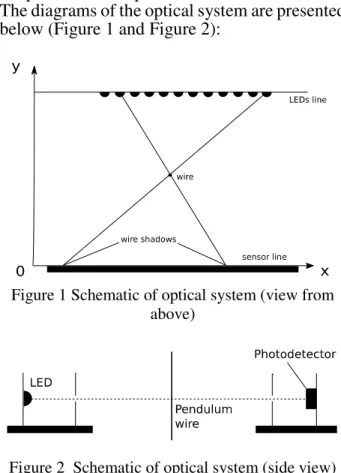
The diagrams of the optical system are presented below (Figure 1 and Figure 2):
Figure 1 Schematic of optical system (view from above)
To build the measurement system for the pendulum we considered a band of WS2812B LED type. On a band of WS1812B the LEDs can be controlled individually to the desired color and intensity [8].
For the part of light detection used to detect the shadow caused by the pendulum wire we considered TSL1412S sensor [2]. TSL1412S optical sensor consists in a linear array of photodetector pixels.
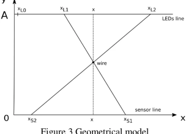
Let x and y be the coordinates for the pendulum. We take the x axis along with the photodetector array so that 0 coordinate is at pixel 0 and y axis in the plane of photodetector array and LED band (see Figure 3).
Figure 3 Geometrical model
Position of the pendulum (x and y) is computed from the similarity of the triangles (see Figure 3) through the following relations:
xL2 − xL1
xS1 − xS2 = − =xL2 −− xS2 (1)
We introduce some notation to simplify the calculation. Let it be dl = xL2 – xL1, ds = xS1 – xS2 and r = ds / (dl + ds). The physical meaning for r is revealed when r is expressed in terms of y and A. We can obtain from (1) that r represents the ratio of y to A.
With these substitutions, we can rewrite (1) into:
= − = − 2 (2)2 −
We can find y from the first equality by adding 1 to each side:
= ⋅ or = ⋅ (3)
We can find x from 1st and 3rd members of (1) after we collect x:
= ⋅ ⋅ or
= ⋅ xL2 + (1 − ) ⋅ xS2 (4)
Let us consider if x can be measured more precise if we were to use another measurement. At this point we can compute an approximation for x using the first two measurements as described above. We can use this value to light the closest LED to x and use this LED for the 3rd measurement (see Figure 4).
Figure 4 Geometrical model with the 3rd measurement
We could write then:
= − = − 3 (5)3 −
and compute x as:
= ⋅ ⋅ or
= ⋅ xL3 + (1 − ) ⋅ xS3 (6)
2.2 Error computation
In this paper we will focus on errors given by the geometry of the optical apparatus and ignore the errors caused by other sources of errors like the refraction of light in the LED and photodetector [3]. Thus the errors obtained here through calculation are the minimal values for the errors of pendulum positions that we can hope to achieve.
from errors of A and errors of r. In turn r is expressed by two independent measurements dl and ds so we can compute the error of r as composed of errors of dl and ds.
The error component due to A and r are given by the partial derivative of y (with respect to A and r) multiplied with the error of A and r. The partial derivative has the meaning of a factor that multiplies that error.
ˍ ˍ = part_y_r =
ˍ ˍ = | ˍ ˍ ⋅ |
ˍ ˍ = part_y_A =
ˍ ˍ = | ˍ ˍ ⋅ |
Because A and r are independent measurements we have:
err_y = err_y_A + err_y_r or
err_y = ( ⋅ dA) + ( ⋅ dr) (7)
We can see from (7) that to have small errors for y we need small errors for A and r (dA and dr).
Errors for r (dr) are computed below (using the same method):
part_r_ds = part_r_ds = ( )
err_r_ds = ∣∣part_r_ds ⋅ dds∣∣
ˍ ˍ = ˍ ˍ =
( )
ˍ ˍ = | ˍ ˍ ⋅ |
Because dl and ds are also independent we can write:
= ˍ ˍ + ˍ ˍ
= (( ⋅ ) ) + (( ⋅ ) ) or
dr =( ) ⋅ (dl ⋅ dds) + (ds ⋅ ddl) (8)
We can see from (8) that in order to have small errors for r we need to have dl and ds as large as possible. To accomplish that, we can have an algorithm that finds the position for LEDs by starting from each margin and
advancing toward the other margin until the shadow of the pendulum is cast on the photodetector array. This way we can ensure the largest value possible for both dl and ds.
If we turn our attention to x we can apply the same method here to compute the errors. Before we start we will introduce another source of errors that do not affect the errors on y axis. Let xL0 be the offset between the 0 coordinate on x axis and 0 coordinate on LEDs axis. In this case xL3 which is a value relative to 0 coordinate of photodetector will be expressed as a value on LEDs axis (relative to 0 coordinate of LED axis) as xL03, where xL3=xL0+xL03. We will use xL03 in further calculation. We can see that the axes offset does not affect at all any calculation for y. This is because xL0 is cancel out during calculation of dl, which is the only measurement potentially affected by xL0. Much in the same way xL0 does not affect the calculation for r in the first two measurements taken for x.
Now we will write the partial derivative with respect to xL0, xL3, xS3, r
part_x_xL03 = part_x_xL03 =
err_x_xL03 = ∣∣part_x_xL03 ⋅ dxL03∣∣
part_x_xS3 = part_x_xS3 = 1 −
err_x_xS3 = ∣∣part_x_xS3 ⋅ dxS3∣∣
part_x_r = part_x_r =
err_x_r = ∣∣part_x_r ⋅ dr∣∣
part_x_xL0 = part_x_xL0 =
err_x_xL0 = ∣∣part_x_xL0 ⋅ dxL0∣∣
where we took K=xL0+xL03-xS3.
We can consider at this point all the measurements independent so the error of x will be given by:
err_x = err_x_xL03 + err_x_xS3 + err_x_xL0 + err_x_r And replacing the computed partial derivative in the error component of each measurement we got:
err_x = ( ⋅ dxL03) + (1 − ) ⋅ dxS3 + ( ⋅ dxL0) + ( ⋅ dr)
Now we can prove the supposition that a 3rd measurement for x will reduce the errors. From (9) we see that the error for x is reduced if K takes small values, as this will reduce the contribution of dr. Because a small K is given by a measurement with xL03 and xS3 taken very close to x, this is exactly the case of the 3rd measurement taken for x.
Because the error of r appears in both expression for errors of x and y we will take some time to better analyze and estimate it. We can take from the datasheet of TSL1412S dds=63.5µm. The value of ddl could not be found from the documentation of the LED band so we took the experimental approach. We took several measurements of the distance between LEDs on the band and compute the standard deviation [5], so ddl = 190µm.
After computing some values of r it can be seen that if dl and ds are close to their maximum value (97mm) dr ≈ 6E-4. The value for dr increases if ds or dl is very small and increases very sharply if both ds and dl have very small values.
We consider now how the value of dr depends on the pendulum position (x and y) by taking into account the algorithm to find the appropriate LEDs described above. This algorithm finds the LEDs position so that for each pendulum position (x and y) the maximum dl and ds are found and then dr is computed for the given x and y. The graph of dr as a function of x and y (the pendulum position) can be seen in Figure 5:
Figure 5 3D representation of dr(x,y)
From figure 5 it can be seen that there is a central range for x and y where dr has small values and if the pendulum goes in the extremities of x, the values of dr will increase dramatically. We will use a contour graph (see
Figure 6) to take a better look at values for dr in the central region of x and y.
Figure 6 Contour graph of dr
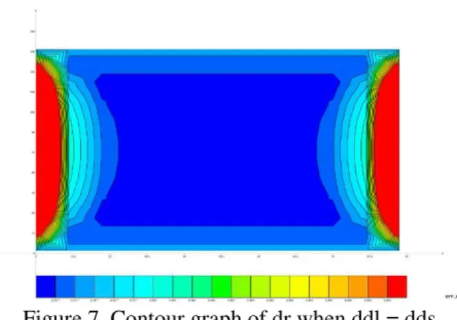
We can see that there is an asymmetry in the values of dr and we suppose that this asymmetry comes from the fact that ddl > dds. To test this supposition, we will take ddl equal to dds and redraw the graph (see Figure 7) of dr.
Figure 7 Contour graph of dr when ddl = dds
We can see from the new graph that we were right with the supposition, having closer error values for LED position to the error values for reading pixel position of photodetector will give a more uniform value for the dr in the central range of x and y.
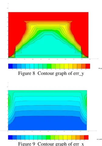
Now that we know the looks of dr(x,y) better, we can make the calculations for errors on x and y axes and represent them graphically. For the following graphs (Figure 8, 9, 10, 11), dark blue is 30 µm and red is 200 µm.
Figure 8 Contour graph of err_y
Figure 9 Contour graph of err_x
We want to see also how these graphs are affected when ddl = dds
Figure 10 Contour graph of err_y when ddl = dds
Figure 11 Contour graph of err_x when ddl = dds
3. CONCLUSION
From the analysis of the proposed theoretical model by using some concrete data from the LED band and photodetector TSL1412S we can conclude:
The positioning error of the LEDs on the band have the biggest contribution to the errors of x and y in the proposed model. Although the positioning error for the LEDs are only about 3 times as much as reading errors on the photodetector array, the increase of the errors in x and y is significant. Also, this relative small ratio between LED positioning errors and photodetector reading creates a big disturbance in the distribution of errors with regard to position of the pendulum. In this case the gradient of errors is big exactly in the middle of the reading area for the pendulum.
By using in calculation values for the LED positioning errors equal to the values of photodetector reading, the errors for pendulum position have smaller values and their distribution with pendulum position is very good in the important area of the middle x and y ranges.
One cost effective solution to lower the errors for the LED positioning to the levels of photodetector reading is to devise a calibration procedure where we can use the lower errors of photodetector reading to find the LED positions with a better accuracy and then store these positions in nonvolatile memory. Furthermore, this calibration procedure has the potential to eliminate some other type of errors (like refraction errors) that will affect the practical measurements.
We intend to design and build a measurement system based on the ideas exposed here. We will conduct research on how other sources of errors affect the position of the pendulum and how the errors can be reduced.
4. REFERENCES
[1] Ciascai I., Sisteme electronice dedicate cu microcontrolere AVR RISC. Editura Casa Cărţii de Ştiinţă, 2002.
[2] Ciascai I. and Ciascai L., “Acquire images with a sensor and a microcontroller,” EDN, no. EDN | SEPTEMBER 23, 2010, p. 48, 2010.
[3] Pop S., Ciascai I., Bande V., and Pitica D., “Modeling the light of LED’s for position detection with an optical sensor,” in 33rd International Spring Seminar on Electronics Technology, ISSE 2010, 2010, pp. 374–377. [4] Taylor J. R., An introduction to error
analysis: the study of uncertainties in physical measurements. University Science Books, 1997.
[5] Ross S. M., Introduction to Probability and Statistics for Engineers and Scientists. Elsevier Science, 2009.
[6] Pop S., Ciascai I., and Pitica D., “Statistical analysis of experimental data obtained from the optical pendulum,” in 2010 IEEE 16th International
Symposium for Design and
Technology in Electronic Packaging (SIITME), 2010, pp. 207–210.
[7] TAOS Inc., “TSL1412S 1536 × 1 LINEAR SENSOR ARRAY WITH HOLD,”
TAOS045F, Apr. 2007,
https://html.alldatasheet.com/html-pdf/203049/TAOS/TSL1412S/97/1/T SL1412S.html
[8] Worldsemi, “Intelligent control LED integrated light source”, WS2812B,
http://www.world-semi.com/DownLoadFile/108
UN MODEL PENTRU MĂSURAREA POZIȚIEI UNUI FIR CU PLUMB FOLOSIND O METODĂ OPTO-ELECTRONICĂ
Rezumat: Propunem un model teoretic pentru măsurarea cu precizie a unui fir cu plumb. Această măsurătoare este utilă la monitorizarea poziției unui fir cu plumb folosit la baraje pentru verificarea integrității structurale a lor. Modelul folosește doar un sigur fotodetector pentru o implementare cu cost redus. Modelul constă într-un array liniar de fotodetectori și o bandă de LED-uri plasată în paralel în timp ce firul cu plumb trece printre ele, perpendicular cu planul lor. Pozitia firului cu plumb va fi calculată detectând umbra lui pe array-ul de fotodetectori în momentul când un LED din bandă este aprins. Luând doua asemenea măsurători este posibil să calculăm poziția firului cu plumb atât pe axa x cât și pe axa y. O a treia măsurătoare se poate face pentru înbunătățirea acurateței. Vom calcula erorile de măsură pentru poziția firului cu plumb date de acest model pentru a decide cât de fezabilă este o implementare practică.
Adrian MOCAN, drd., Technical University of Cluj-Napoca, Department of Applied Electronics, 24-26 George Baritiu str. 400027 Cluj-Napoca, +40-723-873249, e-mail: [email protected].