TECHNICAL UNIVERSITY OF CLUJ-NAPOCA
ACTA TECHNICA NAPOCENSIS
Series: Applied Mathematics, Mechanics, and Engineering Vol. 61, Issue Special, September, 2018
AN INTEGRATED PLANNING AND SCHEDULING MODEL
FOR WIRING SYSTEMS ASSEMBLY
Radu-Constantin VLAD
Abstract: This paper presents a mixed integer programming model that could be used to schedule the assembly of wiring systems in the automotive industry. The assembly system consisted of several parallel independent workstations. The paper shows how the performance of a traditional integrated planning and scheduling model could be improved with the help of three additional constraints and priority coefficients in allocation of resources. The first constraint was a reformulation of the traditional material balance equation while the other two set the values of the planning variables when the demand for a particular period is higher than the average demand or the capacity of the assembly system. The priority allocation coefficients exploited the fact that workstations were identical.
Key words: integrated planning and scheduling, priority allocation coefficients, parallel independent workstations.
1. INTRODUCTION
1.1 The need for integration
Planning and scheduling have been two important instruments used in managing the activity of a system that either produced some goods or provided services. Planning focused more on balancing the demand of the customer with the rough-cut capacity of the system while scheduling specified, in detail, how resources should be used in order to meet the needs of the customer.
Obviously, the ultimate goal was to find the optimal schedule because it provided the framework that ensured that customer requests were efficiently satisfied. The quest for such a schedule has always been a challenging task because of the combinatorial nature of the scheduling problem.
Initially the task has been accomplished by considering a two-stage process. The first one, called planning, produced an aggregate plan that specified production targets for product families for every period of the planning horizon. The second stage aimed to formulate for every resource a detailed working plan based on the production targets set by planning.
In this way it was possible to obtain a schedule but, in most cases, it was not the optimum because planning did not take into account the sequence in which resources processed products or services. Despite the drawback, this approach has been frequently used because, on one hand, it was the only possibility at the time and, on the other, it was in line with management practice, as higher-level managers focused more on meeting customer demand while operational managers dealt with scheduling issues.
1.2 Characteristics of an integrated model An integrated planning and scheduling model (referred to as IPS model in this paper) should incorporate all general features of both planning and scheduling models. This means that an IPS model should take into account: 1. customer demand specified at certain moments in time;
2. resource capacity indicated for every period of the planning horizon;
3. moments when tasks or production of products would start or end;
4. set-up times required by resources to switch to a different product or task;
6. precedence constraints; 7. resource allocation rules.
From a modelling point of view, it could be concluded that an IPS model should contain both planning and scheduling variables. However, the integration of the two sets is not a trivial task because of the different scales of the time intervals on which the two sets of variables are defined.
Scheduling focuses mainly on fine details such as the sequencing of tasks over time. Resources are allocated in such models with the help of binary and/or integer variables. Since the computational effort is directly linked to the number of integer variables scheduling models were only developed for a short period of time. To this decision contributed also the fact that developing schedules for long intervals may not make sense given the number of factors that affect the activity of a production system.
In an IPS model the time horizon should be quite long in order to accommodate the requirements of a planning model. Too long a horizon and the corresponding model may not provide a solution in a reasonable amount of time or the solution may not be practical if the planning horizon is larger than the period during which customer demand is “frozen”. Perhaps this period should be the unit of measurement for the planning period for which the IPS model should be developed.
1.3Literature overview
Despite the difficulty in finding the optimal solution for a large IPS model the number of articles on this topic is quite high, so much so, that a literature overview has been performed in 2009 [7]. Maravelias and his colleague have suggested that IPS models should be classified based on modelling approaches and solution strategies [7]. The first criterion allowed the authors to identify three classes: detailed scheduling, relaxation and aggregations of scheduling and finally surrogate models [7]. With respect to solution strategies Maravelias and his colleague have classified contributions as: hierarchical, iterative and full-space [7].
Using the taxonomy introduced by Maravelias and Sung this paper could be related to contributions that aim to produce a detailed schedule using a full-space solution strategy.
Two comments could be made on the contributions of this class. First of all, the number of papers is quite small because the rapid increase of the computational time with the size of the problem has led researchers to finding alternative means to mathematical formulations. Secondly, models have a similar structure because they have to consider material balances, resource constraints generated by limited resource capacity and resource change-overs from a product to another. As a consequence of the latter, IPS models of this class differ through the way planning and scheduling variables are correlated and through the formulation of their constraints.
The most import factor related to correlation of planning and scheduling variables is time representation. Given the nature of the planning and the scheduling problems constraints have to be enforced of some points in time. Depending on how those points are defined the time grid may be fixed, with a constant number of intervals or with intervals of the same duration. Decisions related to time representation may lead to two classes of IPS models. The first one uses actually two time-grids: the planning grid that spans for weeks or months, and the scheduling grid where the time unit is usually the hour. In the models of the second class there is only one grid that has a time unit given by scheduling.
IPS models with two grids are used most often, for example Erdirik-Dogan and Grossmann have divided the planning intervals into slots. For each interval the number of slots was the same although of variable length [2]. An interesting solution has been employed by Gimenez, Henning and Maravelias while developing a network-based continuous-time representation for process scheduling. In this case the task allocated to a slot could “float” that is the beginning and the end of the task did not have to coincide with a time point [7]. The authors have used the continuous-time representation in order to reduce the number of decision variables that are generally generated by a two-grid approach.
resource allocation. For example, a common characteristic of the great majority of all IPS models is that they express the material balance in the form:
= + − ∀ (1)
where the inventory at the end of the current period (“t”) is given by the inventory at the end of the previous period, the production and the demand of period “t”.
A different formulation for the material balance constraint has been used by Joly, Moro and Pinto in planning and scheduling the activity of petroleum refineries [4]. The authors have determined the product level in a storage tank as the sum of the initial level and the amount that entered the tank, from the beginning until the current moment, minus the amount transferred from the tank up the current moment. This is a continuous process formulation to but it is in fact very similar to the one in (1).
1. PROBLEM DEFINITION
The model presented in this paper has been formulated to develop a schedule for a plant assembling wiring systems for the automotive industry. The assembly facility consisted of 4 lines, each having 6 workstations. A wiring system was completely produced by a workstation therefore stations were considered to be independent. Practically every workstation could have been used to produce any of the 8 product types assembled at the time. However, the company has decided to allocate some products to some assembly lines in order to ensure the efficiency of the processes supplying the workstations with materials and components. Table 1 indicates the allocation of products to lines used by the company.
Table 1
Product-line allocation table (PLAT1)
P1 P2 P3 P4 P5 P6 P7 P8
Line 1 X X X X
Line 2 X X
Line 3 X X
Line 4 X X
From a computational point of view the that fact that the lines were almost dedicated to the assembly of only two products was a major advantage. To test the capabilities of the proposed model an additional, slightly more complex, product-line allocation table has been considered. Its structure is presented in Table 2 (referred to hereafter as PLAT2).
Table 2 Modified product-line allocation table (PLAT2)
P1 P2 P3 P4 P5 P6 P7 P8
Line 1 X X X X
Line 2 X X X X Line 3 X X X X Line 4 X X X X
The activity of a workstation was based on a four-hour period. This meant that a workstation produced the same product during that period of time. Maintenance teams needed approximately 20 minutes to reconfigure a workstation if it had to switch to a new product type. Workstation operators also had a coffee break of the same duration after a four-hour period. Given these organisational issues the proposed model has been solved considering that the planning/scheduling horizon was formed of slots of 230 minutes.
The company also provided data on the time needed to assemble a wiring system, and, more importantly on the customer demand for each product type.
Unlike most IPS case studies, this time the demand was not specified at the end of each planning period but for every slot of the planning/scheduling horizon.
The company wanted to obtain a schedule for only a three-day period because its customers were not allowed to change orders with less than three days to the due date. To test the capability of the model the planning horizon has been extended to 7 days, that is 42 slots.
• case B – orders have been increased to ensure an overall system utilisation of 85%; • case C – total demand has been kept at the same level as in case B, but it has been redistributed by adding the demand for two slots for the product type with the largest orders; for this particular product type customer demand varied from zero in one slot to a “maximum” value in the next slot; the utilization per slot, considering all product types, varied from 30% to 100%;
• case D – the profile of the demand for the product type with the largest orders have been modified again so that periods of low demand would be followed by periods of high demand (several consecutive slots);
• case E – the entire demand for every product type has been concentrated in the last period of the planning/scheduling horizon.
2. MATHEMATICALFORMULATION
The formulation of the proposed model has been developed considering a single time grid that had its time points equally distributed at four-hour intervals.
Four indices have been used, namely: “i” – for assembly lines, “j” for workstations, “k” for product types and “t” for slots – periods of the planning/scheduling horizon.
The following parameters have been included:
• L - number of assembly lines;
• W - number of workstations per line; it
was assumed that all lines would have the same number of workstations;
• K - number of product types;
• T - number of slots in the planning
horizon;
• asmbTimek - duration of the assembly of a wiring system of product type “k”;
• dk,t - demand for product type “k” in slot “t”;
• asgni,k – indicates if product “k” could be assembled on line “i";
• wCapk – the maximum number of
products of type “k” that could be produced by a workstation;
• ulb – utilisation lower bound; it was set
to 85%;
• slot – duration of a period of the
planning/scheduling horizon; duration of a slot was set to 230 minutes;
• noStationsi – number of stations for each assembly line i;
• pri,j,k – priority coefficient; its value was calculated with the formula:
, , = − 1 ∙ ∙ + − 1 ∙ + (2)
As decision variables the following have been defined:
• Xi,j,k,t – binary variable equal to 1 if product type “k” has been allocated to workstation “j” from line “i" in slot “t”;
• Yi,j,k,t – integer variable that indicates the number of wiring systems of product type “k” to be produced at workstation “j” from line “i" in slot “t”;
• SFk,t – level of inventory of product type “k” at the end of the slot “t”;
• Zi,j,t – binary variable equal to 1 if in slot “t” at workstation “j” of line “i" there was a changeover.
The use of the Y variables is not mandatory but they have been included in the model because they could contribute to the reduction of the inventory costs. If only X variables were used then allocating a product to a workstation in a slot would result in the production of a number of wiring systems, equal to the capacity of the workstation. This number could be too large compared with the customer demand and therefore could lead to higher storage costs.
With the help of these parameters and variables it was possible to formulate the objective function as a sum of three terms (3).
The first term of this function was associated with transition costs. To avoid having a solution that was influenced by the salary of the worker performing the changeovers the first term of the objective function consisted only of the sum of the changeover variables.
The second element of the objective has been formulated as the sum of the inventory levels at the end of each slot.
identical, a fact that means that a product could be assembled on a number of workstations. Since any workstation could be used to assemble a particular harness it was thought that the model could be solved faster if the allocation of products to workstations would be made with the help of some priority coefficients. In line with these considerations the model tried to minimize the following:
, , + , + , , ∙ , , , (3)
The set of constraints was formed of the following:
, = , + , , , − , ∀ , ∀ (4)
, = , + , , , − , ∀ , ∀ (5)
, , , ≥ , −1∙ , ∀ , ∀ (6)
, , , ≥ , − , , , − , ∀ , ∀ (7)
, , , ≤ ∙ , , , ∀ , ∀ , ∀ , ∀ (8)
∙ , , , ≥ ∙ ∙ , , , ∀ , ∀ , ∀ , ∀ (9)
, , , ≤ 1 ∀ , ∀ , ∀ (10)
, , , ≤ , ∀ , ∀ (11)
, , , ≤ ∀ , ∀ (12)
, , , − , , , ≤ 1 + , , ∀ , ∀ , ∀ , ≥ 2 (13)
, , , − , , , ≤ , , ∀ , ∀ , ∀ , ≥ 2 (14)
It was assumed that the initial inventories for all product types were zero.
The set of constraints of the proposed model presents some characteristics that are generally found in most IPS models. The material balance is expressed by constraint (4). Capacity related restrictions are imposed with the help of
relations (8) and (9). The first one sets the upper bound for all Y variables to the value of the capacity of a workstation while the second one sets the lower bound for workstation utilisation to 85%.
The set of constraints restricts the values of the X variables through relations (10), (11) and (12). Constraint (10) states that a workstation j, from a particular line i, in any slot t, could be allocated to one product k, at the most. Constraint (11) ensures that products are allocated to workstations in line with operational restrictions. Constraint (12) limits the number of allocations that are made for line i in slot t to the number of workstations of line i.
The last two constraints, (13) and (14), set the values for Z variables. Based on the values of X variables in slot t and t-1 these two constraints set the value of the corresponding Z
variable to one whenever there was a changeover at workstation j of line i in slot t.
The set of restrictions contains also elements that are not usually present in common mathematical formulations. The first one, constraint (5), is another expression for the material balance. It is similar to the traditional one stated by constraint (4) but it sets of values for
SF variables taking into account only variables
Y and the demand from the previous slots [4]. Constraints (6) and (7) have been introduced to raise the values of variables Y whenever demand for slot t is higher than the average demand for the entire planning horizon or when the production for set for all periods before slot t
would not be enough to satisfy demand of slot t.
3. MODEL TESTING
Model’s capacity to produce a schedule for real, large systems has been tested with the help of five data sets. Case A data has been provided by an important wiring systems manufacturer. The other four sets contain data that has been chosen in accordance with two principles. The new customer demand data had to be close to the volumes used in case A, but it had to be distributed as differently as possible to provide challenging test cases.
GHz machine. The structure of the assembly system has led to a large model. It has to be mentioned that constraint (11) does improve the performance of the model because it eliminates a large number of search paths in the solution space. Table 2 shows that the assembly system could be thought of as being formed of two subsystems: one with 18 workstations that produces 4 products and the other one formed of 6 workstations that produce 4 products as well. The model still can be considered as a large model since the first of its submodels generates a number of approximately 3000 binary variables.
It is important to notice that by adopting input data in line with the allocation matrix presented in Table 2 the model has been used to solve a problem that is more difficult than that generated by the real system. Furthermore, the manufacturer has asked for a three-day schedule while all data sets have been developed for seven-day period.
The search for the optimum has been limited to 600s and the optimality tolerance was set to 0.01%. The model has been run several times to test the model in its initial formulation and later constraints (5), (6) and (7) have been removed successively to assess their impact on the model performance.
The following tables report the performance of the proposed model as the:
• duration of the interval in which a solution was found within the optimality tolerance; • total number of changeovers that have been made for all 24 workstations in all 42 slots; • total sum of inventories at the end of all slots, all workstations, all products.
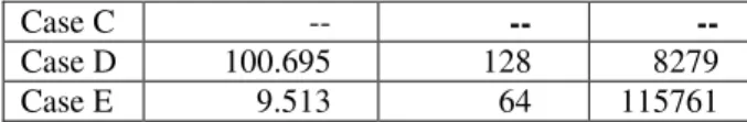
In its initial formulation the model produced the results presented in Table 3. For data set C the model failed to find a solution in 600s. The optimal solution was found for data set E in a small amount of time, perhaps due to the fact that all demand was concentrated in a single slot at the end of the planning/scheduling horizon.
Table 3
Results – initial model
time (CPUs) changeovers inventory
Case A 96.446 90 2450
Case B 152.902 109 3097
Case C -- -- --
Case D 100.695 128 8279
Case E 9.513 64 115761
In the next tests constraint (5) has been removed from the initial set of constraints. Results presented in Table 4 show that this time the model has failed to find a solution for two data sets that are characterized by high variability of the demand for product P1. Comparing results in Table 3 and 4 it is not possible to draw a clear conclusion on whether constraint (5) had a positive effect on model results. Table 4 shows that in case B the solution was found in a smaller amount of time but the number of changeovers was higher than in Table 3. Most of the data in Table 4 is worse than in Table 3 so it may be a good decision to keep constraint (5) in the model.
Table 4
Results – constraint (5) not considered
time (CPUs) changeovers inventory
Case A 153.12 91 2599
Case B 148.152 123 2881
Case C -- -- --
Case D -- -- --
Case E 8.857 66 116187
The experiments continued with the removal of constraint (6). This time a solution was found for all data sets (Table 5). Results from data sets D and E are quite similar with those from Table 3. In case B the time to solve the model and the number of changeovers were worse than those obtained through the initial formulation and perhaps are the best arguments to keep constraint (6). However, data from cases A and C do not support the conclusion.
Table 5
Results – constraint (6) not considered
time (CPUs) changeovers inventory
Case A 86.589 78 2439
Case B 201.765 124 2237
Case C 154.837 123 3564
Case D 105.241 122 8517
Case E 9.904 58 115779
Constraint (7) was considered next for removal from the initial model. Data in Table 6 show that in cases B and D this constraint may have helped reduce the time needed to solve the model. Cases A and C support the opposite conclusion as less time was needed to find the optimum.
Results – constraint (7) not considered
time (CPUs) changeovers inventory
Case A 71.436 71 2655
Case B 580.723 101 2449
Case C 169.944 123 3407
Case D -- --
Case E 9.56 64 115761
In the lasts tests it was the objective function that changed. The last term from its expression was removed so the model sought the optimum without priority coefficients. Table 7 shows that in the first four cases the model did not find the optimum in the 600s interval. However though, only in three cases the solution was worse off than in the initial formulation.
In case C although the model failed to find the optimum but it did find a “good” solution (as the gap reported by OPL was less than 1,31%). In the initial formulation no solution was found during the entire optimisation run.
For case E the performance of the model was better but similar to that of the initial formulation.
Table 7
Results – without priority coefficients
time (CPUs) changeovers inventory Case A 601.186 -
GAP - 2.91%
81 995
Case B 601.296 GAP - 3.78%
104 1194
Case C 601.736 GAP - 1.31%
124 2205
Case D 607.154 GAP - 1,26%
117 6320
Case E 5.67 56 109576
4. CONCLUSIONS
This paper presents a model that could be used to produce a schedule for a large system consisting of parallel identical and unrelated machines. It also tried to support the idea that mathematical models developed for large real systems could provide a good solution in a reasonable amount of time. To help reduce the time to solve the model three new constraints have been added to the classical formulation. With the same intent priority coefficients have been introduced in the objective function.
Tests have been conducted to determine if these changes do help the optimisation process. Results showed that for some data sets the proposed constraints have had a positive effect on
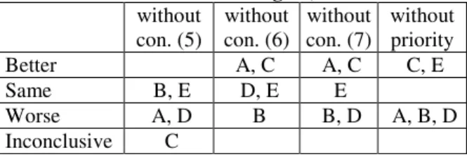
the final result while in other cases they did not. As data in Table 8 shows constraint (5) seems to contribute more than constraint (6) and (7) to the performance of the optimisation process. Since the tests carried out without constraint (5) did not produce better results than the initial formulation it has been concluded that it has to be included in the mathematical model.
The other two constraints, (6) and (7), have a different impact on the time to solve the model. For data sets A and C, the model needed more time to find the optimum while for data set E it was basically the same - only when the customer demand was relatively high and evenly distributed the two constraints reduced the time to find the best solution.
Priority coefficients did have a positive impact on the performance of the optimisation process. They seemed to be most beneficial when customer demand does not have a jigsaw profile.
Table 8
Summary of test results (compiled with data from tables 4 through 7)
without con. (5)
without con. (6)
without con. (7)
without priority
Better A, C A, C C, E
Same B, E D, E E
Worse A, D B B, D A, B, D Inconclusive C
The proposed model has been solved in conditions that were more demanding than those derived directly from the real system. Although heuristic approaches solve models of the same complexity faster, results presented in this paper show that traditional mathematical methods could still be used for solving large real-world problems.
5. ACKNOWLEDGMENTS
Students of the Management and Economical Engineering Department at the Technical University of Cluj-Napoca are gratefully thanked for making this material available. 6. REFERENCES
Engineering, Vol. 72, pp. 255-272, ISSN 0098-1354, (2015).
[2] Erdirik-Dogan, M., Grossmann, I.E., Simultaneous planning and scheduling of single-stage multi-product continuous plants with parallel lines, Computers & Chemical Engineering, Vol. 32, No. 11, pp. 2664-2683, ISSN 0098-1354, (2008).
[3] Gimenez, D.M., Henninng, G.P., Maravelias, C.T., A novel network-based continuous-time representation for process scheduling: Part I. Main concepts and mathematical formulation, Computers & Chemical Engineering, Vol. 33, pp. 1511-1528, ISSN 0098-1354, (2009).
[4] Joly, M., Moro, L.F.L., Pinto, J.M., Planning and Scheduling for Petroleum Refineries using Mathematical Programming, Brazilian Journal of Chemical Engineering, Vol. 19, No. 2, pp. 207-228, (2002).
[5] Kreipl, S., Pinedo, M., Planning and Scheduling in Supply Chains: An Overview of Issues in Practice, Production and Operations Management, Vol. 13, No. 1, pp. 77–92, ISSN 1059-1478, (2004).
[6] Leung, C.W., Wong, T.N., Mak, K.L., Fung, R.Y.K., Integrated process planning and scheduling by an agent-based ant colony optimization, Computers & Industrial Engineering, Vol. 59, No. 1, pp. 166-180, ISSN 0360-8352, (2010).
[7] Maravelias, C.T., Sung, C., Integration of production planning and scheduling: Overview,
challenges and opportunities, Computers & Chemical Engineering, Vol. 33, No. 12, pp. 1919-1930, ISSN 0098-1354, (2009).
[8] Merchan, A.F., Maravelias, C.T., Preprocessing and tightening methods for time-indexed MIP chemical production scheduling models, Computers & Chemical Engineering, Vol. 84, No. 4, pp. 516-535, ISSN 0098-1354, (2016).
[9] Sel, C., Bilgen, B., Bloemhof-Ruwaard, J.M., J.G.A.J. van der Vorst, Multi-bucket optimization for integrated planning and scheduling in the perishable dairy supply chain, Computers & Chemical Engineering, Vol. 77, pp. 59-73, ISSN 0098-1354, (2015). [10] Shah, N.K., Ierapetritou, M.G., Integrated production planning and scheduling optimization of multisite, multiproduct process industry, Computers & Chemical Engineering, Vol. 37, pp. 214-226, ISSN 0098-1354, (2012).
[11] Velez, S., Merchan A.F., Maravelias, C.T., On the solution of large-scale mixed integer programming scheduling models, Chemical Engineering Science, Vol. 136, pp. 139-157, ISSN 0009-2509, (2015).
[12] Wang, S., Liu, M., A branch and bound algorithm for single-machine production scheduling integrated with preventive maintenance planning, International Journal of Production Research, Vol. 51, No. 3, pp. 847-868, (2012).
UN MODEL INTEGRAT DE PLANIFICARE
ŞI PROGRAMARE A PRODUCŢIEI PENTRU ASAMBLAREA CABLAJELOR AUTO
Rezumat: Această lucrare prezintă un model de mixt de programare în numere întregi care poate fi folosit pentru a
programa asamblarea sistemelor de cablaje destinate industriei auto. Sistemul de asamblare a constat din mai multe
stații de lucru independente, paralele. Lucrarea arată cum poate fi îmbunătățită performanța unui model tradițional
integrat de planificare și programare cu ajutorul a trei constrângeri suplimentare și a coeficienților de prioritate în
alocarea resurselor. Prima constrângere suplimentară este o reformulare a ecuației tradiționale de echilibru a stocurilor
de produse în timp ce celelalte două stabilesc valorile variabilelor de decizie atunci când cererea pentru o anumită
perioadă este mai mare decât cererea medie sau decât capacitatea sistemului de asamblare. Coeficienții de prioritate au
exploatat faptul că stațiile de lucru au fost identice.