TECHNICALUNIVERSITY OF CLUJ-NAPOCA
ACTA TECHNICA NAPOCENSIS
Series: Applied Mathematics, Mechanics, and Engineering Vol. 61, Issue Special, September, 2018
GEOMETRICAL AND KINEMATICAL CONTROL FUNCTIONS FOR
A CARTESIAN ROBOT STRUCTURE
Claudiu SCHONSTEIN, Mihai STEOPAN, Razvan CURTA, Florin URSA
Abstract: Based on the idea of bringing more flexibility to a working process, the paper is dedicated to the presentation of geometry and kinematics equations for a Cartesian robot structure. The algorithms used in the mathematical modeling of mechanical robot structures, are used for establishing, on one hand of the homogeneous transformations in the direct geometry modeling, and on the other hand to determine the kinematics equations. The kinematic modeling of a mechanical system with n degrees of freedom, involves an impressive volume of computational or differential calculus. There are algorithms dedicated to this task developed in the literature. Will be established in analytical form, the direct equations for geometric and kinematic model using dedicated algorithms, for realize the kinematic control, namely the establishment of linear and angular speed/acceleration of every kinetic joint of robot and the tool central point.
Key words:mechanical systems, mathematical modeling, control functions, velocity, acceleration.
1. INTRODUCTION
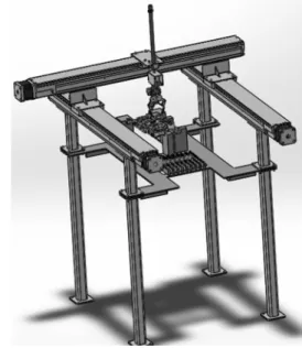
The robots are parts of the manufacturing systems, which are performing complex operations in order to achieve the imposed task. In keeping with the fact that the systems during operations are performing moving trajectories situated in the configuration space, or in the Cartesian space, it’s imposed a continuous control of every driving joint, in order to achieve a proper control of the kinematic parameters of the mechanical system, hence the purpose of the paper is to determine the kinematic equations for a Cartesian robot structure, presented in Fig. 1.
2. GEOMETRICAL MODELING OF THE
3TR ROBOT
In order to determine the kinematic control functions for the proposed 3TR robot structure, there must be determined first the geometry equations. Hence, using consecrated algorithms there can be determined the direct geometry equations, for the 3TR mechanical structure
proposed for implementation in an industrial process.
Fig. 1. The 3TR Cartesian robot structure
numerical and/or graphical form, on geometry, kinematics and dynamics of any mechanical structure of any type and complexity.
2.1 Direct Geometry Equations in Robotics
The Direct Geometry Equations (DGM equations) can be determined by applying the Matrix of Locating Algorithm, taking into account the minimum number of, geometric or mechanical restrictions. In concordance with [1], the situation matrix are defined as:
( ) ( )
1 0 0
1 1 0 0
1 ; 0
0 0 0 1 0 0 0 1
i
i i i i i i
i i i
R p R p
T T
−
− −
−
= =
. (1)
Similarly, for i =n+1, the locating matrices between the frames
{ }
n →{
n+1}
and{ }
0 →{
n+1}
are defined according to the following expressions:( ) ( ) ( ) ( )
( ) ( ) ( ) ( )
0 0 0 0
1 1
0 0 0 0
10 0 1
0 0 0 1
0 0 0 1
n
n n
n n
n n n n
n s a p T
n s a p T T T
+ +
+ +
=
= ⋅ =
(2)
In the expressions (2), p( )0 is a vector which defines the position of the last joint with reference system attached to base of the robot, and ( )0
1 n
n n
p + characterizes the relative position of the system attached to end effector besides the geometrical center of the last joint.
For i = 1→n, the situating matrices between two close related system
{
i−1}
→{ }
i are:(
;)
(
;)
(
1)
0 0 0 1
i
i i i i i i
i i
R k q q k
T∆ k q
⋅ ∆ − ∆ ⋅ ⋅
=
; (3)
[ ]
(
)
1
1 ;
i
i T Ti i T ki qi
−
− ∆
= ⋅ . (4)
According to [1]-[4], the rotation matrix between two neighboring reference frames is:
[ ]
{
(
) (
) (
)
}
1
; ; ; ; ;
i
i i i i i i i i i
i R R x q R y q R z q
−
= ⋅ ∆ ⋅ ∆ ⋅ ∆ (5)
( )0
(
)
1 1
1 1
i i i
i i i i i i
r p q k
− −
−
= + − ∆ ⋅ ⋅ . (6)
For i = 1→n, the position vector between
{ }
i and {i−1}with respect to{ }
0 fixed frame, respectively the position of joint{ }
i related to the same fixed frame is determined as:[ ]
0 1
1
1 i i 1
i i i i
p − = − R ⋅ −r − ; 1 1 i
i j j
j
p p − =
=
∑
. (7)The situation matrix, between { }0 →{ }i is:
[ ] [ ] [ ]
0
0 1
1 0 0 0 1
i
j i i
i j
j
R p T − T
=
= =
∏
. (8)and for the end-effector:
[ ] [ ]
0 0
1 1 0 0 0 1
n n n n
n s a p
T T T
+ +
= ⋅ =
. (9)
The orienting vector is defined [1]-[4] with the following identity:
(
A B C)
{
01[ ]
}
;(
A B C)
T nR α −β −γ = + R ψ = α β γ (10)
The DGM equations are included in the following generalized matrix:
0
T
x y z
T
x y z
p p p p
X
ψ α β γ
= =
. (11)
The Direct Geometrical Modeling (DGM), regardless of the algorithm used, aims to establish the geometry equations that will serve in determining the Direct Kinematic Model.
Fig. 2. The kinematic scheme of 3TR Robot
2.2 Direct Geometry Equations for 3TR
structure
For determining the DGM equations, it will be applied the Locating Matrix Algorithm. According to the first step, related to algorithm, it is represented in Fig. 2, the kinematic scheme of the robot in the initial configuration, when
1 l
0 O
( )0 4 O
2 q
1
q
a
s
n
0
z
0
x
0 y 2
l
( )0 1 O
3
q
1
z
1
x
1
y
3
l
4
l
2
z
2 x
2
y 3 z
3
x
3 y
4
q
5
l
4
z
4
x
4
all the generalized coordinates are initialized to
zero: ( )0
[
]
0; 1 4T
i
q i
θ = = = → .
According to the input data corresponding to DGM, the matrix of nominal geometry Mvn( )0 for 3TR robot type is given in Table 1.
Table 1 The matrix of nominal geometry for 3TR structure
E
le
m
en
t
Jo
in
t{
R
,T
}
[
1]
1@ pii− T =pi −pi− kTi
1
@ x
ii
p
− @pyii−1 @pzii−1 kix kiy kiz
1 T 0 0
1
l 1 0 0
2 T 0
2
l 0 0 1 0 3 T
3
l 0 0 0 0 1
4 R 0 0
4
l
− 0 0 1
5 - 0 0
5
l
− 1 0 0
As can be seen in the Fig. 2, the robot is included in to the class of mechanical olonomous systems, has four degrees of freedom, represented by the generalized coordinates as:
1 1
2 1
3 3
4 4
;
;
;
.
q Translation along x axis q Translation along y axis q Translation along z axis q Rotation around z axis
− ±
− ±
− ±
− ±
(12)
In keeping with Table 1, and Figure 2, there are highlighted the geometrical particularities for the 3TR serial robot, as following:
(
) (
)
(
) (
)
1 1 1 2 2 2
3 3 3 4 1 1
1; ; 0 ; 2; ; 0 ;
3; ; 0 ; 4; ; 1 .
i k x i k y
i k z i k z
= ≡ ∆ = = ≡ ∆ =
= ≡ ∆ = = ≡ ∆ =
(13)
According to (1), taking into account the fact that the first joint is translational joint, there is established:
[ ]
[ ] 00 1 3 1
1 1
1
1 0 0
0 1 0 0
0 0 1
0 0 0 1
0 0 0 1
q
R I p
T
l
≡
= =
(14)
For the second joint, on the basis of (3), (4) and (1), there is obtained:
[ ]
[ ] 11 2 3 21
2
2 2
1 0 0 0
0 1 0
0 0 1 0
0 0
0 1
1
0 0
0
R I p
T l q
≡
= =
+
(15)
To establish the homogenous transformation matrix, there is used expression (8), which leads to:
[ ]
[ ]1
2 0
0 2 3 2
2
2
1
1 0 0 0 1 0 0 0 1
0 0 0 1
0 0 0 1
R I
q l q
l p
T
≡
= ==
+
(16)
According to (4) there is obtained:
[ ]
[ ] 22 3
3
3 32
3
3
0
1 0 0
0 1 0 0
0
00 1 0 1
0 0 0 1
l
R I p
T
q
≡
= =
;(17)
On the basis of the same expression (8) in keeping with (16) and (17), there is obtained:
[ ]
[ ] 23 1 0
0 3 3 3
3
3 2
1
1 0 0
0 1 0
0 0 1
0 0 0 1
0 0 0 1
l q l
R I p
T q
l q
≡
= ==
+ +
+
(18)
For i =4, the situation matrices
{ }
4 →{ }
3 are:[ ]
[ ]4 4
3
3 4 43 4 4
4
4
cos sin 0
sin cos 0 0
0 0 1
0 0 0 1
0 1
0
0 0
q q
q
R p q
l T
−
= =
−
; (19)
which, in keeping with (18), according to (8) are leading to:
[ ]
24 4 3 1
0 4 4
4
2
1 4 3
cos sin 0
sin cos 0
0 0 1
0 0 0 1
q q l q
q q l q
l l q
T
−
=
+ +
− + (20)
For the coordinate system attached to the end effector, there is established :
[ ]
4
4 5
5
5
0 1 0 0
1 0 0 0
1 0 1
0 0 0 1
0 0 0 1
n s a p
T
l
= =
− −
(21)
and the homogenous transformation matrix, between {5}-{0} is :
[ ]
4 4 3 1
0 4 4
5
2 2
1 4 5 3
sin cos 0
cos sin 0
0 0 1
0 0 0 1
q q l q
q q l q
l l q
T
l
−
=
−
+ +
− − + (22)
In the expression, which characterizes the location matrix (20), are included the rotation matrix 0
[ ]
5 R and the vector position p5. The
[ ]
1
0 1
1 1
5
s c 0
c s 0
0 0 1
q q q q R
= −
−
(23)
3 1
5
1 4 5 3
2 2
l q l q l l l q p
=
+
−
+
− +
(24)
representing the resulting orientation matrix (23) and the position vector (24), between
{ }
5 →{ }
0 frames, both being included in the column vector of operational variables (11).According to [1], in order to establish the orientation angles, αx, βy, γz for determination of the values, there is used the trigonometric functionAtan 2, defined by:
(
)
[
]
{
}
[
]
{
}
[
]
{
}
[
]
{
}
; 0; 0 ;
/ 2 ; 0; 0
tan2 ;
; 0; 0 ;
/ 2 ; 0; 0
s c
s c x A s c
s c
s c
α α α
π α α α
α α
π α α α
π α α α
≥ >
+ > <
= =
+ < <
− + < ≥
(25)
Hence, in keeping with (25), results:
(
)
(
)
tan 2 ; tan2 0; 1
x A s x c x A
α = α α = − =π (26)
1
2
z π q
γ = + , and βy =0 (27) representing the orientation angles.
In keeping with (23)-(27), the column vector of operational coordinates, defined by (11), is:
( )
3 1
4 3
0
1
2 2
1 5
0
2
l q l q l l
q l
X q
π
π
−
=
+ +
+ −
+
(28)
The expression (28) characterizes the Direct Geometric Modeling of the robot type 3TR studied. The parameters included in (28) are expressing the position and orientation of the end effector with respect to the fixed reference system, attached to the base of the robot.
3. KINEMATICAL MODELLING OF
THE 3TR ROBOT STRUCTURE
In this paragraph will be established the operational kinematic parameters that express the movement of the end effector in Cartesian space. To define these parameters it is used the Iterative Algorithm. With this algorithm will be
defined the kinematic parameters with respect to the fixed reference frame, attached to the base. [5], [6].
3.1 The Iterative Algorithm for Direct Kinematical model
In applying the iterative algorithm according to [1],[3], for the first joint, i =1 it has to be assumed that absolute kinematic parameter values corresponding to the fixed base of the mechanical structure of the robot are:
{
0 0 0 0}
0 0, 0 0, v0 0, v0 0
ω = ω& = = & = (29)
For i = →1 n, there are determined the angular and linear velocities which are defining the absolute motion of each kinetic link using the expressions :
[ ] 0
0 0
1 i i
i i i R qi ki
ω = ω− + ∆ ⋅ ⋅& ⋅ (30)
(
)
(
)
0 0 0 0
1 1 1 1
i i i ii i i i
v = v− + ω− ×p − + − ∆ ⋅q& ⋅ k ; (31)
Similarly, for each i = →1 n, kinetic link of the robot, the corresponding angular and linear accelerations projected on the fixed reference system are defined as follows:
[ ] [ ]
{
0 0}
0 0 0
1 1 i i i i
i i i i qi R ki qi R ki
ω& = ω&− + ∆ ⋅ ω− ×& ⋅ ⋅ +&&⋅ ⋅ (32)
(
)
(
){
}
0 0 0 0 0
1 1 1 1 1 1
0 0 0
1 2
i i i ii i i ii
i i i i i i
v v p p
q k q k
ω ω ω
ω
− − − − − −
= + × + × × +
+ − ∆ ⋅ × ⋅ + ⋅
& & &
& &&
; (33)
In the second part of the iterative algorithm, are determined the kinematic parameters, which characterizing the movement in each i = →1 n
kinetic link relative to the { }i mobile frame as:
[ ]
[ ]
0 0 1
1 1
T i
i i i
i i R i i R i i qi ki
ω ω −ω
− −
= ⋅ = ⋅ + ∆ ⋅& ⋅ ; (34)
[ ]
[ ]
{
}
(
)
0 0 1 1 1
1 1 1
1
1
T i
i i i i
i i i i i i ii
i
i i i
v R v R v p
q k
ω
− − −
− − −
−
= ⋅ = ⋅ +⋅ × +
+ − ∆ ⋅& ⋅
.(35)
The expressions of angular and linear accelerations projected on the mobile reference system { }i , that characterizing the relative
movement of each i = →1 n link are defined by the following expressions:
[ ] [ ]
[ ]
{
}
0 0 1
1 1
1
1 1
i
i i
i i
i i i
i i i i
i
i i i i i i
R R
R q k q k
ω ω ω
ω
−
− −
−
− −
= ⋅ = ⋅ +
+∆ ⋅ ⋅ × ⋅ + ⋅
& & &
& &&
; (36)
[ ]
[ ]
{
}
(
)
(
)
0 1 1 1
1 1 1
1 1
1 1 1
1 1 1 1 2
i i
i i i i
i i i i i i ii
i i i i i i
i i ii i i i i i i
v R v R v p
p q k q k
ω
ω ω ω
− − −
− − −
− −
− − −
− − −
= ⋅ = ⋅ + × +
+ × × + −∆ ⋅ ⋅ × ⋅ + ⋅
& & & &
& &&
In the last step, the absolute motion of the final effector i =n is defined, taking into account the situation equations, respectively the absolute linear and angular velocities and accelerations (operating velocities and accelerations).
( )n0 ( )n0 T ( )n0 T T
n n
X& = v ω ; (38)
( )n0 ( )n0 T ( )n0 T T
n n
X&& = v& ω& . (39)
3.2 Direct kinematics equations for 3TR structure
In keeping with (13), according to (30)-(33), for the first joint of the robot, are determined:
[ ]
(
)
0
0 0 1
1
1 0 1 1 1 0 0 0
T
R q k
ω = ω + ∆ ⋅ ⋅& ⋅ = ; (40)
(
)
(
)
(
)
0 0 0 0
1 0 0 10 1 1 1 1 1 0 0
T
v = v + ω ×p + − ∆ ⋅q&⋅ k = q& (41)
{
}
[ ]
0 0 0 0 0
1 0 1 0 1 1 1 1
(3 1)
0
q k q k
ω ω ω
×
= + ∆ ⋅ × ⋅ + ⋅ =
& & & && ; (42)
(
)
(
)
{
}
(
)
0 0 0 0 0
1 0 0 10 0 0 10
0 0 0
1 1 1 1 1 1 1
1 2 0 0T
v v p p
q k q k q
ω ω ω
ω
= + × + × × +
+ − ∆ ⋅ × ⋅ + ⋅ =
& & &
& && &&
(43)
On the basis of the same (30)-(33) and (13), for the second joint, there is obtained:
[ ]
(
)
0
0 0 2
2
2 1 2 2 2 0 0 0
T
R k q
ω = ω + ∆ ⋅ ⋅ ⋅& = ;(44)
(
)
(
)
(
)
0 0 0 0
2 1 1 21 1 2 2 2 1 2 0
T
v = v + ω×p + − ∆ ⋅q& ⋅ k = q q& & (45)
[ ]
{
0 0[ ]}
[ ]
0 0 0 2 2
2 2
2 1 2 1 2 2 2 2
(3 1)
0
q R k q R k
ω ω ω
×
= +∆ ⋅ × ⋅ ⋅ + ⋅ ⋅ =
& & & && ;(46)
(
)
(
)
{
}
(
)
0 0 0 0 0
2 1 1 21 1 1 21
0 0 0
2 2 2 2 2 2 1 2
1 2 0T
v v p p
q k q k q q
ω ω ω
ω
= + × + × × +
+ − ∆ ⋅ × ⋅ + ⋅ =
& & &
& && && &&
(47)
The third driving joint of 3TR robot, is characterized by:
(
)
0 0 0
3 2 3 3 3 0 0 0
T
q k
ω = ω + ∆ ⋅& ⋅ = ; (48)
(
)
(
)
0 0 0 0
1
3 2 2 32 3 3 3 2
3
1 q
v
q
q
v ω p q k
= + × + − ∆ ⋅ ⋅ = & & & & ;(49) [ ]
{
0}
[ ]
0 0 0 3 0
3
3 2 3 2 3 3 3 3
(3 1)
0
q R k q k
ω ω ω
×
= + ∆ ⋅ × ⋅ ⋅ + ⋅ =
& & & && ;(50)
(
)
(
)
{
}
(
)
0 0 0 0 0
3 2 2 32 2 2 32
0 0 0
3 3 3 3 3 3 1 2 3
1 2 T
v v p p
q k k q q q q
ω ω ω
ω
= + × + × × +
+ − ∆ ⋅ ⋅ × ⋅ + ⋅ =
& & &
& && && && &&
(51)
The forth joint is characterized by the following kinematical parameters:
[ ]
(
)
0
0 0 3
3
4 3 3 3 3 0 0 4
T
q R k q
ω = ω + ∆ ⋅ ⋅ ⋅& & ;(52)
(
)
(
)
0 0 0
4 3 3 43 1 2 3
T
q q q
v = v + ω ×p = & & & ; (53)
(
)
0 0
4 3 0 0 4
T
q
ω& = ω& = && ; (54)
(
)
(
)
0 0 0 0 0
4 3 3 43 3 3 43 1 2 3
T
v& = v& + ω& ×p + ω × ω ×p = q q q&& && && (55) The expressions (40)-(55), are defining the absolute motion of the end effector, taking into account the situating equations and absolute linear and angular accelerations.
Thus, based on the 3TR structure configuration, for i = →1 4 the following kinematic parameters characterizing the movement in driving joint, relative to the mobile reference system { }i , according to (34)-(37) are determined as follows:
[ ]
(
)
0
1 0
1 1 1 0 0 0
T T
R
ω = ⋅ ω = ; (56)
[ ]
(
)
0
1 0
1 1 1 1 0 0
T T
v = R ⋅ v = q& . (57)
[ ]
(
)
0
1 0
1
1 1 0 0 0
T
R
ω& = ⋅ ω& = ; (58)
[ ]
(
)
1
1 0
1 0 1 1 0 0
T
v& = R ⋅ v& = q&& (59)
[ ]
(
)
0
2 0
2 2 2 0 0 0
T T
R
ω = ⋅ ω = ; (60)
[ ]
(
1 2)
0
2 0
2 2 2 0
T T
v = R ⋅ v = q& q& . (61)
[ ]
(
)
0
2 0
2
2 2 0 0 0
T
R
ω& = ⋅ ω& = ; (62)
[ ]
(
)
2
2 0
2 0 2 1 2 0
T
v& = R⋅ v& = q&& q&& (63)
[ ]
(
)
0
3 0
3 3 3 0 0 0
T T
R
ω = ⋅ ω = ; (64)
[ ]
(
)
0
3 0
3 3 3 1 2 3
T T
q q q
v = R ⋅ v = & & & . (65)
[ ]
(
)
0
3 0
3
3 3 0 0 0
T
R
ω& = ⋅ ω& = ; (66)
[ ]
(
)
3
3 0
3 0 3 1 2 3
T
v& = R⋅ v& = q&& q&& q&& (67)
[ ]
(
)
0
4 0
4 4 4 0 0 4
T T
R q
ω = ⋅ ω = & ; (68)
[ ]
0 4 0 4 4 4 1 4 2 4 4 2 4 1 3 cos sin cos sin Tq q q q q q q q v R q v ⋅ = ⋅ = ⋅ + ⋅ ⋅ − & & & & & .(69) [ ]
(
)
0 4 0 44 4 0 0 4
T
R q
ω& = ⋅ ω& = && ; (70)
[ ]
4 44 1 4 2
4 2 4
4 0 4 1
3 0
cos sin
cos sin
q q q q q q q
v v q R q ⋅ + ⋅ ⋅ = ⋅ = − ⋅ && && && && & & &
& (71)
Taking into account the relations (38) and (39), there are obtained:
(
)
(
)
1 0
4 2 3
0 0
4 0 0 4
T
T
q q q v q X ω = =
& & & &
& ; (72)
(
)
(
)
0
4 1 2 3
0 0
4 0 0 4
T
T
v q q q X q ω = ==
& && && && &&
The expressions previously determined are representing the Direct Kinematics Equations (DKM) that characterizing the absolute motion of the final effector and which will be used as input data in the dynamic modeling.
Taking into account the same expressions (38) and (39), there can be expressed the operational speeds and accelerations, compared to the own system as:
4 1 4 2
4 4
4 4
4 4
4
2 4 1
3
cos sin
cos sin
0 0
q q q q q q q q
q v
X
q
ω
+ ⋅
⋅
⋅ −
= =
⋅
& &
& &
& &
&
(74)
1 4
4 4
4 4
4
4 1 4 2
4 2 4
3
cos sin
cos sin
0 0
q q q q q q q q
q v
X
q
ω
⋅
⋅ +− ⋅⋅
= =
& &&
&
&
&& && && &&
&&
(75)
4. CONCLUSIONS
In the paper, has been considered a serial structure of 3TR type, which can be implemented in a industrial process of handling process of parts. For the robot, by the Locating Matrix Algorithm, used in geometrical Modeling, where determined the equations which are expressing the position and orientation of the end effector with respect to the fixed reference system. An important
remark is that the rigidity hypothesis between the components elements is maintained, but the static hypothesis is removed, the column vectors of the generalized and operational coordinates becoming time functions in kinematical modeling of mechanical structure. As can be seen from the considerations, for determining the kinematic command functions for the proposed mechanical structure, they assume the application of some mathematical methods
5. REFERENCES
[1] Negrean, I., Mecanică Avansată în Robotică,
Ed. UT PRESS, ISBN 978-973-662-420-9. Cluj-Napoca, 2008.
[2] Negrean, I., Negrean, D. C., The Locating Matrix Algorithm in Robot Kinematics,
Cluj-Napoca, October 2001, Acta Technica Napocensis, Series: Applied Mathematics and Mechanics, 2001.
[3] Negrean, I, Vuşcan, I, Haiduc, N, Robotică.
Modelarea cinematică şi dinamică, Editura Didacticăşi Pedagogică, R.A., Bucureşi, 1997. [4] Negrean, I., Schonstein, C., s.a., Mechanics ―
Theory and Applications, Editura UT Press, . ISBN 978-606-737-061-4,2015.
[5]Megahed, S., Principles of Robot Modelling and Simulation, John Willy & Sons, (1993).
[6] Schilling, J.R., Fundamentals of Robotics Analysis and Control, Pretince Hall Inc., (1990).
Functiile de control geometric si cinematic pentru un robot cu structură carteziană
Rezumat: Având la bază ideea de a aduce mai multă flexibilitate și productivitate unui proces tehnologic, lucrarea este
dedicată prezentării ecuațiilor geometriei și cinematicii pentru o structură de robot cartezian. Algoritmii utilizați în modelarea matematică a structurilor de roboti sunt utilizați pentru stabilirea, pe de o parte, a transformărilor omogene în modelarea geometriei directe și pe de altă parte, pentru determinarea ecuațiilor cinematice. Modelarea cinematică a unui sistem mecanic cu „n” grade de libertate implică un volum impresionant de calcule. Există algoritmi dedicați acestui deziderat care pot fi regăsiti in literatura de specialitate. Vor fi stabilite în formă analitică, ecuațiile pentru modelul geometric și cinematic folosind algoritmi specifici pentru realizarea controlului cinematic și anume, stabilirea vitezei / accelerației lineare și unghiulare a fiecărei cuple a robotului și a punctului caracteristic.
Claudiu SCHONSTEIN, Lecturer, Ph.D. Eng, Technical University of Cluj-Napoca, Department of Mechanical Systems Engineering, [email protected], No.103-105, Muncii Blvd., Office C103A, 400641, Cluj-Napoca.
Mihai STEOPAN, Lecturer, Ph.D. Eng, Technical University of Cluj-Napoca, Department of Industrial Design and Robotics, [email protected], 103-105 No., Muncii Blvd., Cluj-Napoca.
Răzvan CURTA, Lecturer, Ph.D. Eng, Technical University of Cluj-Napoca, Department of Industrial Design and
Robotics, [email protected], 103-105 No., Muncii Blvd., Cluj-Napoca.