BAYESIAN SEMIPARAMETRIC METHODS
FOR LONGITUDINAL, MULTIVARIATE,
AND SURVIVAL DATA
by
Michael Lindsey Pennell
A dissertation submitted to the faculty of the University of North Carolina at Chapel Hill in partial fulfillment of the requirements for the degree of Doctor of Philosophy in the Department of Biostatistics, School of Public Health.
Chapel Hill 2006
Approved by:
Dr. David Dunson, Advisor
Dr. Lawrence Kupper, Committee Chair Dr. Amy Herring, Committee Member Dr. Jainwen Cai, Committee Member
ABSTRACT
MICHAEL LINDSEY PENNELL: BAYESIAN SEMIPARAMETRIC METHODS FOR LONGITUDINAL, MULTIVARIATE, AND SURVIVAL
DATA.
(Under the direction of Dr. David Dunson.)
In many biomedical studies, the observed data may violate the assumptions of standard parametric methods. In these situations, Bayesian methods are appealing since nonparametric priors, such as the Dirichlet process (DP), can incorporate a priori knowledge regarding the shape or location of an unknown distribution and exact in-ferences are available using Markov chain Monte Carlo methods. Despite the promise of Bayesian nonparametric methods, computation can be difficult under large sample sizes. In addition, there is a paucity of methods for multiple event time data and for testing across multiple groups.
In this dissertation, we propose three methods which address important compu-tational, modelling, and testing issues in Bayesian nonparametrics. Our first method is a computationally simple approach to fitting Bayesian semiparametric random ef-fects models to large longitudinal data sets. Our approach involves fitting a model to a smaller set of pseudo-data, which is constructed using expert opinion. The research was motivated by data from the Collaborative Perinatal Project, which was a prospective epidemiology study consisting of over 30,000 children.
We next develop a dynamic frailty model which accounts for age-dependent changes in susceptibility to a repeated health event, such as the occurrence of new tumors. Our model generalizes the traditional shared frailty model for multiple event time data to accommodate smooth, time dependent trends in the frailty, baseline hazard, and covariate effects. We also relax our assumptions on the frailty using DP priors.
ACKNOWLEDGMENTS
CONTENTS
LIST OF FIGURES viii
LIST OF TABLES ix
1 INTRODUCTION 1
2 BAYESIAN NONPARAMETRIC INFERENCE 4
2.1 The Dirichlet Process . . . 5
2.1.1 General Framework . . . 5
2.1.2 Dirichlet Process Mixture (DPM) . . . 6
2.1.3 Computation under the DPM . . . 7
2.1.4 Random Effects Modelling . . . 11
2.2 The P´olya Tree . . . 12
2.2.1 General Framework . . . 12
2.2.2 Applications . . . 13
2.3 Independent and Dependent Increments Models . . . 14
2.3.1 Neutral to the Right Processes . . . 14
2.3.2 Dependent Increments Models . . . 15
3 EMPIRICAL BAYES FITTING OF SEMIPARAMETRIC RANDOM EFFECTS MODELS TO LARGE DATA SETS 17 3.1 Introduction . . . 17
3.3 Methods . . . 20
3.3.1 General Motivation . . . 20
3.3.2 Stage 1 Clustering . . . 21
3.3.3 Dirichlet process clustering . . . 25
3.3.4 Posterior Computation . . . 26
3.3.5 Methods for Inference . . . 27
3.4 Simulation Studies . . . 28
3.4.1 Case 1: Latent Class Data . . . 28
3.4.2 Cases 2-3: Continuous Random Effects . . . 29
3.5 Analysis of the CPP Data . . . 30
3.5.1 Methods . . . 30
3.5.2 Results . . . 33
3.6 Discussion . . . 37
4 BAYESIAN SEMIPARAMETRIC DYNAMIC FRAILTY MODELS FOR MULTIPLE EVENT TIME DATA 40 4.1 Introduction . . . 40
4.2 Dynamic Frailty Model . . . 42
4.2.1 Model Specification and Frailty Structure . . . 42
4.2.2 Priors for Model Deviations and Regression Parameters . . . 44
4.2.3 Elicitation of Hyperpriors . . . 46
4.3 Posterior Computation . . . 46
4.3.1 MCMC Methodology . . . 46
4.3.2 Identifiability and Computational Issues . . . 47
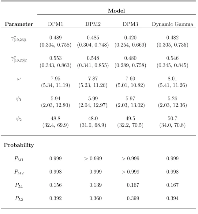
4.4 Chemoprevention Application . . . 47
4.4.1 Data Analysis . . . 47
4.5 Discussion . . . 56
5 NONPARAMETRIC BAYES TESTING OF CHANGES IN A RESPONSE DISTRIBUTION WITH AN ORDINAL PREDICTOR 58 5.1 Introduction . . . 58
5.2 Nonparametric Model and Prior Structure . . . 61
5.2.1 General Framework . . . 61
5.2.2 DMDP Model . . . 62
5.2.3 Model Space Prior . . . 64
5.2.4 Hyperpriors for DP Parameters . . . 66
5.3 Posterior Computation . . . 67
5.3.1 Full Conditional Posterior Distributions . . . 67
5.3.2 Hypothesis Testing . . . 69
5.3.3 Density Estimation . . . 70
5.4 Simulation Studies . . . 71
5.4.1 Description of Data . . . 71
5.4.2 Univariate Analyses . . . 72
5.4.3 Multivariate Analyses . . . 74
5.5 Genotoxicity Example . . . 74
5.5.1 Data and Methods . . . 74
5.5.2 Results . . . 77
5.6 Discussion . . . 78
6 CONCLUDING REMARKS 80 6.1 Overview . . . 80
6.2 Future Research . . . 81
A PROOF OF CONVERGENCE OF STAGE 1 CLUSTERING
ALGORITHM IN CHAPTER 3 83
B MCMC METHODOLOGY FOR CHAPTER 3 85
B.1 Methods for updating the random effects . . . 85 B.2 Methods for updating the hyperparameters . . . 86
C MCMC METHODOLOGY FOR CHAPTER 4 88
C.1 Full Conditional Posterior Distributions . . . 88 C.2 Updating Algorithm . . . 90
D MCMC METHODOLOGY FOR CHAPTER 5 92
LIST OF FIGURES
3.1 Plots used to elicit maximum radius, r, for CPP data. . . 23 3.2 Dirichlet process clustering of CPP data. . . 38 3.3 Mean smoking effects in the CPP data. . . 39 4.1 Posterior means and pointwise 95% credible intervals for hazard ratios
in chemoprevention study of canthaxanthin. . . 50 4.2 Posterior mean frailty trajectories for rats in the chemoprevention study. 52 4.3 Observed and predicted weekly tumor incidence prior to sacrifice for rats
in chemoprevention study. . . 53 4.4 Comparison of predictive frailty distributions obtained under different
priors. . . 55 5.1 Marginal density of y1 at each predictor level in simulation cases 2 and 3. 73
LIST OF TABLES
3.1 Means and 95% credible intervals for K and βb(∗) from simulation case 1. 30
3.2 Summary of Stage 2 clusters from simulation case 1. . . 31 3.3 Means and 95% credible intervals for K and βb(∗) from simulation cases
2 and 3. . . 32 3.4 Population effects of smoking in CPP analysis. . . 36 4.1 Sensitivity analysis of parameter estimates and posterior probabilities
CHAPTER 1
INTRODUCTION
In many analysis settings, the observed data do not possess the characteristics of a known distribution. For example, count data can often have a larger proportion of zeros than would be anticipated under the Poisson distribution (Carota and Parmigiani, 2002; Dunson, 2004). Time to event data can also have characteristics such as non-monotone hazards that contradict the behavior of parametric models such as the Weibull. When violations of assumptions are minor, fully parametric methods should be adequate, but in more extreme cases these methods can be overly restrictive making inferences questionable.
Such problems have motivated the vast literature on nonparametric statistical meth-ods. Robust frequentist methods exist for conducting two-sample tests (e.g., the Wilcoxon and Kolmogorov-Smirnov tests) and estimating distributions (e.g., the Ka-plan Meier and Nelson-Aelen estimates of the survival function and cumulative baseline hazard). Semiparametric regression models also exist which only require assumptions regarding the link function between covariates and the response. For example, Cox’s partial likelihood (1975) can be used to estimate regression coefficients in the propor-tional hazards model without assuming a specific distribution for the event times.
when appropriate and to move away from it when its fit is poor. Bayesian computation, often through the use of Markov chain Monte Carlo (MCMC) methods (Gelfand and Smith, 1990; Tierney, 1994), provides exact posterior estimates of the unknown dis-tribution as well as parameters and other functionals of interest. Frequentist methods typically rely on asymptotic evaluations which can be particularly troublesome in non-parametric settings where the number of unknown parameters increases with sample size.
Despite the promise of Bayesian nonparametric methods, computation can be diffi-cult. Advances in Gibbs sampling methodologies (e.g., MacEachern, 1994; West et al., 1994; MacEachern and M¨uller, 1998; Neal, 2000) have made Bayesian nonparametrics more feasible, but these approaches have some limitations. In particular, the commonly used P´olya urn sampler for Dirichlet process mixture models (MacEachern, 1994; West et al., 1994) is not computationally feasible for large data sets, such as those from multi-center longitudinal studies. Variational approaches (Blei and Jordan, 2006) are more efficient for large samples, but do not use true posterior distributions for inference. Another limitation of Bayesian nonparametrics is its lack of breadth. For instance, there are very few nonparametric or semiparametric Bayesian methods for multiple event time data. These data are common in biomedical studies in which the event of interest may be repeated infections, hospitializations, or recurrences of disease. Some examples include chemoprevention and cocarcinogenicity studies measuring the rate of appearance of palpable tumors of the skin and breast of animals exposed to a known carcinogen (Dunson, 2000; Gail et al., 1980; Forbes and Sambuco, 1998). Current meth-ods for analyzing these of data, such as the shared frailty model (Vaupel et al., 1979; Clayton and Cuzick, 1985), account for correlations between tumors from the same animal using random effects. However since animal-specific susceptibility may unex-pectedly change with age, generalizations of these models are needed to allow frailties to vary dynamically; ideally, such methods would be nonparametric and computationally efficient.
In this dissertation, we provide an introduction to Bayesian nonparametric inference and propose three semiparametric methods which address some of the computational, modelling, and testing issues mentioned above.
In Chapter 2, we provide a literature review of Bayesian nonparametric priors with particular attention given to the Dirichlet process and other priors used in hierarchical models and survival analysis.
In Chapter 3, we describe an empirical Bayes method which makes fitting semi-parametric random effects models feasible for large data sets. The method uses expert elicitation to construct a smaller set of pseudo-data which summarizes the scientifically important differences in the response and predictor values. We then fit a random effects model to the pseudo-data, assigning a nonparametric Dirichlet Process prior (DPP) to the random effects. This method was motivated by data from the Collaborative Peri-natal Project (CPP), which was a prospective epidemiology study consisting of over 30,000 children.
In Chapter 4, we propose a semiparametric dynamic frailty model for multiple event time data, which is motivated by data from studies of tumorigenesis. The model presents many interesting innovations over current methods including a computation-ally simple method of introducing correlation amongst time dependent frailties, piece-wise constant hazards, and dynamic regression coefficients. We also relax our assump-tions on the frailty using DPPs. To illustrate our method, we analyze data from a cancer chemoprevention study.
In Chapter 5, we discuss a Bayesian nonparametric method for testing for changes in a response distribution across an ordinal predictor, such as dose. Using a dynamic mixture of Dirichlet processes (DMDP; Dunson, 2006), we allow the response distribu-tion to change flexibly at each level of the predictor. In addidistribu-tion, we assign hierarchical priors to the mixture weights to obtain probabilities of no effect of the predictor and to identify thresholds in toxicology data, such as the lowest observed adverse effects level (LOAEL). The method also provides a natural framework for performing tests across multiple outcomes. We apply our method to simulated data and real data from a genotoxicity experiment.
CHAPTER 2
BAYESIAN NONPARAMETRIC
INFERENCE
Using the notation of Walker et al. (1999), letY1, . . . , YN iid
∼F be defined on some space Ω. In the Bayesian parametric framework, F would be a known distribution function, PΘ, and priors would be assumed for the unknown parameters Θ. Nonparametric
inference presents a different line of thinking in thatF is treated as an unknown function with prior PΩ.
2.1
The Dirichlet Process
2.1.1
General Framework
The Dirichlet process was originally introduced by Ferguson (1973, 1974) as a conve-nient method of eliciting a nonparametric prior forF using the Dirichlet distribution, which we now define. For a (k −1)-dimensional vector of positive random variables, (z1, . . . , zk−1), the (k−1)-variate Dirichlet distribution, Dirichlet(α1, . . . , αk) is defined
by the joint density
f(z1, . . . , zk−1) =
Γ(α)
Qk
j=1Γ(αj)
k−1 Y
j=1
zαj−1
j
1−
k−1
X
j=1
zj
αk−1
, (2.1)
wherePk−1
j=1zj ≤1,α =
Pk
j=1αj, and
E(Zj) =
αj
α Var(Zj) =
αj(α−αj)
α2(α+ 1) . (2.2)
Now consider the disjoint subsets of Ω, B1, . . . , Bk, where Ω =
Sk
j=1Bj. For an
axis of values, B1, . . . , Bk can be thought of as the set of non-overlapping intervals
which comprise the axis. The Dirichlet process prior (DPP), F ∼ DP(α0F0), assumes
that (F(B1), . . . , F(Bk)) has a Dirichlet distribution with parameters (α0F0(B1), . . . ,
α0F0(Bk)), where F0 is a known distribution, or base measure, and α0 is a precision
parameter which accounts for deviations from this parametric structure. As shown by Ferguson (1973), the posterior distribution of F is also a Dirichlet process with parameterα0F0+N·FN, whereFN is the empirical cdf. Thus, by choosing a smallα0,
representation of the DP where G∼DP(α0G0) implies that
G= ∞
X
i=1
wi(v)δθi
θi
iid
∼G0 and wi(v) = vi
Y
j<i
(1−vj) wherevj
iid
∼Beta(1, α0), (2.3)
δθi denotes a point mass at θi, and v ={v1, v2, . . .}. The mixing proportions wi(v) in
the above representation are generated by successively breaking a “stick” of unit length into an infinite number of pieces, and thus (2.3) is often referred to as thestick-breaking representation of the DP. This representation makes it clear thatGis discrete under a DPP, a result that was previously shown by Blackwell (1973).
2.1.2
Dirichlet Process Mixture (DPM)
The discrete nature of the DP is obviously problematic under a continuous Y. A simple solution to this problem is to use a Dirichlet process mixture or DPM (Antoniak, 1974). Consider a random vectoryi of lengthni whose distribution,F, is known and dependent
upon a set of latent variables φi. In a Dirichlet process mixture, the DPP is shifted
toφi to ensure that yi has a continuous distribution while still relaxing distributional
assumptions. Thus, the model has the following hierarchical structure:
yi|φi ∼ F(·;φi)
φi|G ∼ G (2.4)
G|α0,ψ0 ∼ DP
α0G0(·;ψ0)
,
where ψ0 are the parameters of the parametric base measure G0. Using the
stick-breaking representation of the DP, the DPM can also be described by the following process:
yi|zi ∼F(·;θzi) zi|v∼Multinomial(w(v)) i= 1, . . . , N
vj|α0 ∼Beta(1, α0) θj|ψ0 ∼G0(·;ψ0) j = 1,2, . . . , (2.5)
where zi indicates the mixture component with which yi is associated and w(v) =
{w1(v), w2(v), . . .}.
was to provide nonparametric estimates of normal means. The hierarchical structure of this model is simply Yi ∼ N(µi, σ2), µi ∼G, and G∼DP(α0G0). Other authors have
used the DPM for density estimation (e.g., West et al., 1994; Escobar and West, 1995) and to construct semiparametric hierarchical models, as discussed in Section 2.1.4.
As noted by Neal (2000), sometimes a Dirichlet process mixture is referred to as a Mixture of Dirichlet processes (MDP) in the literature because the full conditional posterior of G is an MDP (Antoniak, 1974). However, this characterization will be avoided since models are usually characterized by their prior distributions and not their posteriors (Neal, 2000).
2.1.3
Computation under the DPM
P´olya Urn Gibbs Sampling
As mentioned earlier, the P´olya urn representation of the DP (Blackwell and MacQueen, 1973) has motivated Gibbs sampling methods for the DPM. Given Φ={φ1, . . . ,φN}
constitute a set of exchangeable random variables, when G is integrated over its DPP it can be shown that Φmay be generated according to the sequence (Escobar, 1994):
φ1 ∼ G0
φ2|φ1 ∼
αG0 +δφ1
α0+ 1
.. .
φN|φ1, . . . ,φN−1 ∼
αG0 +PN
−1
j=1 δφj
α0+N −1
, (2.6)
As noted by West et al. (1994), any realization of φ1, . . . ,φN lies in a set of K ≤ N
distinct values or clusters, with common valuesθ={θ1, . . . ,θK}. Thus, the conditional
prior of φi given φ
(i)
i ={φj :j 6=i}is:
α0
α0+N −1
G0+
1 α0+N −1
K(i) X
j=1
n(ji)δθ(i) j
, (2.7)
From (2.7), the full conditional posterior of φi follows immediately
π(φi|Y,φ
(i)
i ) =qi0Gi0+
K(i)
X
j=1
qijδθ(i) j
, (2.8)
whereY denotes the total data and each qij is a multinomial probability given by
qij =
(
c·α0hi(yi) j = 0
c·n(ji)fj(yi|θj) j >0,
where
• Gi0is the posterior obtained by updating the base measureG0with the likelihood,
or equivalently
dGi0(φi)∝fi(yi|φi)dG0(φi),
• hi(yi) is the observed value of the marginal density ofyi under the base measure,
hi(yi) =
Z
fi(yi|φi)dG0(φi)
• c is a normalization constant
The predictive distribution of a futureφi,φN+1 is also easily obtained under the P´olya
urn representation of the DP,
π(φN+1|φ) =
α0
α0+N
G0+
1 α0+N
K X
j=1
njδθj. (2.9)
For more details on these prior, posterior, and predictive distributions, please see MacEachern (1994) and West et al. (1994).
As demonstrated by Escobar (1994) and Escobar and West (1995), posterior com-putation may proceed using a Gibbs sampling algorithm which updates Φ from (2.8). However, this approach is subject to slow mixing sinceθis rarely updated. Thus, based on the initial ideas of MacEachern (1994), West et al. (1994), propose a more efficient algorithm which updates the number of clusters (K), the configuration of subjects, and the unique values at each iteration of the MCMC. LetS={S1, . . . , SN} define a set of
follows from (2.8),
P(Si =j|Y,θ(i)) =qij. (2.10)
Thus, the sampling algorithm proceeds as follows:
1. Given the values of θ and S obtained from the previous iteration of a Gibbs sampler, sample S1, . . . , SN from (2.10) with a new φi drawn from Gi0 when
Si = 0.
2. Given the updated values of K and S, update θ using the posteriors, π(θj|Y,S)∝
Y
i:Si=j
fi(yi|θj)
dG0(θj), (2.11)
forj = 1, . . . , K.
The computational ease of DPMs depends upon whether or not the base measure is conjugate; i.e., doesG0 result inGi0 from the same family of distributions. WhenG0 is
conjugate,hi(yi) has a closed form and posterior computation is simple using the above
sampling algorithm. However, when conjugacy does not hold, more complex sampling algorithms must be used. West et al. (1994) proposed estimatinghi(yi) using either
nu-merical quadrature or a Monte Carlo simulation which uses the average value off(yi|φi)
over several values of φi sampled from G0. An alternative method was proposed by
MacEachern and M¨uller (1998) which avoids numerical integration. Under their ap-proach, N candidate atoms are sampled from G0 at each iteration: θK+1, . . . ,θK+N.
If n(li) > 0 for subject i currently in cluster l, then φi is sampled according to the
probability function,
π(φi|θ(i),Y)∝
α0
K+ 1
f(yi|θK+i)δθK+i +
K
X
j=1
qijδθj, (2.12)
else if n(li) = 0, φi is unchanged with probability (K −1)/K and with probability
Other Methods
Although P´olya urn sampling methods are easy to implement, in some situations they can be slow to converge and mix poorly, even when MacEachern’s (1994) and West et al.’s (1994) algorithms are used. For instance, Jain and Neal (2004) note that when two or more mixture components have similar parameter values, the Gibbs sampler can become trapped in a local mode that corresponds to an incorrect clustering of data points. To address this issue, Jain and Neal proposed a Metropolis-Hastings procedure which increases the efficiency of cluster assignment by splitting and merging entire clusters at each step of the MCMC.
Another limitation of the P´olya urn sampling methods is that they do not provide direct samples from the DP. As a result, one cannot estimate credible intervals for the functional assigned the DPP. To address this issue, several authors have proposed com-putational algorithms which sample from a truncated version of Sethuramans’ (1994) stick-breaking representation. For instance, Ishwaran and James (2001) proposed a blocked Gibbs sampler which updates the atoms, weights, and remaining hyperparam-eters from their joint distributions. For related approaches see Muliere and Tardella (1998), Ishwaran and James (2002), and Gelfand and Kottas (2002).
Some other computational methods for DPMs include alternatives to MCMC sim-ulation. For example, importance sampling-type methods have been proposed by Liu (1996) and MacEachern et al. (1999). Newton and Zhang (1999) also proposed a predictive recursion method for estimating predictive distributions. Although these approaches are faster than Gibbs sampling, the importance sampling methods can pro-duce large Monte Carlo error and predictive recursion tends to over-smooth (see, e.g., Quintana and Newton, 2000).
Recently, Blei and Jordan (2006) proposed a Variational Bayes (VB) approach to in-ference for the DPM. Under the stick-breaking representation (2.5), letz= (z1, . . . , zN)0
denote the mixture indicators forN subjects. The VB approach replaces the joint pos-terior of the stick-breaking parameters,π(v,θ,z|Data), with a variational distribution which truncates the stick-breaking process at M atoms:
q(v,θ,z) =
M−1
Y
m=1
Beta(vm;am, bm) M
Y
m=1
q∗(θm;ηm) N
Y
i=1
Multinomial(zi;πm), (2.13)
where q∗() denotes a distribution in the exponential family and am, bm,ηm,πm m =
lower bound on the log-marginal likelihood. As opposed to MCMC, VB has a single optimization criterion that can be used to assess convergence. In addition, Blei and Jordan have provided empirical evidence that VB is much faster than MacEachern’s (1994) Gibbs sampler and Ishwaran and James’ (2001) blocked Gibbs approach. How-ever, a major disadvantage of this method relative to the MCMC approaches is that the estimates from VB are based on an approximation instead of the true posterior.
Hyperparameter estimation
As mentioned above, the base measure in the DPM, G0, is usually fixed or assumed to
come from a parametric family of distributions with a fixed hyperprior placed on its parameters,Ψ0 (see, e.g., West et al., 1994; Escobar and West, 1995; MacEachern and
M¨uller, 1998). However, some authors have considered nonparametric estimation ofG0.
For instance, some have assigned DPPs (e.g., Teh et al., 2006) or DPMs (e.g., Tomlinson and Escobar, 1999) to G0. MacAuliffe et al. (2006) describe another approach in
whichG0 is estimated everyT∗ iterations of the MCMC using kernel density estimates
constructed from θ.
A few authors have also proposed methods for estimating α0 from the data. For
example, West (1992) assigned a gamma prior to α0, while Carota and Parmigiani
(2002) proposed a regression model. Liu (1996) developed sequential imputation and Gibbs sampling methods for approximating the MLE of α0 (see also MacAuliffe et al.,
2006).
2.1.4
Random Effects Modelling
The computational methods developed for DPMs have made nonparametric modelling of random effects feasible. For instance, when a DPP with a normal base measure is assigned to the unknown distribution of a random block effect (e.g., Bush and MacEach-ern, 1996) or a random coefficient (e.g., Kleinman and Ibrahim, 1998) in a linear model, conjugacy is achieved and computation may proceed using West et al.’s (1994) method. Hierarchical count data can also be modelled by a conjugate DPM by specifying a gamma base measure in the DPP for the random effect distribution (see, e.g., Dunson, 2004). However, as discussed in Mukhopadhyay and Gelfand (1997), a conjugate G0
Although DPMs improve the flexibility of random effects models, smoothness of the random effect distribution is compromised due to the almost surely discrete restriction of the DPP. However, this problem can be fixed by adding another level of hierarchy to the model; i.e. one may assume thatGis fixed given the latent variables νi and assign
a DPP to the unknown distribution of νi. For example, M¨uller and Rosner (1997) use
a DPM to model subject-specific coefficients within a nonlinear model for blood count data.
Some authors have developed generalizations of the DP to allow the distributions of random effects or other latent variables to depend on covariate values. For exam-ple, dependent nonparametric processes have been proposed by Cifarelli and Regazzini (1978), MacEachern (1999, 2000), M¨uller et al. (2004), Dunson (2006), and Dunson and Pillai (2004). In Chapter 5, we will discuss these methods in more detail and propose a generalization of the Dunson (2006) approach.
2.2
The P´
olya Tree
2.2.1
General Framework
Another common nonparametric prior is a generalization of the Dirichlet process known as the P´olya tree or PT for short(Ferguson, 1974; Lavine, 1992, 1994). The P´olya tree is defined by an infinite set of binary partitions of the space Ω. LetB0andB1be obtained
by splitting Ω into two pieces. B0 and B1 are split into (B00, B01) and (B10, B11),
respectively, and this process is repeated ad infinitum. For some m, let = 1· · ·m
with k ∈ {0,1} for k = 1, . . . , m so that defines a unique set of partitions, B. A
random probability measure F on Ω is said to have a P´olya tree prior if there exists nonnegative numbersA= (α0, α1, α00, . . .) and random variablesC = (C0, C00, C10, . . .)
such that
1. All random variables in C are independent
2. For every ,C0 ∼Beta(α0, α1)
3. For every m = 1,2, . . . and every =1 · · ·m,
F(B1...m) =
m Y
j=1;j=0
C1···j−10
m
Y
j=1;j=1
(1−C1···j−10)
where the first terms (for j = 1) are interpreted as C0 and 1 −C0 (Lavine, 1992).
The formal shorthand notation is F ∼ PT(Π,A), where Π is the set of partition probabilities.
An attractive feature of the P´olya tree prior is that it is conjugate, i.e. F|Y ∼ PT(Π,A|Y), where A|Y=α+n and n is the number of observations from Y inB
(Ferguson, 1974; Lavine, 1994). Thus, wheny1, . . . , yN are all uncensored, the posterior
predictive distribution of a future observation,YN+1, follows immediately
P(YN+1 ∈B) = m
Y
k=1
α1···k +n1···k
α1···k−10+α1···k−11+n1···k−1
. (2.15)
2.2.2
Applications
A P´olya tree priors can be centered on a probability distribution, F0, by taking the
partitions to coincide with percentiles ofF0 and assuming that α0 =α1 =α for each
(Lavine, 1992). At levelm, this would correspond to the partitions Bj ={(F0−1 (j−1)/2m
, F0−1 j/2m} for j = 1, . . . ,2m, where F0−1(0) = −∞ and F0−1(1) = ∞. To facilitate computation, C is terminated at some finite level M and attention is restricted to the r = 2M partitions given by π
M = (B1, . . . , BM) (Lavine,
1992).
Some additional attention must be given to the choice of α. As seen in (2.15), as
α decreases for each m, the posterior predictive distribution of YN+1 approaches the
empirical cdf. Thus, in this sense, α is similar to the parameter α0 in the DP in that
it quantifies the prior confidence in the base distribution. However, interpreting α as
a precision parameter is limiting since it also determines the smoothness ofF (Lavine, 1992). To see this trait, consider the probability of twoYi’s taking on the same value,
P(Yi =y|Yj =y) =
∞
Y
k=1
α1···k + 1
α1···k−10+α1···k−11+ 1
. (2.16)
According, to Mauldin et al. (1992), (2.16) equals 0 is a sufficient condition for a continuous F, which can be approached by allowing α to increase with m. Ferguson
(1974) claims that α = m2 implies that F is continuous with probability one, which
Lavine (1992) calls a “sensible canonical choice” for α. Alternatively, the P´olya tree
may be specialized to the Dirichlet process by choosingα =α/(2m), but as mentioned
previously, this ensures that F is discrete (Blackwell, 1973; Ferguson, 1973).
censoring times to maintain conjugacy (Muliere and Walker, 1997). Thus in order to center the tree on a given distribution, Muliere and Walker (1997) propose setting each α = γmF0(B), where γm is a constant. This method not only ensures that
E(F(B)) =F0(B), but it also allows one to specify γm such that the continuity ofF
is ensured. In addition, the predictive probabilities retain a simple form,
P(YN+1 ∈B) = m
Y
k=1
α1···k +n1···k
α1···k−10+α1···k−11+n1···k−1 −s1···k−1
, (2.17)
wheres1···k−1 is the number of observations censored in B.
In some recent applications, P´olya tree priors have been used to model random error or subject-specific random effects in semiparametric regression models. For example, Walker and Mallick (1997) assigned P´olya tree priors to random effects in hierarchical generalized linear models and frailty models. Although the full conditional posterior of F is tractable, the conditional posteriors of the random effects are not. Thus, computa-tion requires either an indirect sampling method to obtain values of the random effects (e.g., Metropolis sampling) or constructing additional latent variables to achieve conju-gacy. These methods are more computationally intensive than the P´olya urn sampling methods for the DPM.
Another disadvantage of the P´olya tree is its sensitivity to the choice of partitions. This latter problem may be alleviated by using a mixture of P´olya trees in which the parameters of the centering distribution,F0, and/orA are random. This approach also
improves computational efficiency since it does not require one to choose F0 with a
large enough variance to cover the support of F. Hanson and Johnson (2002) used a mixture of P´olya trees in an accelerated failure time model.
2.3
Independent and Dependent Increments Models
2.3.1
Neutral to the Right Processes
The Dirichlet process is also a special case of a general set of nonparametric priors known as neutral to the right (NTTR) processes. As defined by Doksum (1974), a distribution function, F(t), is NTTR if it can written in the form F(t) = 1−e−Y(t)
whereY(t) is a process with independent increments and
2. Y(t) is right continuous a.s. 3. limt→−∞Y(t) = 0 a.s. 4. limt→∞Y(t) =∞ a.s.
Y(t) has at most a countably finite number of discontinuity points t1, t2, . . . with
independent jumps W1, W2, . . . NTTR priors are generally specified in terms of the
differences
Z(t) = Y(t)−X
j
Wj1(tj ≤t <∞),
which do not have any points of discontinuity. As is the case with PT priors, NTTR priors are always conjugate (Doksum, 1974).
Some special cases of NTTR processes have proven to be useful in Bayesian sur-vival analysis. For example, Kalbfleisch (1978) used a special NTTR process known as the gamma process to develop a semiparametric proportional hazards model. In Kalbfleisch’s model, Y(t) = Λ0(t), the cumulative baseline hazard function, and Z(t)
is the increment in Λ0(t) at time t. Using a finite set of partitions of the time axis,
0 < τ1 < · · · < τM < ∞, Z(τj) iid
∼ Ga(c0z0(τj), c0) where z0(τj) is an initial guess at
the true value of the increment andc0 is a precision parameter forj = 1, . . . , M. Hjort
(1990) also developed discrete time and continuous time beta process priors for the increments in the cumulative baseline hazard. The gamma and beta processes are easy to implement (due to conjugacy) and provide a simple structure for incorporating a priori knowledge about the hazard function into analyses.
2.3.2
Dependent Increments Models
Although NTTR priors have some nice properties, the independent increments assump-tion may not be reasonable in some settings. In particular, one would typically expect the hazards from adjacent time intervals to be correlated a priori. To address this issue, some authors have proposed generalizations. Letλ0j denote the baseline hazard
over the jth partition of the time axis. To induce correlation, Aslanidou et al. (1998) modelled the baseline hazard using the discrete time martingale process of Arjas and Gasbarra (1994):
λ0j|λ01, . . . , λ0(j−1) ∼Ga
ν, ν λ0(j−1)
In (2.18), the smoothness of the baseline hazard is controlled by the value of ν. Sinha (1998) proposed an alternate model for the baseline hazard which uses a correlated process described by Gamerman (1991):
log(λ0(j+1)) = log(λ0j) +ej+1 ej+1 ∼N(0, σ2). (2.19)
CHAPTER 3
EMPIRICAL BAYES FITTING
OF SEMIPARAMETRIC
RANDOM EFFECTS MODELS
TO LARGE DATA SETS
3.1
Introduction
MIXED failed to converge.
When a data set is large, as in the CPP, it would also be advantageous to use the abundant information to relax assumptions of models, such as normality of random effects. Bayesian nonparametric or semiparametric methods are attractive in these settings since the random effect distribution can be assigned a prior which reflects a priori knowledge about the shape or location. For instance, a Dirichlet process prior (DPP) may be assigned to the random effect distribution (see, for example, West et al., 1994, Bush and MacEachern, 1996, Mukhopadhyay and Gelfand, 1997, and Kleinman and Ibrahim, 1998), which reduces the number of random effects to a set of K ≤ N unique values. Each of these K clusters represent subjects with common latent traits which may include interesting genetic or environmental factors worthy of future study. Despite the promise of the DPP, K increases rapidly with N which can lead to a scientifically implausible and computationally impractical number of clusters when N is very large.
Unfortunately, few authors have considered adapting the computational methods for the DPP to handle large data sets. Although Blei and Jordan’s (2006) variational inference method can substantially reduce computation time, especially for large N, the approach relies on replacing the true posterior density with a lower bound having unknown accuracy. Potentially, the particle filtering methods described by Chopin (2002), Ridgeway and Madigan (2003), and Balakrishnan and Madigan (2006) could be generalized to make Bayesian nonparametric inference feasible for large data sets. In this paper, we consider an alternate approach which involves scaling-down the size of the data prior to performing MCMC. Existing methods fordata squashing include methods which fit models to both real and generated data, also known as pseudo-data, which are representative of the complete data. For example, DuMouchel et al. (1999) and Madigan et al. (2002) construct pseudo-data using a moment matching and likelihood-based approach, respectively, while Owen (2003) uses a random sample of the complete data. Huang et al. (2005) proposed a related Bayesian method for fitting hierarchical models, though their approach is parametric and involves combining posteriors from several sub-samples of the data.
signifi-cant by an expert of the subject matter. In the second stage, we use a DPP to model the G cluster means, further clustering the groups from the first stage. By applying the DPP to the cluster means instead of the complete data, we reduce both the com-putation time and the number of latent classes. In addition, our use of expert opinion improves the scientific justification of clustering. For discussion of the importance of expert elicitation, refer to Kadane and Wolfson (1998), Meyer and Booker (2001), and Garthwaite et al. (2005).
In Section 3.2, we discuss the CPP data and previous results. In Section 3.3, we propose the method. Section 3.4 contains a series of simulation examples, Section 3.5 applies the approach to the CPP data, and Section 3.6 discusses the results.
3.2
Maternal Smoking and Childhood Growth Data
As described by Broman (1984), the Collaborative Perinatal Project (CPP) was a large prospective study of pregnancy and childhood development. The study consisted of 55,043 pregnancies enrolled at 12 study centers in the U.S. between 1959 to 1965 and included measurements obtained from children starting at birth and concluding at age 8. The investigators targeted 20 different outcomes in the study including the presence of mental and communicative disorders in the children and physical growth.
The CPP measured smoking during pregnancy and child height and weight at fol-lowup visits. Chen et al. (2006) used the measurements at birth and at years 1, 3, 4, 7, and 8 to determine the effects of maternal smoking on childhood growth amongst 34,866 children (17,348 boys and 17,518 girls). Categories of smoking exposure included (1) never smoked, (2) ex-smokers, and (3) currently smoking based on questionnaire data at registration or subsequent prenatal visits. Being unable to implement random effects models due to the large sample size, the authors used GEE to demonstrate that mothers who smoked during pregnancy had infants with lower birth weight, but by age 8, these children had a greater risk of being overweight.
3.3
Methods
3.3.1
General Motivation
Fori = 1, . . . , N, let yi = (yi1, . . . ,yin
i)
0 denote a set of n
i longitudinal measurements
on subject i. Letting Xi = (xi1, . . . ,xip) denote a set of predictors, we focus on the
linear random effects model
yi|bi,Xi
∼N Xibi, τ−1Ini
, (3.1)
where Ini is an ni × ni identify matrix and bi = (bi1, . . . , bip)
0 ∼ H, an unknown distribution with meanβ and covariance V.
As N becomes very large and both ni and p remain modest, many subjects have
essentially identical values withyi ≈yj andXi ≈Xj for many different pairsi, j.
Out-comes, such as weight, that are treated as continuous are often truncated or rounded when recorded, limiting the number of unique values in the data. In addition, val-ues which are so close that a subject matter expert would consider them scientifically indistinguishable can be grouped together without loss of important information. Un-der these circumstances, the data are adequately summarized by values for G << N clusters. For an observationi in cluster g let
ygi =yg+gi
Xgi=Xg+∆gi bgi =bg +φgi (3.2)
whereyg,Xg, andbg are the cluster-specific means of the response, predictors, and
ran-dom effects,gi and φgi are random variables, and∆gi is a matrix of constants. When
the G clusters adequately represent the heterogeneity in the data, the observed values of gi, φgi, and ∆gi are all approximately zero. Thus, β = E(bi) can be reasonably
estimated by
b
β= 1 N
N
X
i=1
bi =
1 N G X g=1 X
i∈g
(bg+φgi)≈
1 N
G
X
g=1
mgbg =βe, (3.3)
wheremg is the number of subjects in cluster g.
3.2, we recommend a strategy for initial clustering of the N subjects in G groups. In Section 3.3, we propose a flexible Stage 2 clustering procedure which uses a DPP to avoid restrictions onH. Section 3.4 describes the MCMC algorithm and in Section 3.5 we discuss our approach to inference.
3.3.2
Stage 1 Clustering
We propose a stratified methodology to generate the first stage clusters. Although related to the data-sphere method used by DuMouchel et al. (1999), our procedure is geared to the random effects problem and incorporates knowledge of subject matter experts. Subject-specific data are first divided into q strata based on categorical pre-dictors. For example, if there are two categorical predictors, one dichotomous and one with three levels,qshould equal 6. Within each stratum, we wish to develop clusters of scientifically indistinguishable subjects based on the values of the continuous variables, i.e., the longitudinal responses and continuous predictors. For subject i in stratum j, we denote the values of these variables as wji = (wji1, . . . ,wjipji)
0. For ease in exposi-tion, we will temporarily assume thatpji =pj fori= 1, . . . , Mj, wherepj is the number
of continuous variables for each subject in stratumj and Mj is the stratum frequency.
Prior to clustering, we transform wji tozji = (zji1, . . . ,zjipj)
0, where
zjik =
(wjik−wjk)
swjk
,
and wjk and swjk denote the mean and standard deviation, respectively, of the kth
continuous variable in stratumj.
Let the z-scores in stratum j be divided into Gj clusters whose location inpj-space
are represented by a set of data points orseeds,cj1, . . . ,cjGj, wherecjl= (cjl1, . . . ,cjlpj)
0
and cjlk is the average value of the kth standardized variable in cluster l. We assume
that both the number of clusters and locations are unknown a priori, but through expert elicitation, we define a threshold r such that
d(zji,cjl) =
v u u t
pj
X
k=1
(zjik−cjlk)2 ≤r (3.4)
cluster seed, or the maximum radius of a cluster.
To elicit r, we recommend performing a set of exploratory cluster analyses and presenting the results to one or more subject matter experts. These analyses may be performed using a set of historical data, or alternatively, one stratum of the current data. In the latter method, the data used to elicit r will also be used in the second stage of the analysis, thus creating a sort of an empirical Bayes approach. In our analysis of the CPP data, we treated the data on male children of never smokers as our historical data, and we used it to choose an appropriater for the female subjects. In our exploratory analyses, we used a range of r values to cluster the longitudinal weight of males with complete data (i.e., with followups at ages 0, 1, 3, 4, 7, and 8). Following each analysis, we plotted the growth curves from subjects in the cluster with largest radius (see Figure 3.1). Using these plots, we asked a panel of experts on body weight research (2 MD’s, a PhD in Nursing, and an Exercise Physiologist) to tell us which clusters (each indexed by a radius, r) contain curves with potentially significant differences. In our example, 3 out of 4 panel members agreed that when r ≤ 2.14, the growth curves in each cluster were not significantly different. Thus, r = 2.14 was the obvious choice for the CPP. In other applications where there is substantial disagreement across the experts, the average elicited value could be used instead. Our method for choosing r is similar to the use of opinion pools to combine probability distributions elicited by several experts; for an example see Cooke and Goossens (2000).
Once we have specified r, we apply the following three-step methodology to cluster the continuous data in stratum j:
Step 1. Initialize cluster seeds. InitializeGjat 1 and letc
(0)
j1 =zj1. Fori= 2, . . . , Mj, ifd∗ji = minld(zji,c
(0)
jl )> r,
then incrementGj by 1 and define a new seed, c
(0)
jGj =zji.
Step 2. Iteratively update the seeds. Initialize an index variable, t, at 1 and perform the following steps:
2.1 For i= 1, . . . , Mj, if d∗ji ≤r assign zji to the cluster with the closest seed.
2.2 For l= 1. . . , Gj compute
c(jlt) = 1 mjl
X
i∈j,l
where mjl is the number of subjects currently in cluster j, l. Let 0≤ν <1
denote a pre-specified convergence criterion such that changes in the cluster seeds less than or equal to ν ·d∗j0 are permissible, where d∗j0 denotes the minimum distance between the initial seeds. If maxld(c(jlt),c(t
−1)
jl ) > ν·d
∗
j0,
then increment t by 1 and repeat Steps 2.1 and 2.2, otherwise proceed to Step 3.
Step 3. Construct final clusters.
3.1 Repeat Step 2.1 using c(jt1), . . . ,c(jGt)
j.
3.2 For all i : d∗ji > r, assign zji to its own cluster and update the value of Gj
accordingly.
Step 1 of our method is related to the leader algorithm (Hartigan, 1975), while Step 2 can be thought of as a form of k-means clustering (MacQueen, 1967) since the cluster seeds are the means of the observations assigned to each cluster when the algorithm is iterated until complete convergence (i.e., ν = 0). A proof of convergence of our algorithm is provided in Appendix A. After completing Steps 1-3 for j = 1, . . . , q, we compute the means of the untransformed variables in each cluster, wjl =
P
i∈(j,l)wji.
As mentioned in Section 3.1, these data (plus the values of any categorical predictors) will constitute ourG=Pq
j=1Gj pseudo-subjects.
The above method is attractive for many large data sets since it leads to the quick formulation of first stage clusters chosen to have minimal scientifically-important dis-tances between them. By choosing r based on expert elicitation, we induce a prior on the clustering process. Our initialization method then uses this prior to identify the most important separations in the data. Another attractive feature of our method is that all three steps may be implemented using PROC FASTCLUS (SAS, version 9) and sample code is available upon request from the authors.
In many longitudinal studies, including the CPP,pji 6=pji0 for several pairs (j, i),(j, i0)
based on adjusted distances,
dadj(zji,cjl) =
rp
j
pji
X
(zjik−cjlk)2, (3.5)
where the sum is taken over thepji nonmissing variables for subject i in cluster j. As
before, these subjects may still be assigned to their own cluster if d∗ji > r in Step 3, and thus, we do not ignore any important outliers.
3.3.3
Dirichlet process clustering
In the remaining sections of this chapter, we will drop the stratum index from the Stage 1 clusters and refer to the pseudo-data as (y∗1,X∗1), . . . ,(y∗G,X∗G). For pseudo-subject g = 1, . . . , G, we assume
[yg∗|X∗g,b∗g, τ]∼N(X∗gb∗g, τ−1In∗
g)
b∗g ∼H H ∼DP(αH0), (3.6)
wheren∗g is the number of measurements on pseudo-subjectg,H0 is a known
distribu-tion, andα is a precision parameter. In all the examples we will consider, H0 = N(µ,
D).
As discussed in Section 2.1.3, if we marginalize over the DPP for H, the sequence of random effects, b∗1, . . . ,b∗G, follows a Polya urn scheme (Blackwell and MacQueen, 1973), i.e.,
b∗k|b∗1, . . . ,b∗k−1
(
=b∗j with probability 1
α+k−1
∼H0 with probability α+αk−1,
(3.7)
for j < k and k = 2, . . . , G. Thus, under the DPP, the random effects are clustered into K ≤ G different groups whose random effects are θ1, . . . ,θK, where θl ∼ H0 for
l= 1, . . . , K (MacEachern, 1994).
Let S1,i ∈ {1, . . . , G} and S2,i ∈ {1, . . . , K} index the stage 1 and 2 clusters of
subject i, respectively. Given the frequencies of our Stage 1 clusters, m1, . . . , mG, the
probability that two, randomly selected subjects are in the same Stage 1 cluster is
Pi,i0 = Pr(S1,i=S1,i0) = G
X
g=1
mg
2
N
2
which follows from the multivariate hypergeometric distribution. Also, under the DPP, the probability that two pseudo-subjects are grouped together is 1/(α+ 1) (Antoniak, 1974). Therefore, a priori,
Pr(S2,i =S2,i0) = Pi,i0 +
1−Pi,i0
α+ 1 ≥ 1
α+ 1. (3.9)
Thus, our method increases the prior probability that two subjects are clustered to-gether, relative to a DPP applied toN subjects. As a result, our prior favors a smaller, but more scientifically justified, number of clusters.
3.3.4
Posterior Computation
Computation under the DPP proceeds using the West et al. (1994) P´olya urn sampler described in Section 2.1.3 and the details regarding both the full conditional posterior distributions of b∗1, . . . ,b∗G and the sampling algorithm are provided in Appendix B. The major difference between our implementation and the standard use of the sampler is that our conditional posteriors in terms ofG pseudo-subjects instead of N subjects. It is important to note that if we were to apply the DPP to N random effects, instead of G, the MCMC would iterate very slowly for large samples and computation may be infeasible. In addition, the large matrices needed to update values for N subjects can cause memory problems in certain software, such as Matlab. This latter difficulty prevented us from applying the DPP to each subject in the CPP data.
To reduce the sensitivity of the Stage 2 clustering to subjectively chosen hyperpa-rameters, we recommend placing hyperpriors on µ, D, τ, and α. For our models, we use the priors
π(µ) = N(µ0,Σ0) π(D−1) = W(d0,D0)
π(τ) = Ga(ψτ0, ψ) π(α) = Ga(a, b),
where W(·, d0,D0) is the Wishart density with degrees of freedom d0 and mean D0.
3.3.5
Methods for Inference
In Section 3.3.1 , we demonstrated that population-average effects,β, can be estimated by a weighed mean of b1, . . . ,bG. Although the DPP is applied to cluster means,
b∗1, . . . ,b∗G are computed based on one pseudo-subject and, as a result,
Cov 1 N X g=1
mgb∗g
>Cov(βe) =
1 NV.
However, givenβ, a transformation can be made, ˙
bg =m−g1/2b
∗
g+ (1−m
−1/2
g )β,
which preserves the mean forb∗g, but changes the covariance toV/mg so that
Cov 1 N G X g=1
mgb˙g
= 1 NV.
Based on the above results, we make a similar, posterior transformation ofb∗1, . . . ,b∗G, which ensures that the variance of the population effects is reflective of the cluster size. Following convergence, let b∗g(t) denote the value of b∗g observed at iteration t, t= 1, . . . , T. Prior to calculating the population mean, we replaceb∗g(t) with
e
bg(t) =m−g1/2bg∗(t)+ (1−m−g1/2)b∗g, (3.10)
whereb∗g =PT t=1b
∗(t)
g /T. Note that for largeT, Cov(b
∗
g) approaches0and, thus, we do
not (significantly) inflate the variances ofbeg by estimating the posterior mean. In the
special case wheremg=1, we simply havebe
(t)
g =b
∗(t)
g , and as the first stage cluster sizes
grow, we shrink back towards the mean of the samples. By doing shrinkage within the first stage clusters instead of across the clusters, we do not obscure or mask non-normal features in the random effect distribution.
Now that we have corrected our estimates of the cluster-specific means, population effects can be estimated at each iteration of the MCMC as
b
β((∗t))= 1 N
G
X
g=1
mgbe
(t)
g . (3.11)
effects of the predictors, similar to what is done with fixed effects in mixed models. Inferences about heterogeneity can be based on the posterior clustering of the ran-dom effects. As in Bigelow and Dunson (2005), the Dirichlet process clustering can be summarized by post-processing the results from the MCMC using a hierarchical cluster-ing procedure such as scluster-ingle linkage, which is also known as nearest-neighbors (Sneath, 1957). In this paper, we define a new set of Stage 2 clusters k = 1, . . . , K∗ where for each pseudo-subjectg in clusterk, there exists some other pseudo-subject g∗ such that Pr(Sg = Sg∗) ≥ p∗, where, under the West et. al (1994) sampling algorithm for the
DPM, Sg indicates the cluster membership of pseudo-subject g. To ensure adequate
separation between our clusters, we choose p∗ = 0.5 in our analyses. This clustering procedure can be implemented using the linkage and cluster functions in MATLAB (version 6). As seen in our analysis of the CPP data, the cluster-specific longitudinal trajectories and the proportion of subjects per cluster are useful in identifying outliers in the data.
3.4
Simulation Studies
We applied the approach to three simulated data examples. In each case, the true model for yi given bi was yi ∼ N(Xibi,I6) where Xi = (xi0,xi1,xi2) with xi0 = 16,
xi1 = ui·16, ui ∈ {0,1}, andxi2 = (0,1,3,4,7,8)0/8 fori= 1, . . . , N. The predictorxi2
can be thought of as the age at followup for subject i and ui as an exposure indicator,
wherePN
i=1ui =N/2 in cases 1-3.
3.4.1
Case 1: Latent Class Data
In the first case, we simulated a single data set of size N = 2000 using the discrete distribution
bi =
θ1 = (2.26,0.46,20.35)0 with probability 0.0792
θ2 = (3.14,1.34,22.76)0 0.2969
θ3 = (3.30,1.50,23.20)0 0.3065
θ4 = (3.46,1.66,23.64)0 0.2969
θ5 = (4.77,2.97,27.23)0 0.0205,
which has meanβ = (3.25,1.45,23.06)0. We will refer to all i:bi =θj as Classj.
data). Diffuse priors were chosen forµandτ withµ0 = (15,0,0)0,Σ0 = 100·I3,τ0 = 1,
and ψ = 0.1. The prior for D was centered on the identity matrix, with d0 = 3. We
also letα ∼Ga(a,1) where we leta= 0.25 for r= 2.14 andr= 1.66, but chosea= 0.1 for the complete data to induce a similar prior forK acrossG. The MCMC was run for 25,000 iterations in each analysis with the first 5,000 iterations discarded as a burn-in and with every 10th sample collected to thin the chain. To speed up computation, we sampled each Sg conditional on the random effect values at the previous iteration.
Table 3.1 provides estimates ofK and the population effects from our MCMC. Both the number of clusters and the values of the regression parameters are similar across r. In addition, the elicited r reduced computation time by approximately 19 hours, relative to complete data, which demonstrates the efficiency of our method.
After post-processing the results of our MCMC using nearest neighbor clustering, we obtained 4 Stage 2 clusters. One cluster consisted of an outlier from Class 2 but, as seen in Table 3.2, the remaining clusters demonstrate good agreement with the subjects’ true clusters: one cluster consists of mostly Class 1 subjects, another is primarily comprised of subjects from Classes 2-4, while the third only contains subjects from Class 3. Thus, under the elicited r, our method effectively separated the extreme outliers (Class 5) from the rest of the data and, although less successful, was able to isolate most of the moderate outliers (Class 1). In addition, the parameter estimates within each cluster, βb(∗1),βb(∗2), and βb(∗3), are comparable to the true values within Classes 1,
2-4, and 5, respectively. Under r = 1.66 and r = 0, the parameter estimates of the three largest clusters were similar to those listed in Table 3.2. However, the number of singleton clusters increased as r decreased. This exemplifies the importance of the expert elicitation as the value of r will significantly impact the number of outliers in Stage 2.
3.4.2
Cases 2-3: Continuous Random Effects
In Case 2, bi ∼ N β,diag(ω)
, where β = (3.3,1.5,23.2)0 and ω = (0.4,0.4,3)0, while in Case 3
bi ∼0.65·N β1,diag(ω1)
+ 0.35·N β2,diag(ω2)
, whereβ1 = (2.9,1.1,22.2)0,β2 = (4,2.25,25)0, ω1 = (0.075,0.1,1)0, and
ω2 = (0.175,0.2,2)0. Since computation was more intensive than in Case 1, we reduced
TABLE 3.1: Means and 95% credible intervals for K and βb(∗) from simulation case 1.
The true values of the population effects wereβ = (3.25,1.45,23.06)0. r G K βb(∗)0 βb(∗)1 βb(∗)2
2.14 93 7.06 3.21 1.47 23.03
(4, 14) (3.18, 3.25) (1.42, 1,52) (22.98, 23.07)
1.66 215 8.2 3.25 1.44 23.03
(4, 18) (3.22, 3.29) (1.39, 1.49) (22.98, 23.08)
0 2000 8.3 3.25 1.45 23.02
(4, 15) (3.21, 3.29) (1.40, 1.49) (22.97, 23.07)
3,a= 3 for r= 2.14 and a= 2 for r= 1.66. In both cases,a = 0.5 whenr = 0. Under normal random effects, the parameter estimates underr= 2.14 were virtually identical to those provided by a random effects model fit to the complete data (see Table 3.3). However, when the random effects came from a mixture of normals, it appears as if r= 2.14 underestimates the variability in the population, resulting in population effects which are slightly biased. Note that in simulating data from a mixture of normals, we do not account for the expert opinion that there are no important differences within each cluster. Hence, these results demonstrate the robustness of our method tor. Also, even for a sample size of 1,000 choosingr= 2.14 instead of r= 0 reduced computation time from approximately 1.5 days to less than an hour and the computational gain will increase with sample size.
3.5
Analysis of the CPP Data
3.5.1
Methods
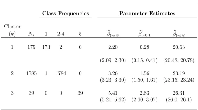
TABLE 3.2: Summary of Stage 2 clusters from simulation case 1. Parameter estimates are the posterior means and 95% credible intervals within each cluster. The table omits one singleton cluster consisting of a subject from Class 2. Clusters are ordered by the magnitude of their parameter estimates.
Class Frequencies Parameter Estimates
Cluster
(k) Nk 1 2-4 5 βb(∗k)0 βb(∗k)1 βb(∗k)2
1 175 173 2 0 2.20 0.28 20.63
(2.09, 2.30) (0.15, 0.41) (20.48, 20.78)
2 1785 1 1784 0 3.26 1.56 23.19
(3.23, 3.30) (1.50, 1.61) (23.15, 23.24)
3 39 0 0 39 5.41 2.83 26.31
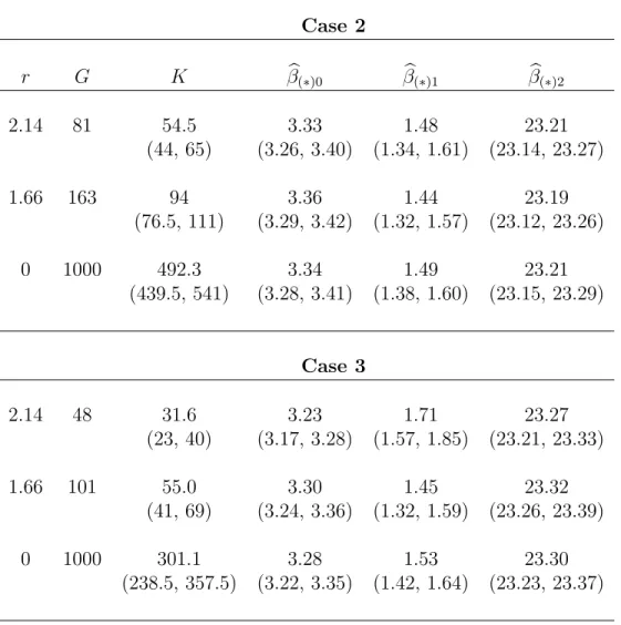
TABLE 3.3: Means and 95% credible intervals forK and βb(∗) from simulation cases 2
and 3. The true values of the population effects were approximatelyβ= (3.3,1.5,23.2)0 in each case.
Case 2
r G K βb(∗)0 βb(∗)1 βb(∗)2
2.14 81 54.5 3.33 1.48 23.21
(44, 65) (3.26, 3.40) (1.34, 1.61) (23.14, 23.27)
1.66 163 94 3.36 1.44 23.19
(76.5, 111) (3.29, 3.42) (1.32, 1.57) (23.12, 23.26)
0 1000 492.3 3.34 1.49 23.21
(439.5, 541) (3.28, 3.41) (1.38, 1.60) (23.15, 23.29)
Case 3
2.14 48 31.6 3.23 1.71 23.27
(23, 40) (3.17, 3.28) (1.57, 1.85) (23.21, 23.33)
1.66 101 55.0 3.30 1.45 23.32
(41, 69) (3.24, 3.36) (1.32, 1.59) (23.26, 23.39)
0 1000 301.1 3.28 1.53 23.30
smoker (N1 = 6,684), ex-smoker (N2 = 1,849), or current smoker (N3 = 8,985). In
Stage 1, we stratified by exposure and the four most common missingness patterns: no missing data, missing followup at year 8, missing followups at years 3 and 8, and lost to followup following year 1. Within each stratum, we clustered under r = 2.14(pj/6)1/2
wherepj is the number of followups under the missingness pattern in stratum j. Note
that the correction, (pj/6)1/2, is the reciprocal of the correction used in (3.5). These
Stage 1 analyses generatedG= 526 clusters across the 12 strata.
In Stage 2, we modelled the weight of pseudo-subject g using an intercept, x∗g0, indicators of smoking exposure (x∗g1 for ex-smokers andx∗g2 for current smokers), mean age at each followup (x∗g3), and ex-smoker by age (x∗g4) and current smoker by age (x∗g5) interactions. Age was centered around the mean value amongst the pseudo-subjects (3.16) and was assumed to have a linear effect due to the relatively few ages at which measurements were collected.
We used the same priors for τ, µ, and D as in the simulations and assigned a Ga(0.5,1) to α to express an a priori belief in few second stage clusters. We ran our MCMC for 45,000 iterations following a burn-in of 10,000, otherwise implementing as in Section 4.
3.5.2
Results
As in Chen et al. (2006), our estimated population effects suggest that a mother’s smoking habits during pregnancy had a significant impact on the growth of female chil-dren. As seen in Table 3.4, the 95% credible intervals for the smoking-age interactions (β4 and β5) obtained using our method (denotedG-DPP) are above 0, suggesting that
the effects of smoking on child weight increased with age. To describe the smoking effect, we provide estimates of the ex-smoker and current smoker effects at birth (ηE0
and ηC0) and age 8 (ηE8 and ηC8). At birth, the children of ex-smokers and current
smokers were leaner than the children of never smokers, with the decrease being highly significant, Pr(ηC0 < 0) and Pr(ηE0 < 0) > 0.99, but similar across the two groups,
Pr(ηC0 < ηE0)=0.668. However, at age 8, children in both exposure groups were
sig-nificantly heavier, Pr(ηC0 > 8) and Pr(ηE8 > 0) > 0.999, with the increase in weight
being greater in the children of ex-smokers, Pr(ηE0 > ηC8) = 0.997. It is likely that
did persist following adjustment for confounders.
Table 3.4 also presents smoking effect estimates obtained using GEE as in Chen et al.’s (2005) covariate adjusted models. Although the GEE estimates suggest a sig-nificant effect of smoking on child weight, there is no sigsig-nificant ex-smoker by age interaction (p = 0.141). It is not surprising that GEE provides a flatter slope for the ex-smoker effect since, under the assumption of MCAR, it does not allow a child’s ob-served weight to be related to her missingness pattern, which, as discussed in Section 2, appears to be the case in the CPP.
Another common method for large data sets is to fit a model to a random sub-sample of the data. Thus, we compared our population effect estimates to those obtained from fitting a semiparametric random effects model to two random samples of size 1752 (denoted RS1-DPP and RS2-DPP in Table 3.4). In each case, the ex-smoker effects had wide credible intervals and were insignificant. However, the results for the current smoker effects were not consistent across the random samples; in one sample the effect increased with age, while in the other sample, the effect was insignificant. These results demonstrate two key weaknesses of fitting a model to a random sample: a loss of power to detect an effect of a rare exposure and, since the method is sensitive to outliers in the data, dependence on the sample chosen. Our method does not suffer from either weakness since we preserve all scientifically important differences in Stage 1 and, by weighting our population effects by cluster size, we ensure that our estimates are re-flective of the complete data. The two-stage methodology is also more computationally efficient; in this example it took approximately 30 more hours to complete the MCMC for RS1- and RS2-DPP.
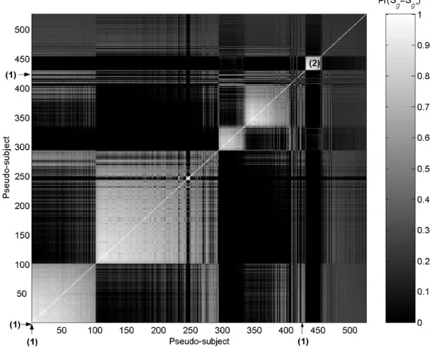
Figure 3.2 summarizes the Dirichlet process clustering of the pseudo-subjects in Stage 2. Although the posterior mean and 95% credible interval for K were 10.2 (6, 17), the clustering probabilities, i.e. Pr(Sg =Sg∗), indicate that many of these Stage 2
the iterations. Although some of these subjects appear to be outliers with unusual growth patterns, most (1,722) were lost to follow-up following birth or year 1 and the DPP could not accurately classify them due to their limited data. Had we not stratified by missingness in Stage 1, it is likely that many of these subjects would be grouped with the normal subjects. However, we discourage this practice as it increases the amount of imputation in the Stage 1 clusters.
3.6
Discussion
We have proposed a two-stage clustering procedure for fitting Bayesian semiparamet-ric random effects models to large data sets. Our method uses expert elicitation to generate a smaller, biologically meaningful, pseudo-sample of data that summarize the important differences in the complete data. Then, by applying the DPP to these data, we substantially decrease the computational burden and generate scientifically inter-esting clusters in the posterior. Simulation studies have shown that our method can detect true trends in the data under discrete and continuous random effects, though there may be a small bias for multimodal, continuous distributions.
In applying our method to the CPP data, we have provided the first random effects analysis of the smoking data. Although our overall conclusions on the effect of maternal smoking during pregnancy are similar to those in Chen et al. (2006), we have also shown that their GEE methodology may have underestimated the effects of smoking on child weight. Our semiparametric method also allows inferences on heterogeneity in the smoking effects as well as the identification of clusters of subjects with large regression coefficients. Some of these outliers could be explained by confounders that were omitted from our model, such as maternal weight. Others likely reflect data entry or recording errors, and thus, an attractive feature of our approach is that inferences on subjects in the larger clusters are not sensitive to these outliers.
FIGURE 3.2: Dirichlet process clustering of CPP data. The order of the pseudo-subjects corresponds to the order of the singleton clusters in a dendrogram generated in Matlab (version 6). This dendrogram summarized nearest-neighbors clustering of the pseudo subjects using 1-Pr(Sg =Sg∗) as the distance measure. The arrows denote
CHAPTER 4
BAYESIAN SEMIPARAMETRIC
DYNAMIC FRAILTY MODELS
FOR MULTIPLE EVENT TIME
DATA
4.1
Introduction
Many biomedical studies are designed to assess covariate effects on the time to recur-rence of health-related outcomes, such as infections, hospitalizations, or recurrecur-rences of disease. For example, data of this type are collected in chemoprevention and car-cinogenicity studies measuring the rate of appearance of palpable tumors of the skin and breast of mice (Gail et al., 1980; Forbes and Sambuco, 1998; Dunson, 2000). In these experiments, a rich set of data are available for each mouse, including times of appearance of each lesion, total number of tumors, and time of death.
occur-ring with age result in complex and unanticipated trends in susceptibility to tumor development. A likely trend is that animals getting tumors relatively early may not be at higher risk later in life.
Recently, several authors have proposed more flexible, dynamic formulations. Yue and Chan (1997) and Yau and McGilchrist (1998) introduced a proportional hazard model for inter-recurrence times in which a subject’s frailty changes following each event, and Lam et al. (2002) developed a related approach for the proportional odds model. In tumorigenicity studies, a time-varying frailty structure may be more realistic since it is more natural to model individual-specific risk as changing with age instead of according to previous occurrences of tumors. Relevant methods have been proposed by Henderson and Shimakura (2003), who developed a longitudinal Poisson regression model with gamma frailties which vary with time, and Paik et al. (1994), who proposed a proportional hazards frailty model with a time-specific random factor. Although promising, these methods involve complicated likelihoods and difficult computation, particularly when one considers generalizations (e.g., for joint modelling).
Bayesian approaches have several advantages for data collected from tumorigenicity studies, including ease of computation via MCMC, ability to incorporate prior infor-mation (e.g., from historical controls), and exact inferences on different aspects of the tumor response (time to first tumor, total tumor burden, etc). Unfortunately, in the Bayesian literature there has been limited consideration of dynamic frailty models and methods for multiple event time data in general. For recent Bayesian references on frailty models for multiple event time and multivariate survival data, refer to pa-pers by Gustafson (1997), Sahu et al. (1997), Walker and Mallick (1997), Sargent (1998), Aslanidou et al. (1998), Sinha (1998), Chen and Sinha (2002), Dunson and Chen (2004), Sinha and Maiti (2004)), as well as a review in Ibrahim et al. (2001). H¨ark¨anen et al. (2003) proposed an innovative approach based on a model that al-lows subject-specific frailty trajectories to vary according to a latent class structure. In many settings, including animal tumorigenicity studies, it may be more natural to suppose that the age-specific risk trajectories vary according to a continuum, with each subject potentially having their own unique pattern.