Full Terms & Conditions of access and use can be found at
https://www.tandfonline.com/action/journalInformation?journalCode=hmbr20
Multivariate Behavioral Research
ISSN: 0027-3171 (Print) 1532-7906 (Online) Journal homepage: https://www.tandfonline.com/loi/hmbr20
The Analysis of Multivariate Longitudinal Data: An
Instructive Application of the Longitudinal
Three-Mode Three-Model
M. G. E. Verdam & F. J. Oort
To cite this article: M. G. E. Verdam & F. J. Oort (2019) The Analysis of Multivariate Longitudinal Data: An Instructive Application of the Longitudinal Three-Mode Model, Multivariate Behavioral Research, 54:4, 457-474, DOI: 10.1080/00273171.2018.1520072
To link to this article: https://doi.org/10.1080/00273171.2018.1520072
© 2019 The Author(s). Published by Informa UK Limited, trading as Taylor & Francis Group
Published online: 11 Mar 2019.
Submit your article to this journal
Article views: 1068
View related articles
The Analysis of Multivariate Longitudinal Data: An Instructive Application
of the Longitudinal Three-Mode Model
M. G. E. Verdama,band F. J. Oorta,b a
Department of Medical Psychology, Academic Medical Centre University of Amsterdam, Amsterdam, The Netherlands;bResearch Institute Child Development and Education, University of Amsterdam, Amsterdam, The Netherlands
ABSTRACT
Structural equation modeling is a common technique to assess change in longitudinal designs. However, these models can become of unmanageable size with many measure-ment occasions. One solution is the imposition of Kronecker product restrictions to model the multivariate longitudinal structure of the data. The resulting longitudinal three-mode models (L3MMs) are very parsimonious and have attractive interpretation. This paper provides an instructive description of L3MMs. The models are applied to health-related quality of life (HRQL) data obtained from 682 patients with painful bone metastasis, with eight measurements at 13 occasions; before and every week after treat-ment with radiotherapy. We explain (1) how the imposition of Kronecker product restric-tions can be used to model the multivariate longitudinal structure of the data, (2) how to interpret the Kronecker product restrictions and the resulting L3MM parameters, and (3) how to test substantive hypotheses in L3MMs. In addition, we discuss the challenges for the evaluation of (differences in) fit of these complex and parsimonious models. The L3MM restrictions lead to parsimonious models and provide insight in the change pat-terns of relationships between variables in addition to the general patpat-terns of change. The L3MM thus provides a convenient model for multivariate longitudinal data, as it not only facilitates the analysis of complex longitudinal data but also the substantive inter-pretation of the dynamics of change.
KEYWORDS Kronecker product; longitudinal factor model (LFM); longitudinal three-mode model (L3MM); multivariate
longitudinal data
Introduction
Longitudinal studies in the life-sciences involve mul-tiple observations at mulmul-tiple measurement occasions, yielding multivariate longitudinal data sets. Structural equation modeling (SEM) offers a general and versa-tile framework for the analysis of such data. Compared with usual regression methods, SEM allows for the use of latent variables and measurement error of observed variables, and provides tests for overall goodness of fit, for specific hypotheses about relation-ships between variables and about longitudinal devel-opment. The longitudinal factor model (LFM; Oort,
2001; Tisak & Meredith, 1990) may include multiple latent variables, with multiple indicators from multiple measurement occasions, and thus enables investigation of complex longitudinal relations. However, the LFM becomes progressively large and unmanageable when
the number of measurement occasions increases. One of the methods that facilitates the investigation of lon-gitudinal relations in more extensive data structures is the so-called longitudinal three-mode model (L3MM; Oort, 2001). In this paper, we provide an instructive description of the L3MM and illustrate how it can be used to test substantive hypotheses. It is our aim to facilitate applications of L3MMs for the investigation and interpretation of longitudinal dynamics, and thus help researchers and practitioners who are interested in developmental processes. In order to fully profit from the current tutorial, we recommend that the reader is familiar with the general SEM framework (cf. Bollen, 1989) and the LFM in particular.
The increased complexity of multivariate longitu-dinal data with larger numbers of measurement occa-sions can be best illustrated with an example. Imagine that we want to study the development of three
CONTACT M. G. E. Verdam [email protected] Department of Child Development and Education, University of Amsterdam, PO Box 15776, 1001 NG Amsterdam, The Netherlands.
Supplemental data for this article can be accessedhere.
ß2019 The Author(s). Published by Informa UK Limited, trading as Taylor & Francis Group
This is an Open Access article distributed under the terms of the Creative Commons Attribution-NonCommercial-NoDerivatives License ( http://creativecommons.org/licenses/by-nc-nd/4.0/), which permits non-commercial re-use, distribution, and reproduction in any medium, provided the original work is properly cited, and is not altered, transformed, or built upon in any way.
2019, VOL. 54, NO. 4, 457–474
constructs measured with three indicator variables each, which yields a data-structure consisting of nine indicators and three common factors. The LFM requires estimation of 78 parameters when it includes two measurement occasions, 228 parameters when it includes four measurement occasions, and 450 param-eters when it includes six measurement occasions (see Appendix A for the calculation of the numbers of parameters). Estimation of model parameters may be difficult with such large models. Also, it has been argued that the trustworthiness of results decreases when the number of parameter estimates increases in relation to the sample size (Bentler & Chou, 1987; Jackson, 2003; Kline, 2011). Although the trustworthi-ness of results may also depend on many other model characteristics such as the number of variables per factor and the values of the factor loadings (Gagne & Hancock, 2006; Marsh, Hau, Balla, & Grayson, 1998), it seems plausible that convergence of estimation and stability of parameter estimates will be negatively affected with increasing model size because of increas-ing numbers of measurement occasions. More import-antly, it becomes more difficult to arrive at a meaningful interpretation of findings when the num-ber of model parameters is larger. For the interpret-ation of relinterpret-ations between the common factors from 2, 4, or 6 measurement occasions in the situation above, the LFM yields 15, 66, or 153 common factor covariances, respectively (see Appendix A). Such large numbers of parameter estimates complicate a mean-ingful interpretation of change in the relationships between common factors across time.
The increasing complexity of multivariate longitu-dinal models with multiple measurement occasions can be reduced by imposing additional restrictions on model parameters. Three-mode models are suited for the analysis of sets of data that are characterized by three modes. Multivariate longitudinal data are a kind of three-mode data, with the modes referring to the subjects, the variables, and the measurement occasions. Principal component and factor analysis techniques for three-mode data originate from Tucker’s (1966) three-mode principal component analysis (e.g., the Tucker3 model), and include extensions of component analyses (e.g., the Candecomp/Parafac model; Carroll & Chang, 1970; Harshman, 1970), and of common factor analysis (Bentler & Lee, 1979; Bentler, Poon, & Lee, 1988; Bloxom, 1968). In the present paper, we focus on three-mode common factor analysis (see Kiers & van Mechelen, 2001; Smilde, Bro, & Geladi, 2004; Kroonenberg, 2008 for more general overviews of
three-mode methods). The advantage of the com-mon factor analysis framework is that it incorpo-rates a versatile range of models and hypotheses to be tested. In addition, factor analysis techniques for multivariate longitudinal data are a special topic, as they offer unique opportunities for modeling the three-mode structure of the data (Oort, 1999) that not only greatly improve model parsimony but also facilitate interpretation of model parameters.
multiplicative structure similar to longitudinal struc-tures such as compound symmetry, autoregressive or latent curve models, which are often described as con-venient models to simplify the correlation matrix of repeated measures (cf. Crowder & Hand, 1990; Lindsey,1993). However, if the underlying assumption of the proposed Kronecker product restrictions does not hold, this may lead to biased estimates of effects. With the L3MM, the tenability of the Kronecker product restrictions can be tested, but the evaluation of (differences in) model fit is complicated due to the size of the models and increased parsimony of L3MMs. In the current tutorial, we will, therefore, also address the challenges of how to make appropri-ate decisions in evaluating the imposed L3MM restric-tions, by using a combination of model fit statistics and substantive considerations.
The main benefit of increased model parsimony is that it enables the analysis of multivariate longitu-dinal data from many measurement occasions within the general SEM framework. Equally important, however, is that the substantive interpretation of changes in the relations between variables is facili-tated as the L3MM yields separate estimates for the relationships between (observed and latent) variables and the relationships between the measurement occasions (i.e., the change in the relationships between the variables over time). The L3MM thus has the potential to improve our insight of longitu-dinal dynamics in the life sciences in general, and is especially suited to investigate and test the nature of these dynamics in multiple behavioral, cognitive, or psychophysiological measures (e.g., how the relation-ships between different neurological functionalities change with age, whether the variability in different mental abilities changes proportionally over time, or how the strength between several health outcomes is affected by therapeutic intervention). However, as of yet only few applications exist in the literature that take advantage of these unique characteristics of the L3MM. That is, applications are mostly limited to (technical) explanations (Kroonenberg & Oort, 2003; Oort,2001) and are not yet used to address substan-tive research questions. There is thus a need to bridge the gap between the availability of L3MM model strategies for the analyses of longitudinal dynamics and their application.
The aim of the present paper is to provide an instructive description of L3MMs in order to stimulate their successful application. First, we will explain (1) how the imposition of Kronecker product restrictions can be used to take into account the multivariate
longitudinal structure of the data, (2) how to interpret the Kronecker product restrictions and the resulting L3MM parameters, and (3) how to test substantive hypotheses in L3MMs. Second, we will illustrate the application of L3MMs with an example of health-related quality of life (HRQL) data obtained from 682 patients with painful bone metastasis, with eight measurements at 13 occasions (104 variables); before and every week after treatment with radiotherapy. Part of these data have been analyzed before using simple repeated measures analyses to compare the development of HRQL between two different treat-ment regimens (Steenland et al., 1999), or using between group analyses to compare scores from only one specific measurement occasion (van der Linden et al., 2004). The latent variable model enables the analysis of changes in HRQL in much more detail, as it not only provides insight into changes in the means of variables, but also in changes in relations between variables over time. Using the example of bone meta-stases, we will illustrate how the L3MM can be suc-cessfully applied to provide a more comprehensive analysis of the multivariate longitudinal development of HRQL.
The L3MM
In order to facilitate the explanation of the L3MM, we will first describe the longitudinal factor model (LFM) and show how Kronecker product restrictions can be applied to yield the L3MM. Suppose R latent traits are measured with K observed variables on J occasions, the means and covariances of the observed variables are given by
Eð Þ ¼x l¼sþKj; (1)
and
Covðx;x0Þ ¼R¼KUK0þH; (2)
where s is a JK-vector of intercepts, K is a JKJR
matrix of common factor loadings, jis a JR-vector of common factor means, U is a JRJR symmetric matrix containing the variances and covariances of the common factors, and H is aJKJK symmetric matrix containing the variances and covariances of the residual factors. To achieve identification of all model parame-ters, scales and origins of the common factors can be established by fixing the intercept of one indicator per common factor (e.g., at zero), and fixing one common factor loading per common factor (e.g., at one).
these restrictions on each of the parameter matrices, and show how further restrictions can be imposed to test substantive hypotheses. Specifically, we will explain the imposition of Kronecker product restric-tions on (1) factor loadings and intercepts (K and s) to comply with longitudinal measurement invariance; (2) residual factor variances and covariances (H), and additional restrictions to test equality of variances, correlations and covariances across occasions; (3) common factor variances and covariances (U), and additional restrictions to test equality of variances, correlations and covariances across occasions; and (4) common factor means (j), and additional restrictions to test a linear trend of common factor means. This sequence of imposing Kronecker product restrictions was chosen because the K and s restrictions (1) are the most logical starting point from the researcher’s perspective, as longitudinal measurement invariance is required for the comparison of common factors means, the H and U restrictions (2, 3) are most effective in increasing model parsimony and facilitat-ing parameter interpretation, while j imposed restric-tions (4) can be used to test specific hypotheses regarding the common factor means while profiting from the model parsimony yielded by the earlier restrictions.
Longitudinal measurement invariance
With longitudinal data, the structure of matrix K is a block diagonal matrix containing matrices of factor loadings of each measurement occasion on the diagonal (K1, K2, …, Kj, …, KJ; see Table 1), where each of the Kj is aKR matrix containing the factor loadings of occasion j. Vector s consists of stacked vectors of
intercepts from all measurement occasions (s1, s2, …,
sj, …,sJ;seeTable 1), where each of thesjis of length
K. To test substantive hypotheses about the common factors, it is required that the meaning of these factors is the same across occasions. The requirement of longi-tudinal measurement invariance entails that the com-mon factor loadings (Kj) and the intercepts (sj) are invariant across occasions (i.e., Kj¼K0, and sj¼s0 for all j). The usual longitudinal measurement invariance restrictions, that is, equality restrictions on factor load-ings and intercepts across time, can be written as a Kronecker product constraint:
K¼IK0; (3)
s¼us0; (4)
whereK0is aKRmatrix of invariant common factor loadings,s0 is a K-vector of invariant intercepts,I is a
JJ identity matrix, u is a J-vector of ones, and the symboldenotes the Kronecker product (seeTable 1). The Kronecker product is an operation that can be applied to two matrices A andB of arbitrary size, and results in a block matrix that contains the matrices B pre-multiplied by each element ofA(see Appendix B). The Kronecker product operations in Eqs. (3) and (4)
impose the restriction that factor loadingsK0and inter-ceptss0apply to all measurement occasions.
Residual factor variances and covariances
Matrix H is a symmetricJKJK matrix, consisting of
KKHjj’matrices that contain the covariances of the
residual factors on occasion j with the residual factors on occasion j’. Residual factors do not correlate with other residual factors, but are allowed to correlate with the same residual factors across occasions. Thus,
Table 1. Imposition of measurement invariance restrictions on factor loadings and intercepts using the Kronecker product.
Factor loadings (K5IK0), assumingKj¼K0for allj
K(JKxJR) I(JxJ) K0(KxR)
K1ðKxRÞ
K2 K3 ::: KJ 5 1 1 1 ::: 1
k11 ::: k1R k21 ::: k2R k31 ::: k3R
::: ::: :::
kK1 ::: kKR
Intercepts (s5us0), assumingsj¼s0for allj
s(JKx1) u(Jx1) s0(Kx1)
s1ðKx1Þ
s2 s3 ::: sJ ¼ 1 1 1 ::: 1 s1 s2 s3 ::: sK
Notes:K0ands0contain invariant factor loadings and intercepts of one measurement occasion that are applicable to all measurement occasions,Iandu
all Hjj’ matrices are diagonal. Imposition of the Kronecker product restriction entails
H¼HTHV; (5)
where the full JKJK matrix (H) is decomposed into two smaller matrices that describe the relations between the measurement occasions (HT; a symmetric matrix of dimensions JJ) and the variances of the residual factors (HV is a diagonal matrix of dimen-sions KK, containing within occasion correlations between residual factors) (see Table 2). The subscripts
“T”and “V”refer to “time”and“variable.” To achieve identification at least one parameter of HT or HV needs to be fixed at a non-zero value. Fixing the first element of HT to unity is a convenient choice for the interpretation of parameter estimates. MatrixHV then contains the residual factor variances at the first meas-urement occasion, and HT contains the relationships between residual factors across time that apply to all residual factors. We refer to these estimates as coeffi-cients of proportionate change. If useful, matrix HT can be further restricted to conform to, for example, compound symmetry, autoregressive, or latent curve structures (Oort,2001). Imposing the Kronecker prod-uct restriction implies that the changes in variances and covariances of the residual factors across occa-sions are proportionate for all residual factors.
To further facilitate interpretation of parameter estimates it is convenient to use a reparameterization that decomposes the residual factor variances and covariances of H into correlations H* and standard deviationsD:
H¼DHD; (6)
where D is a JKJK diagonal matrix containing the standard deviations of the residual factors, and diag(H*)¼I, so that the off-diagonal elements of H* contain the correlations between the residual factors. This, in turn, enables the imposition of Kronecker product restrictions on residual factor correlations, using
H¼HTHV; (7)
where the full correlation matrix (H*) is decomposed into two smaller matrices that describe the correla-tions between the measurement occasions (HT*) and the correlations between residual factors (HV*). As residual factors do not correlate with other residual factors, HV*¼I (seeTable 2). The reparameterization, therefore, allows investigation of the Kronecker prod-uct restrictions on residual factor correlations, while allowing each residual factor to have a unique stand-ard deviation.
In addition, Kronecker product restrictions can be imposed on the standard deviations of the residual factors, using
D¼DTDV; (8)
where DT is a JJ diagonal matrix that describes the proportionate change in standard deviations across occasions, and DV is a diagonal KK matrix that contains the standard deviations of the residual factors at the first occasion (see Table 2). Imposition of Kronecker product restrictions on both H* and D is equivalent to the imposition of the Kronecker product restriction directly on H(as in Eq. (5)).
Table 2. Imposition of Kronecker product restrictions on residual factor variances and covariances.
Residual factor variances and covariances (H¼HTHV)
H(JKxJK) HT(JxJ) HV(KxK)
H11ðKxKÞ
H21 H22
::: ::: :::
HJ1 HJ2 ::: HJJ
5 hhT11T21 hT22
::: ::: :::
hTJ1 hTJ2 ::: hTJJ
hV11 hV22
::: hVKK
Residual factor correlations (H*¼HT*HV*)
H*(JKxJK) HT*(JxJ) HV*(KxK)
IðKxKÞ H
21 I
::: ::: :::
H
J1 HJ2 ::: I
5 1hT21 1
::: ::: :::
hTJ1 hTJ2 ::: 1
1 1 ::: 1
Residual factor standard deviations (D¼DTDV)
D(JKxJK) DT(JxJ) DV(KxK)
D1ðKxKÞ
D2 ::: DJ
5 dT11 dT22
::: dTJJ
dV11 dV22
::: dVJJ
Notes: Residual factor covariances (H), correlations (H*), and standard deviations (D) are decomposed using the Kronecker product (), whereHT,HT*,
andDTrepresent relationships between measurement occasions of residual factor covariances, correlations, and standard deviations, respectively; and
Substantive hypotheses: Further restrictions enable hypothesis tests about the equality of residual factor correlations, variances, and covariances.
Equality of residual factor correlations of the same lag is investigated by imposing a banded structure on
HT* in Eq. (7) so that all elements of the same
diag-onal are equal. This restriction implies that correla-tions between residual factors at the first occasion and residual factors at the second occasion are equal to correlations between residual factors at the second and third occasion, and so on.
Equality of residual factor standard deviations is investigated by imposing:
D¼ID0; (9)
where I is a JJ identity matrix and D0 contains the invariant standard deviations of the residual factors of one measurement occasion that are applicable to all measurement occasions.
Equality of residual factor covariances across occasions of the same lag is tested by imposing both restrictions described above. This is equivalent to the imposition of the Kronecker product to H (as in
Eq. (5)), where the banded structure is imposed
on HT.
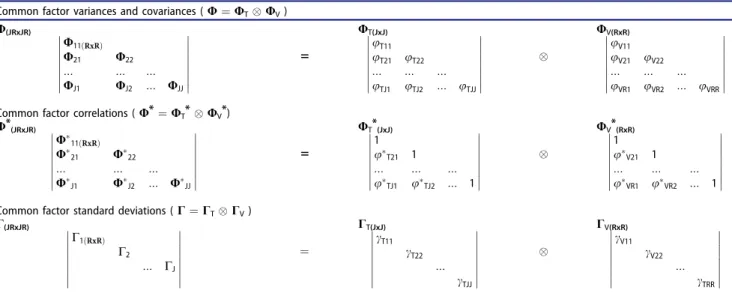
Common factor variances and covariances
The procedure of imposing Kronecker product restric-tions on the matrix of common factor variances and covariances is largely similar to the procedure for imposing Kronecker product restrictions on the
matrix of residual factor variances and covariances described above.
Matrix U is a JRJR symmetric matrix, consisting of RR Ujj’ matrices that contain the covariances of the common factors at occasion j with the common factors at occasion j’. Imposition of the Kronecker product restriction implies that the change in relations between the common factors across occasions is pro-portionate for all common factors1:
U¼UTUV; (10)
whereUTis aJJsymmetric matrix that describes the relationships between the measurement occasions, and
UVis aRRsymmetric matrix that describes the rela-tionships between the variables (see Table 3). For the purpose of identification, the first element ofUTcan be fixed at unity so that UV contains the common factor variances and covariances at the first measurement occasion, andUTcontains coefficients of proportionate change. If useful, matrixUTcan be further restricted to conform to, for example, compound symmetry, autore-gressive, or latent curve structures (Oort,2001).
In addition, it is convenient to use the following reparameterization:
U¼CUC; (11)
where C is a JRJR diagonal matrix containing the standard deviations of the common factors, and
Table 3. Imposition of Kronecker product restrictions on common factor variances and covariances.
Common factor variances and covariances (U¼UTUV)
U(JRxJR) UT(JxJ) UV(RxR)
U11ðRxRÞ
U21 U22
::: ::: :::
UJ1 UJ2 ::: UJJ
5 uuT11T21 uT22
::: ::: :::
uTJ1 uTJ2 ::: uTJJ
uuV11V21 uV22
::: ::: :::
uVR1 uVR2 ::: uVRR
Common factor correlations (U*¼UT*UV*)
U*
(JRxJR) UT*(JxJ) UV*(RxR)
U
11ðRxRÞ
U
21 U22
::: ::: :::
U
J1 UJ2 ::: UJJ
5 1uT21 1
::: ::: :::
uTJ1 uTJ2 ::: 1
1uV21 1
::: ::: :::
uVR1 uVR2 ::: 1
Common factor standard deviations (C¼CTCV)
C(JRxJR) CT(JxJ) CV(RxR)
C1ðRxRÞ
C2
::: CJ
¼ cT11 cT22
::: cTJJ
cV11 cV22
::: cTRR
Notes: Common factor covariances (U), correlations (U*) and standard deviations (C) are decomposed using the Kronecker product (), whereUT,UT*,
andCTrepresent relationships between measurement occasions of common factor covariances, correlations, and standard deviations, respectively; and
UV,UV*,andCVrepresent common factor variances, correlations, and standard deviations of one measurement occasion, respectively.
1
We note that the Kronecker product restriction of Eq. (10) is equivalent to a second order factor modelU¼K2UTK2’ in whichK2contains the
factor loadings of the (first-order) common factors on the second-order common factors, invariant across occasions (K25I(JxJ) k(Rx1) so that
diag(U*)¼I so that all off-diagonal elements of U* are correlations between the common factors. This, in turn, allows for imposition of the Kronecker product restriction on the correlations between common fac-tors (U*) and the common factor standard deviations (C) separately
U¼UTUV; (12)
and
C¼CTCV; (13)
whereUT* contains the correlations between measure-ment occasions, UV* contains the correlations between common factors irrespective of the measure-ment occasions, CT contains coefficients of propor-tionate change in standard deviations across occasions (where the first element of CT is fixed to unity for identification), and CV contains the standard devia-tions of the common factors at the first measurement occasion (seeTable 3). Imposition of Kronecker prod-uct restrictions on both U* andC is equivalent to the imposition of the Kronecker product restriction dir-ectly toU.
Substantive hypotheses: Equality of common factor
variances, correlations and covariances across occa-sions can be tested by further restricting the L3MM matrices.
The hypothesis of equal common factor correla-tions across occasions of the same lag is investigated by imposing a banded structure onUT* inEq. (12) so that all elements of the same diagonal are equal. Because UV* is a symmetric matrix, this restriction entails that both the correlations between the common
factors of one measurement occasion are equal across occasions, and that correlations between common fac-tors at the first and second measurement occasions are equal to correlations between common factors at the second and third measurement occasions, and so on.
The hypothesis of equality of common factor var-iances across occasions is investigated by imposing
C¼IC0; (14)
where I is a JJ identity matrix and C0 is an RR matrix that contains the invariant standard deviations of the common factors of one measurement occasion that apply to all measurement occasions.
Equality of common factor covariances across occa-sions of the same lag is tested by imposing both restrictions described above, which is equivalent to imposing a banded structure directly on UT in
Eq. (10).
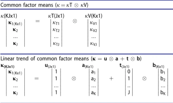
Common factor means
The JR-vector j consists of stacked jj vectors of
length R, containing the common factor means of occasion j. The imposition of the Kronecker product restriction requires only estimation ofjT andjV:
j¼jTjV; (15)
where jT is the J-vector that contains coefficients of proportionate change in common factor means across occasions, and jV is aR-vector that contains the com-mon factor means at the first measurement occasion
(seeTable 4).
Substantive hypotheses: To test and facilitate
inter-pretation of (possible) changes in common factor means across time, we may impose various restric-tions on j. For example, to test for linear develop-ment of common factor means, we can impose
j¼uaþtb; (16)
where u is a unity J-vector, a is a K-vector of inter-cepts, t is a J-vector with some coding for the time of the occasions (for example 0, 1, 2, … J), and b is a
K-vector of slope parameters (see Table 4). The slope parameters then give an indication of the change across time for each common factor (instead of hav-ing to interpret all separate estimates of common fac-tor means). To test invariance of common facfac-tor means we can fix the slopes at zero (i.e., b¼0).
Table 4. Imposition of Kronecker product restrictions on com-mon factor means.
Common factor means (j¼jTjV)
j(KJx1) jT(Jx1) jV(Kx1) j1ðKx1Þ
j2 ::: jJ
¼ jT1
jT2 ::: jTJ jV1 jV2 ::: jVJ
Linear trend of common factor means (j¼uaþtb) j(KJx1) u(Jx1) a(Kx1) t(Jx1) b(Kx1)
j1ðKx1Þ
j2 ::: jJ
¼ 11
::: 1
aa12
::: aK
þ 01
:: J
bb12
::: bK
Notes: Common factor means (j) are decomposed using the Kronecker product (), where jT represents relationships between measurement
occasions, jVrepresents common factor means of one measurement
Longitudinal structures of common factor
To further test substantive hypotheses regarding the common factors, one can apply longitudinal structures to both the covariance and mean structures of the common factors. Examples of these longitudinal struc-tures are the autoregressive model and the latent curve model, which are common extensions within the SEM framework. For an explanation of these models, including possible variations and examples of hypotheses testing, the reader is referred to Oort (2001).
Illustrative example
Sample
The sample in the current study is a subset from the sample from the Dutch Bone Metastasis Study (DBMS; Steenland et al., 1999; van der Linden et al.,
2004, 2006). In the DBMS, a total of 1157 patients (533 women) with painful bone metastases from a solid tumor were enrolled from 17 radiotherapy insti-tutes in The Netherlands. The purpose of the study was to investigate the effectiveness of single fraction
versus multiple fraction radiation therapy for patients with painful bone metastases; the primary endpoint of the study was response to pain. The Medical Ethics Committees of all participating institutions approved the study and all patients gave their informed consent. For the present study, only patients who survived at least 13 weeks were included, which resulted in a total sample size of 682 patients (354 women). Patients’ primary tumor was either breast cancer (n¼321), prostate cancer (n¼181), lung cancer (n¼106), or other (n¼74). Ages ranged from 33 to 90, with a mean of 64.2 (standard deviation 11.5).
Measures
Health-related quality of life questionnaires were administered before treatment (T0), and during the first 12 weeks of follow-up, patients completed weekly HRQL questionnaires by mail (T1 through T12). Questionnaire items were grouped into scales based on the results of principal component analysis of data from the first measurement occasion and substantive considerations (for more information see Verdam, Oort, van der Linden, & Sprangers, 2015). This resulted in the computation of eight health indicators: physical functioning (PF; four items), mobility (MB;
five items), social functioning (SF; two items), depres-sion (DP; eight items), listlessness (LS; six items), pain (PA; four items), sickness (SI; six items), and treat-ment-related symptoms (SY; 11 items). All scale scores were calculated as mean item scores, ranging from 1 to 4, with higher scores indicating more symp-toms or more dysfunctioning. Analysis at the scale level is consistent with the usual evaluation of the ori-ginal questionnaires that are still (partly) represented in the current scales, and was required to yield a manageable number of variables.
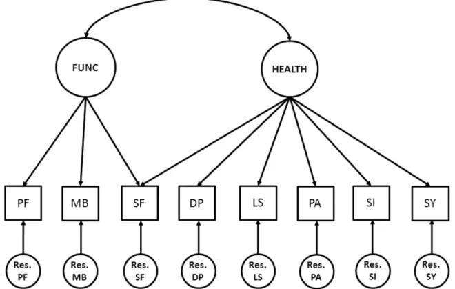
The eight health indicators were modeled to be reflective of two common factors: functional limita-tions and health impairments (see Figure 1). The squares represent observed variables (scale scores), the circles on the top represent the common factors, and the circles on the bottom represent residual factors. Functional limitations are measured by three observed variables, health impairments are measured by six observed variables, with one observed variable in common.
Statistical analyses
The programOpenMx(Boker et al.,2011) was used to run the statistical analyses. OpenMx is free and open source software for use within R that allows esti-mation of a wide variety of advanced multivariate statistical models. It was used because it allows for an operation of the structural equation model using matrix specifications, and therefore the Kronecker product restrictions can be easily applied. The vari-ance-covariance matrix and mean vector that were used for statistical analyses, and syntaxes of all analy-ses that are reported in this paper, are provided as onlineSupplementary material.
Evaluation of Goodness of Fit: To evaluate goodness
of fit the chi-square test of exact fit (CHISQ) was used, where a significant chi-square indicates a signifi-cant difference between model and data. As an alter-native, the root mean square error of approximation (RMSEA; Steiger, 1990; Steiger & Lind, 1980) was used as a measure of approximate fit, where an RMSEA value below .05 indicates “close” approximate fit, and values below .08 indicate “reasonable” approximate fit (Browne & Cudeck, 1992). Additionally, the expected cross-validation index (ECVI; Browne & Cudeck, 1989) can be used to com-pare different models for the same data, where the model with the smallest ECVI indicates the model with the best fit. The ECVI is linearly related to the Akaike Information Criteria (AIC; Akaike, 1987) and
thus provides the same ranking of competing models (Browne & Cudeck, 1992). However, the ECVI has the advantage that confidence intervals are available for the differences between ECVI values of nested models. For both the RMSEA and ECVI 95% confi-dence intervals were calculated using the program NIESEM (Dudgeon, 2003). We also calculated the Comparative Fit Index (CFI; Bentler, 1990), where the model of interest is compared to a model of independence, i.e., a model where all covariances in R are assumed zero. The CFI ranges from zero to one, and as a general rule of thumb values above 0.95 are indicative of relatively “good” model fit (Hu & Bentler, 1999).
With different tests and indices to evaluate model fit, providing decision rules on whether the fit of a model is “good” is complicated by the fact that one might find inconsistent results (e.g., a significant exact chi-square test, but close approximate fit according to the RMSEA). The researcher then has to make a deci-sion on which fit index is most appropriate for the data and hypotheses under study. For example, although the chi-square test of exact fit is the most commonly used, it is also generally acknowledged that it tends to become significant in larger samples and favors highly parameterized models. The described indices of approximate fit are less dependent on sam-ple size and reward model parsimony, but they usually do not provide a test of model fit. In our example of bone metastasis the sample size is large and the model has many degrees of freedom. As a result, the chi-square test of exact fit has high power to detect small, but clinically meaningless, differences between model and data. Therefore, in this paper, we will base our evaluation of overall model fit on indices of approxi-mate fit and will substantiate decisions on model fit evaluation in case of inconsistent results. A more extensive discussion about model fit evaluation follows in the discussion paragraph at the end of this paper (see also Verdam, 2017).
Evaluation of differences in Model Fit: To evaluate
differences between hierarchically related models the chi-square difference test (CHISQdiff) can be used,
where a significant chi-square indicates a significant difference in model fit. The ECVI difference (ECVIdiff) can be used to test equivalence in
approxi-mate model fit, where a value that is significantly larger than zero indicates that the more restricted model has significantly worse approximate fit. In add-ition, it has been proposed that the difference between CFI values (CFIdiff) can be used to evaluate
model fit between two nested models (Cheung & Rensvold, 2002). As a rule of thumb CFIdiff values
larger than 0.01 are taken to indicate that the more restricted model should be rejected. As confidence intervals are not available for CFI values, the CFIdiff
cannot be used to test whether the difference in model fit is significant.
Evaluation of differences in model fit is compli-cated for similar reasons as described above. When comparing different models for the same data, one has to decide on the tradeoff between a deterioration of model fit and a gain in model parsimony. Such decisions should be guided by the evaluation of differ-ences in model fit, but depend also on the substantive considerations with regard to interpretation of the model or model parameters. For example, the impos-ition of Kronecker product restrictions to take into account the multivariate longitudinal structure of the data generally leads to a large gain in model parsi-mony. When one considers the assumption of the multivariate structure of the data to be reasonable, one might not want to have too much power to detect
small, but trivial, differences between model and data. However, when testing specific substantive hypotheses, one might consider high power to detect small differ-ences to be beneficial. In this paper we will report results of all tests for differences in model fit that are explained above and will provide a rationale for the decision that is being made.
Results
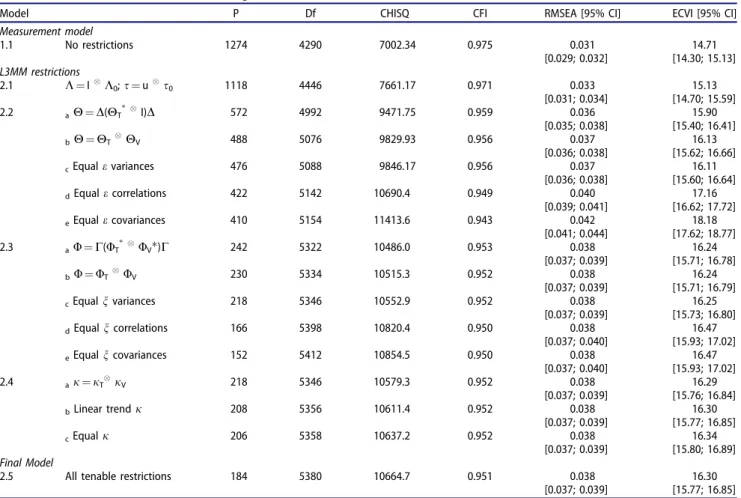
The measurement model of Figure 1was the basis for a structural equation model for baseline and follow-up measurements without any across occasion con-straints. This model yielded a chi-square test of exact fit that was significant but the RMSEA measure and CFI indicated close fit (see Table 5, Model 1.1). The number of model parameters to be estimated was 1274.
L3MMs were applied to the 104 variables from 13 measurement occasions to investigate change in HRQL. Kronecker product restrictions were imposed on (1) factor loadings and intercepts (K and s) to
Table 5. Goodness of overall fit of the longitudinal three-mode models.
Model P Df CHISQ CFI RMSEA [95% CI] ECVI [95% CI]
Measurement model
1.1 No restrictions 1274 4290 7002.34 0.975 0.031
[0.029; 0.032]
14.71 [14.30; 15.13] L3MM restrictions
2.1 K¼IK0;s¼us0 1118 4446 7661.17 0.971 0.033
[0.031; 0.034]
15.13 [14.70; 15.59]
2.2 aH¼D(HT I)D 572 4992 9471.75 0.959 0.036
[0.035; 0.038]
15.90 [15.40; 16.41]
bH¼HTHV 488 5076 9829.93 0.956 0.037
[0.036; 0.038]
16.13 [15.62; 16.66]
cEqualevariances 476 5088 9846.17 0.956 0.037
[0.036; 0.038]
16.11 [15.60; 16.64]
dEqualecorrelations 422 5142 10690.4 0.949 0.040
[0.039; 0.041]
17.16 [16.62; 17.72]
eEqualecovariances 410 5154 11413.6 0.943 0.042
[0.041; 0.044]
18.18 [17.62; 18.77]
2.3 aU¼C(UT UV)C 242 5322 10486.0 0.953 0.038
[0.037; 0.039]
16.24 [15.71; 16.78]
bU¼UTUV 230 5334 10515.3 0.952 0.038
[0.037; 0.039]
16.24 [15.71; 16.79]
cEqualnvariances 218 5346 10552.9 0.952 0.038
[0.037; 0.039]
16.25 [15.73; 16.80]
dEqualncorrelations 166 5398 10820.4 0.950 0.038
[0.037; 0.040]
16.47 [15.93; 17.02]
eEqualncovariances 152 5412 10854.5 0.950 0.038
[0.037; 0.040]
16.47 [15.93; 17.02]
2.4 aj¼jTjV 218 5346 10579.3 0.952 0.038
[0.037; 0.039]
16.29 [15.76; 16.84]
bLinear trendj 208 5356 10611.4 0.952 0.038
[0.037; 0.039]
16.30 [15.77; 16.85]
cEqualj 206 5358 10637.2 0.952 0.038
[0.037; 0.039]
16.34 [15.80; 16.89] Final Model
2.5 All tenable restrictions 184 5380 10664.7 0.951 0.038
[0.037; 0.039]
16.30 [15.77; 16.85]
comply with longitudinal measurement invariance; (2) residual factor variances and covariances (H), (3) common factor variances and covariances (U), and (4) common factor means (j). Substantive hypotheses were tested at each consecutive step. We illustrate the application of each of the L3MMs that were described above, and explain why each model could be of substantive interest.
Longitudinal measurement invariance: Longitudinal
measurement invariance is required in order to test substantive hypotheses about the common factors. The model with both factor loadings and intercepts restricted to be equal across occasions yielded a chi-square test of exact fit that was significant, but the RMSEA and CFI measures indicated close and good fit respectively (Model 2.1, see Table 5). To test whether the assumption of longitudinal measurement invariance holds, the model fit of this model can be compared to the model fit of the LFM without restrictions. Both the chi-square difference test and the ECVI difference test are significant (CHISQdiff
(156)¼658.8, p<.001; ECVIdiff¼0.43 95% CI:
0.29–0.59), indicating that the restrictions of invariant factor loadings and intercepts across occasions may not be tenable. However, the difference in CFI values indicates that the hypothesis of invariance should not be rejected (CFIdiff¼0.005). Moreover, overall model
fit of the measurement invariance model is considered to be close (RMSEA ¼0.03). Inspection of parameter estimates showed no obvious deviational pattern between invariant factor loadings and intercepts (Model 2.1) as compared with the free factor loadings and intercepts (Model 1.1). As an example, the invari-ant factor loading of MB was estimated to be 0.71 (SE ¼0.02), where some of the freely estimated factor loadings were lower and others were higher, varying between 0.67 and 0.78 (a full overview of estimated factor loadings and intercepts of both models are pro-vided in Appendix C). We therefore retain the model with measurement invariance restrictions, also in view of the overall model fit statistics. We consider the measurements “practically invariant.” Nevertheless, it may be of interest to investigate possible violations of measurement invariance (i.e., measurement bias). However, because the invariant factor loadings and intercepts are a function of parameter estimates, the detection of measurement bias in Kronecker product restricted models requires alternative methods. A pro-cedure for measurement bias detection in Kronecker product restricted models has been proposed else-where (Verdam & Oort, 2014). Here, we will retain the model with measurement invariance restrictions
on both factor loadings and intercepts for practical purposes. The invariance restrictions entail that the interpretation of both common factors is stable across time. The number of free parameters in the longitudinal measurement invariance model is 1118.
Residual factor variances and covariances: In our
example of bone metastasis, it may be reasonable to assume that the residual variances, and the covarian-ces of the same observed indicators at different occa-sions, change proportionately over time (e.g., patients may show more or less variability and co-variability over time, where this change is proportionally equal for all observed variables). Moreover, the complete matrix of residual factor variances and covariances has dimensions 104104 and contains 728 free parameters, thus adding a large number of parameters to the model. Kronecker product restrictions on the residual factor variances and covariances are therefore most effective in increasing model parsimony and will therefore facilitate parameter interpretation. The imposition of the Kronecker product restriction on the residual factor correlations (Model 2.2a, see Table 5) and residual factor standard deviations (Model 2.2b) yielded close fit according to the RMSEA and CFI. Although the overall model fit is considered to be good, the deterioration in model fit as compared to the measurement invariance model (Model 2.1) is significant (CHISQdiff (630)¼2168.8, p<.001;
ECVIdiff¼1.00 95% CI: 0.74–1.27; CFIdiff¼0.015).
The number of degrees of freedom that is gained with these L3MM restrictions is considerable (630), with a total number of 488 parameter estimates. Therefore, in spite of the significant difference in fit, we will retain these L3MM restrictions because the overall model fit is good and the gain in model parsimony is substantial, and use this model as the reference model in subsequent model comparisons below. The imposed structure indicates that residual variances change proportionally over time, and that the longitu-dinal covariances apply to all residual factors.
Substantive hypotheses: In our example of bone
metastases, it may be of interest to test whether the variances of the residual factors are invariant across time (i.e., showing equal reliability), and whether the relations between residual variables are stable across time. Models 2.2c, 2.2d, and 2.2e were used to test hypotheses about equality of residual factor variances, correlations and covariances, respectively. These restrictions have been imposed, one at a time (see
Table 5). It appears that the residual factor variances
hypotheses about equal correlations and thus cova-riances across occasions must be rejected according to the chi-square difference and ECVI difference tests (CHISQdiff (66)¼860.4, p<.001; ECVIdiff¼1.05 95%
CI: 0.88–1.24). The CFI difference indicates that the
hypothesis of equal correlations might be tenable (CFIdiff¼0.007), but that the hypothesis of equal
covariances must be rejected (CFIdiff¼0.014),
although the overall model fit for both models is not considered to be good (CFI <0.95). Therefore, in our
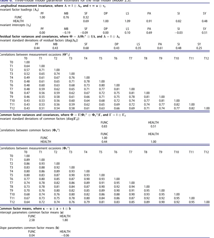
Table 6. Three-mode model parameter estimates for the final model (Model 2.5).
Longitudinal measurement invariance, whereK5IK0,ands5us0
Invariant factor loadings (K0)
PF MB SF DP LS PA SI SY
FUNC 1.00 0.76 0.32
HEALTH 0.69 1.00 1.09 0.91 0.82 0.48
Invariant intercepts (s0)
PF MB SF DP LS PA SI SY
0.00 0.19 0.09 0.00 0.10 0.69 0.03 0.51
Residual factor variances and covariances, whereH¼D(HT I)D,andD¼ID0
Invariant standard deviations of residual factors (diag(D0))
PF MB SF DP LS PA SI SY
0.44 0.43 0.68 0.43 0.35 0.61 0.48 0.25
Correlations between measurement occasions (HT)
T0 T1 T2 T3 T4 T5 T6 T7 T8 T9 T10 T11 T12
T0 1.00
T1 0.64 1.00
T2 0.57 0.71 1.00
T3 0.52 0.65 0.74 1.00
T4 0.49 0.61 0.67 0.76 1.00
T5 0.48 0.61 0.65 0.71 0.78 1.00
T6 0.48 0.60 0.63 0.68 0.73 0.80 1.00
T7 0.48 0.59 0.62 0.65 0.71 0.77 0.81 1.00
T8 0.47 0.56 0.59 0.62 0.67 0.72 0.75 0.81 1.00
T9 0.46 0.55 0.58 0.61 0.66 0.71 0.75 0.78 0.81 1.00
T10 0.43 0.53 0.56 0.60 0.64 0.68 0.72 0.74 0.77 0.81 1.00
T11 0.43 0.53 0.56 0.59 0.62 0.65 0.69 0.72 0.74 0.77 0.82 1.00
T12 0.43 0.51 0.54 0.58 0.61 0.63 0.66 0.69 0.71 0.74 0.77 0.82 1.00
Common factor variances and covariances, whereU¼C(UT UV)C, andC¼IC0
Invariant standard deviations of common factors (diag(C0))
FUNC HEALTH
0.83 0.51
Correlations between common factors (UV)
FUNC HEALTH
FUNC 1.00
HEALTH 0.44 1.00
Correlations between measurement occasions (UT)
T0 T1 T2 T3 T4 T5 T6 T7 T8 T9 T10 T11 T12
T0 1.00
T1 0.89 1.00
T2 0.86 0.93 1.00
T3 0.83 0.88 0.92 1.00
T4 0.80 0.86 0.89 0.93 1.00
T5 0.80 0.83 0.87 0.90 0.93 1.00
T6 0.77 0.80 0.85 0.87 0.90 0.93 1.00
T7 0.74 0.78 0.82 0.86 0.89 0.91 0.95 1.00
T8 0.73 0.78 0.81 0.84 0.87 0.90 0.92 0.94 1.00
T9 0.70 0.76 0.80 0.82 0.85 0.89 0.90 0.91 0.95 1.00
T10 0.68 0.74 0.76 0.80 0.82 0.86 0.88 0.90 0.93 0.95 1.00
T11 0.67 0.73 0.75 0.78 0.80 0.84 0.86 0.87 0.92 0.92 0.95 1.00
T12 0.64 0.72 0.74 0.76 0.79 0.81 0.83 0.85 0.89 0.90 0.92 0.95 1.00
Common factor means, wherej¼uaþtb Intercept parameters common factor means (a)
FUNC HEALTH
2.58 1.80
Slope parameters common factor means (b)
FUNC HEALTH
0.04 0.06
Notes: The variance-covariance structure of the final model, i.e.,R¼K U K’þH, is modeled by imposing the following Kronecker product restrictions: R¼(IK0)( (IC0) (UT UV) (IC0)) (IK0)’þ(ID0)(HT I) (ID0).
example of bone metastases, only the hypothesis of equal residual variances seems tenable. This indicates that the unique variance of each indicator stays stable across time.
Common factor variances and covariances:
Imposition of the Kronecker product restriction on the matrix of common factor variances and covarian-ces yields 94 estimates to compute 351 parameters (i.e., the total number of common factor variances and covariances), thus having a large impact on model parsimony. Moreover, in our example of bone metas-tasis, it might be interesting to investigate whether the change in the variances and covariance of the under-lying factors is proportionate over time. The model with Kronecker product restrictions imposed on both the common factor correlations and the common fac-tor standard deviations yielded close fit according to the RMSEA and CFI (Model 2.3 b, Table 5) and can be considered to show equivalent approximate fit compared to the model with free common factor var-iances (CHISQdiff (258)¼685.3, p<.001;
ECVIdiff¼0.11 95% CI:0.03 to 0.26; CFIdiff¼0.004).
Therefore, this model is retained and used as the ref-erence model in subsequent model comparisons below. This result indicates that the standard devia-tions of the common factors functional limitadevia-tions and health impairments and their correlation, change proportionately over time. The total number of free parameters in this model is 230.
Substantive hypotheses: It might be of interest to
test whether the variances of functional limitations and health impairments are invariant across time, or whether the relationship between functional limita-tions and health impairments is invariant across time. Models 2.3c, 2.3d, and 2.3e are used to test equality of common factor variances, correlations, and covarian-ces, respectively. The hypothesis of equal common factor variances across occasions should be rejected based on the chi-square difference test, but based on the ECVI difference test and the CFI difference the model with equal common factor variances can be retained (CHISQdiff (12)¼37.6, p < .001;
ECVIdiff¼0.01, 95% CI: 0.01 to 0.06;
CFIdiff<0.001). Moreover, the overall model fit of this
model is still considered to be good. The hypotheses about equal correlations and thus covariances across occasions must be rejected based on the chi-square difference and ECVI difference tests, but might be retained based on the CFI difference (CHISQdiff
(64)¼305.2, p<.001; ECVIdiff¼0.23 95% CI:
0.13–0.34; CFIdiff¼0.002). Taken together, these
results indicate that only the hypothesis of equal
common factor variances is tenable. This entails that both the individual variability in the common factors and the covariance between the two common factors are stable across time.
Common factor means: In order to investigate the
longitudinal development of the underlying factors functional limitations and health impairments, Kronecker product restrictions were imposed to test (possible) changes in common factor means across time. The model with Kronecker product restrictions on the common factor means yielded close fit accord-ing to the RMSEA, and good fit accordaccord-ing to the CFI (Model 2.4a, see Table 5). The model that imposes a linear trend on the means of the common factors (Model 2.4b) can be considered to show equivalent approximate fit (CHISQdiff (10)¼32.1, p<.001;
ECVIdiff¼0.01 95% CI: 0.01 to 0.05; CFIdiff<0.001),
whereas the model that imposes equality of common factor means across occasions (Model 2.4c) shows a significant deterioration in model fit according to the chi-square difference and ECVI difference tests, but should not be rejected based on the CFI difference (CHISQdiff (12)¼57.9, p<.001; ECVIdiff¼0.04 95%
CI: 0.01–0.09; CFIdiff<0.001). These results indicate
that there is a significant change in the common fac-tor means across time, and that this change can be described using a linear trend.
The final model: The model that includes all
Kronecker product restrictions deemed tenable based on the results reported above would be a plausible final model. The final L3MM thus includes Kronecker product restrictions on the factor loadings and inter-cepts to comply with measurement invariance (Model 2.1), on the residual variances and covariances (Model 2.2b), on the common factor variances and covarian-ces (Model 2.3b), and on the common factor means (Model 2.4a). In addition, the final model includes equality restrictions on residual factor variances (Model 2.2c) and common factor variances (Model 2.3c), and imposes a linear trend on the common fac-tor means (Model 2.4b). The resulting final model yielded close fit according to the RMSEA, and good fit according to the CFI (Model 2.5, see Table 5). This L3MM required only 184 parameter estimates, and gained 1090 degrees of freedom as compared to the measurement model (Model 1.1).
Interpretation of parameter estimates: To illustrate
the interpretation of L3MM parameters, we will exam-ine the parameter estimates of the final model (Model 2.5) that are given inTable 6.
Factor loadings and intercepts: In the final L3MM,
time, i.e., K5I K0, and s5u s0 respectively
(see Table 6). For example, the element k052 is the
estimated factor loading of the observed indicator list-lessness, that applies to all measurement occasions (i.e., k052¼1.09). The element s05 is the invariant intercept value that was estimated for the same indicator.
Residual factor variances and covariances: In the
final L3MM, the Kronecker product restrictions imposed on Himply that residual factor variances are equal across time, and that the correlations between residual factors change proportionately, i.e.,
H¼D(HT I)D, and D¼I D0 (see Table 6). Thus, the first element of D0 is the estimate of the invariant standard deviation of the residual factor of physical functioning (D011¼0.44), that is used for the computation of the residual variance of 0.20 (¼ 0.442) for all indicators of physical functioning across time. Estimates of HT* are the correlations between meas-urement occasions. The factor by which the relation-ships between the residual factors change across occasions is equal for all residual factors, but the actual covariances between the residual factors across occasions may differ because they are dependent on the standard deviations of the indicators. Also, it is now easy to see that correlations between measure-ment occasions decrease as the lag between the occa-sions becomes larger (i.e., the correlation between the first and the second measurement occasion is larger than the correlation between the first and third meas-urement occasion, and so on). In addition, correla-tions between measurement occasions of the same lag increase over time, i.e., the correlation between the first and the second measurement occasion is smaller than the correlation between the second and the third measurement occasion, and so on. This pattern of correlations explains why the restriction of equal cor-relations of the same lag (i.e., Model 2.2d) was not tenable. It might be, for example, that patients get used to the repeated assessments and therefore answer the questions in a more homogenous way.
Common factor variances and covariances: In the
final L3MM, the imposed Kronecker product restric-tions on U imply that common factor variances are equal across time, that the covariance between the common factors of the same measurement occasion is equal across time, and that the correlations between common factors of different measurement occasions change proportionately, i.e., U¼C(UT UV)C,
and C¼I C0 (see Table 6). The estimates of the
invariant standard deviations of the common factors functional limitations and health impairments (C0) are
0.83 and 0.51, respectively, and the correlation between the two common factors at the same meas-urement occasion (UV*) is 0.44. The invariant covari-ance between the two common factors of one measurement occasion is thus 0.19 (i.e., 0.44 0.83 0.51). Correlations between measurement occasions (UT*) show the change in correlations between meas-urement occasions across time, e.g., correlation between measurement occasions decrease as the lag between measurement occasions becomes larger. Although correlations between measurement occasions apply to both common factors, actual covariances between common factors across occasions differ as they are dependent on the standard deviations of the common factors. Similar to the pattern of correlations between measurement occasions of residual factors, the result of the common factors shows a decrease in correlations between measurements as the lag between the occasions becomes larger, while correlations between measurement occasions of the same lag increase over time. This indicates that patients become more homogenous in their answers to the observed variables of physical limitations and health impair-ments over time.
Common factor means: In the final L3MM, the
lon-gitudinal development of common factor means is described by a linear trend, i.e., j¼u aþt b
(see Table 6). The intercept parameters (a1 and a2)
are equal to the common factor means at the first measurement occasion. The slope parameters (b1 and b2) represent the linear change in common factor means across occasions, where the means of the com-mon factor functional limitations increase across occa-sions (b1¼0.04), while the means of the common factor health impairments decrease across occasions (b2¼ 0.06). However, only the decrease in health impairments was statistically significant based on the associated standard error of the slope parameter. The complete vector of common factor means is computed as a function of time of measurement. These results may indicate possible effects of patients’ coping strat-egies, as the relatively objective indicators of func-tional limitations remain stable (e.g., physical functioning, mobility), whereas the more subjective indicators of health impairments (e.g., depression, pain) decrease over time.
Discussion
very parsimonious models, enabling the application of SEM to large longitudinal data sets. In the present paper we explained and illustrated the imposition of Kronecker product restrictions on the parameter matrices of (1) factor loadings and intercepts to com-ply with the assumption of longitudinal measurement invariance; (2) residual factor covariances and correla-tions, and additional restrictions to test equality of variances, correlations and covariances across occa-sions; (3) common factor covariances and correlations, and additional restrictions to test equality of variances, correlations, and covariances across occasions; and (4) common factor means, and additional restrictions to test a linear trend of common factor means. In add-ition, we explained how the resulting parameter esti-mates can be interpreted. This paper, therefore, serves as an instructive description of L3MMs in order to facilitate their applications for complex longitudinal data and to enhance the substantive interpretation of model parameters. However, the illustration in the current tutorial also showed that model fit evaluation is not straightforward for these types of parsimonious models. Therefore, in the following, we address the challenges with regard to evaluation of (differences) in model fit in more detail, suggest areas for future research, and provide recommendations for research-ers and practitionresearch-ers who wish to apply the L3MM in an informative way.
The main benefit of the L3MM is that it enables the modeling of multivariate longitudinal data from many measurement occasions within the general and versatile SEM framework. When applying L3MMs one can thus profit from general SEM features and devel-opments, such as methods for handling missing data (e.g., using alternative estimators), and diagnostics of possible misfit in (parts of) the model (e.g., using cor-relation residuals or modification indices) (cf. Bollen,
1989; Kline, 2011). The L3MM is especially suited for analyses of data from many measurement occasions (i.e.,>2) with fixed intervals between occasions. However, the L3MM can become of unmanageable size with very large numbers of occasions (e.g., with 50 occasions, the decomposition will yield a matrix of dimensions 5050) and alternative modeling strat-egies are more appropriate (cf. Hamaker, Ceulemans, Grasman, & Tuerlinckx, 2015). Moreover, some gen-eral SEM guidelines may not be applicable to the spe-cific L3MM context, such as sample size requirements or model fit evaluation, the latter of which we elabor-ate on below.
L3MMs are applied to assess change in multivariate longitudinal data with many measurement occasions.
The size of these types of models is usually large in terms of observed variables and model parameters. For example, in our sample of 682 patients with bone metastases we modeled 104 observed variables meas-ured over 13 measurement occasions, which resulted in a measurement model that required estimation of 1274 model parameters with 4290 degrees of freedom. Evaluation of model fit is complicated by the fact that the chi-square test of exact fit is dependent on sample size and number of degrees of freedom (i.e., with increasing sample size and equal degrees of freedom the chi-square value increases) and tends to favor highly parameterized models (i.e., the chi-square value decreases when parameters are added to the model). The RMSEA and CFI indices of approximate fit are less dependent on sample size and reward model par-simony. In our illustration with the L3MMs the evalu-ations of overall model fit indicated that none of the models showed exact fit according to the chi-square test, while all models showed close approximate fit (RMSEA <0.05). The CFI index seemed to be some-what more discriminative as not all models showed good fit (CFI >0.95), but without confidence intervals for these values the precision of the index is unknown. Therefore, this raises the question of how informative these overall model fit measures are in the case of highly parsimonious (longitudinal) models. Existing guidelines are based on simulation studies that have addressed the performance of overall good-ness of fit measures, with relatively simple, single-occasion examples (cf. Hu & Bentler, 1999). It may be the case that highly parsimonious models with large numbers of degrees of freedom require alternative fit indices or decision rules for an accurate evaluation of overall goodness of fit. For example, the RMSEA may not have enough discriminative power when models are very parsimonious (i.e., have many degrees of freedom). The CFI may not be informative with longi-tudinal data analyses, as the null model (i.e., a model without correlations between variables) is too unrealis-tic in the case of repeated measures of the same varia-bles across time. As complex longitudinal models will only become more prevalent in the presence of large data sets, it would be worthwhile to investigate the behavior of overall model fit indices as a topic of future research.
freedom, evaluation of difference in model fit is com-plicated for the same reasons as described above. As an alternative to the chi-square difference test, we used the difference in ECVI and CFI values to evalu-ate differences in model fit. An advantage of the ECVI difference is that the associated confidence interval provides information about the precision of the estimate and allows to test the equivalence in approximate model fit. In our application, the chi-square difference test showed the highest power, rejecting all the L3MM restrictions (i.e., Kronecker product restrictions on parameter matrices), and all but one of the additional restrictions on L3MM par-ameter matrices to test substantive hypotheses. The ECVI difference test showed that some of the L3MM restrictions and substantive hypotheses could be retained based on the evaluation of equivalence in approximate fit, whereas the CFI difference showed the least discriminative power as almost all models could be retained based on the rule of thumb for this index (CFIdiff¼0.01). Thus, our illustration seems to
indicate that the ECVI difference may be more informative for the evaluation of differences in model fit than the differences in chi-square or CFI values. However, stringent evaluation of the performance of the ECVI for the comparison of nested models has not yet been performed. Future research is needed to address the appropriateness of the ECVI difference in various contexts. Although the Kronecker product restrictions represent the data well and aid interpret-ation, it is difficult to provide decision rules for when the assumption of proportional change does not hold. Simulation studies are required to provide guidelines on how to address model fit evaluation in these circumstances.
Due to the problems in evaluating overall model fit and differences in model fit there is a risk of retaining an incorrect solution. Although Kronecker product restrictions lead to simpler – and thus more favorable
– models according to the parsimony principle, one should be aware that very restrictive models may lead to biased parameter estimates. A rigid adherence to the parsimony principle could thus lead to bias and misinterpretation in model evaluation and selection. Unfortunately there is a lack of studies about when and to what extent parameters may be biased when the Kronecker product restrictions do not hold, thus complicating decisions on model fit evaluation. Therefore, we want to emphasize that statistics alone are not sufficient to guide decisions regarding these types of model evaluations, and that such decisions require substantive guidance as well. For example, the
evaluation of difference in model fit can be used to test the tradeoff between model fit and model parsi-mony, but may also be affected by interpretability of results. In our illustration we incorporated Kronecker product restrictions on residual factor variances and covariances, even though these restrictions yielded deterioration in model fit. In part, we chose to incorp-orate these restrictions in favor of model parsimony and interpretability of results. Instead of yielding 104 estimates of residual factor variances and 624 esti-mates of residual factor covariances, the L3MM yielded eight estimates of residual factor variances, and 90 estimates that represent the proportional change in residual factor variances and covariances over time. These restrictions thus facilitate the sub-stantive interpretation of model parameters –not only in terms of their number but also in terms of their meaningfulness due to the specifics of the L3MM decomposition. The argument to favor parsimonious models only when they facilitate interpretation has been made previously by others as well (e.g., Mulaik,
As a recommendation for researchers and practi-tioners that apply these types of models, we would suggest to (1) use several tests and indices of model fit in order to find support for the robustness of the result in their commonalities, (2) keep in mind that some fit indices are more appropriate in certain cir-cumstances than others (e.g., specifically developed to take into account model parsimony), and (3) take into account substantive considerations when making deci-sions on model fit evaluation (e.g., using theory to establish an appropriate measurement model in add-ition to relying on model fit tests or indices to guide the specification of a measurement model) (see also Verdam,2017).
To conclude, this paper provides an instructive application of the L3MM for multivariate longitudinal data from many measurement occasions. Kronecker product restrictions are used to model the multivariate longitudinal structure of the data, which yields models that are more parsimonious and have attractive inter-pretation. Application of the L3MM therefore facili-tates the analysis of complex longitudinal data and can provide meaningful interpretation of the dynamics of change. However, future research is needed in order to support statistical decision rules for the ten-ability of Kronecker product restrictions and other substantive hypotheses in general. Such research will facilitate future applications of the L3MM and thus further our understanding of longitudinal dynamics within the life sciences.
Article information
Conflict of interest disclosures:Each author signed a form for disclosure of potential conflicts of interest. No authors reported any financial or other conflicts of interest in rela-tion to the work described.
Ethical principles:The authors affirm having followed pro-fessional ethical guidelines in preparing this work. These guidelines include obtaining informed consent from human participants, maintaining ethical treatment and respect for the rights of human or animal participants, and ensuring the privacy of participants and their data, such as ensuring that individual participants cannot be identified in reported results or from publicly available original or archival data.
Funding: This work was supported by KWF-Grant 2011-4985 from the Dutch Cancer Society.
Role of the funders/sponsors: None of the funders or sponsors of this research had any role in the design and conduct of the study; collection, management, analysis, and interpretation of data; preparation, review, or approval of the manuscript; or decision to submit the manuscript for publication.
Acknowledgements: The authors would like thank Y. M. van der Linden for making the data from the Dutch Bone Metastasis Study available for secondary analysis. Both authors participate in the Research Priority Area Yield of the University of Amsterdam. The ideas and opinions expressed herein are those of the authors alone, and endorsement by the authors’ institutions or the funding agency is not intended and should not be inferred.
References
Akaike, H. (1987). Factor analysis and AIC. Psychometrika,
52(3), 317–332. doi:10.1007/BF02294359
Bentler, P. M. (1990). Comparative fit indexes in structural models. Psychological Bulletin, 107(2), 238–246. doi:
10.1037/0033-2909.107.2.238
Bentler, P. M., & Chou, C.-P. (1987). Practical issues in structural modeling.Sociological Methods Research, 16(1), 78–117. doi:10.1177/0049124187016001004
Bentler, P. M., Poon, W.-Y., & Lee, S.-Y. (1988). Generalized multimode latent variable models: Implementation by standard programs. Computational
Statistics & Data Analysis, 7(2), 107–118. doi:10.1016/
0167-9473(88)90086-2
Bentler, P. M., & Lee, S.-Y. (1979). A statistical development of three-mode factor analysis. British Journal of
Mathematical and Statistical Psychology, 32(1), 87–104.
doi:10.1111/j.2044-8317.1979.tb00754.x
Bloxom, B. (1968). A note on invariance in three-mode fac-tor analysis. Psychometrika, 33(3), 347–350. doi:10.1002/ j.2333-8504.1967.tb00554.x
Boker, S., Neale, M., Maes, H., Wilde, M., Spiegel, M., Brick, T., … Fox, J. (2011). Openmx: An open source extended structural equation modeling framework.
Psychometrika, 76(2), 306–317. doi:
10.1007/s11336-010-9200-6
Bollen, K. A. (1989). Structural equations with latent
varia-bles. New York: Wiley. doi:10.1002/9781118619179
Browne, M. W., & Cudeck, R. (1989). Single sample cross-validation indices for covariance structures. Multivariate
Behavioral Research, 24(4), 445–455. doi:10.1207/
s15327906mbr2404_4
Browne, M. W., & Cudeck, R. (1992). Alternative ways of assessing model fit.Sociological Methods Research, 21(2), 230–258. doi:10.1177/0049124192021002005
Carroll, J. D., & Chang, J. J. (1970). Analysis of individual differences in multidimensional scaling via an n-way gen-eralization of Eckart–Young decomposition.
Psychometrika,35(3), 283–319. doi:10.1007/BF02310791
Cheung, G. W., & Rensvold, R. B. (2002). Evaluating good-ness-of-fit indexes for testing measurement invariance.
Structural Equation Modeling, 9(2), 233–255. doi:10.1207/
S15328007SEM0902_5
Crowder, M. J., & Hand, D. J. (1990). Analysis of repeated measures. New York: Routledge.
Dudgeon, P. (2003). NIESEM: A computer program for cal-culating noncentral interval estimates (and power analysis) for structural equation modeling. Melbourne: University of Melbourne, Department of Psychology.