www.ijemst.com
Exploring Foundation Concepts in
Introductory Statistics Using Dynamic
Data Points
George Ekol
Simon Fraser University
To cite this article:
Ekol, G. (2015). Exploring foundation concepts in introductory statistics using dynamic data
points.
International Journal of Education in Mathematics, Science and Technology, 3
(3),
230-241.
This article may be used for research, teaching, and private study purposes.
Any substantial or systematic reproduction, redistribution, reselling, loan, sub-licensing,
systematic supply, or distribution in any form to anyone is expressly forbidden.
Authors alone are responsible for the contents of their articles. The journal owns the
copyright of the articles.
Volume 3, Number 3, July 2015, Page 230-241
ISSN: 2147-611X
Exploring Foundation Concepts in Introductory Statistics using Dynamic
Data Points
George Ekol*
Simon Fraser University
Abstract
This paper analyses introductory statistics students’ verbal and gestural expressions as they interacted with a dynamic sketch (DS) designed using Sketchpad software. The DS involved numeric data points built on the number line whose values changed as the points were dragged along the number line. The study is framed on aggregate reasoning with quantitative data, but it also draws on the Vygotskian social cultural and historical perspective of learning, particularly, how cultural artefacts including language support learning. Three concepts, namely, data distribution, the mean and standard deviation were analyzed in the study. Tasks were designed such that students first talked about their informal understanding of the three concepts before interacting with the DS; then they interacted with the DS and discussed the connections among the three concepts as they dragged the data points along the horizontal axis. Analysis of students’ verbal, gestural and other expressions suggest firstly, that the dynamic sketch mediated the informal meaning of data variability for them, particularly the meaning of standard deviation, which most students only recalled through a formula. Secondly, the interactions with the DS drew students’ attention away from focusing on formulas and calculations which was clearly evident in their statements before the DS was introduced, to investigating the connections among concepts. These findings support previous studies that have proposed that the use of dynamic computing tools strongly support students’ informal understanding of abstract concepts. Implications for teaching and learning introductory statistics concepts at the tertiary level are discussed.
Key words: Introductory statistics, Variability, Sketchpad, Dynamic sketch, Standard deviation, Aggregate
reasoning.
Introduction
Statistical thinking, reasoning and literacy (STRL) are important learning goals in statistics education and have attracted the attention of many researchers in the recent past (e.g., see Garfield & Ben-Zvi, 2008). Reasoning with quantitative data is particularly important given that the volume of quantitative data that inundate our social and economic world is huge and is growing every day. This mass data often demand careful analysis toward decision making both at individual, but also at group level. It is thus important that students should learn data handling skills at school as they prepare for the world of work. However, to successfully derive meaning from quantitative data, the notions of variability and aggregate reasoning need to be understood (Konold, Higgins, Russell, and Khalil, 2014). According to Konold, Higgins, Russell, and Khalil (2014), students are more likely to view numerical data in four categories, namely, data as: i) pointers, ii) case-values, iii) classifiers and iv) aggregate. Considering data as pointers involves focusing on issues outside the data set itself, such as discussing the data collection process rather than the distribution of data whereas viewing data as case-values involves focusing on particular data points such as the largest value, or the smallest value in a data set. Classifier reasoning with data, Konold et al. propose, is about counting individual data values having the same attributes. For example, counting how many times data points with a specific numeric value or above that value appear in the entire data set. Lastly, according to Konold and colleagues, aggregate reasoning includes paying attention to the overall distribution of the entire dataset, including identifying the center of data and the overall deviation of data values from the center. In general, aggregate reasoning with data is more demanding cognitively to students than the other levels of reasoning with data (e.g., Hardiman, Well, & Pollatsek, 1984; Konold et al. 2014; Konold & Higgins, 2003; Bakker & Gravemeijer, 2004; Hancock et al.,1992; Konold et al., 1997; Mokros &
*
Russell, 1995; delMas & Liu, 2005; Garfield & Ben-Zvi, 2008). In fact, research suggest an association between aggregate reasoning with data and understanding of the foundation concepts such as variability (Wild & Pfankuch, 1999), distribution and standard deviation (delMas & Liu, 2005) and the mean (Hardiman, Well, & Pollatsek, 1984; Stigler, 1999). The purpose of the this study therefore, is to explore how a dynamic sketch implemented in a computer environment can support students’ informal reasoning about the three foundation concepts mentioned above and develop their aggregate reasoning with data. The next section briefly discusses the theoretical perspectives that were adapted in the study.
Theoretical Perspectives
Given that the current study involves reasoning with data, the theories of statistical thinking and aggregate reasoning are employed (e.g., Konold, Higgins, Russell, and Khalil, 2014; Wild & Pfannkuch, 1999). The study also draws on the Vygotskian social cultural and historical perspective of learning, which provides that specific cultural tools including language can promote learning in a given cultural community, in this sense, a mathematical community. With regard to specific cultural tools, Sketchpad (Jackiw, 1991) software is used in designing tasks that support students’ informal reasoning with data, toward aggregate reasoning.
Aggregate Reasoning with Data
Several researchers agree that when learners view data in aggregate, their focus shift from individual cases to the integrating the overall shape of the distribution (Wild & Pfannkuch, 1999; Watson, 2005; Pfannkuch & Wild, 2004; Konold & Pollatsek, 2002; Hancock, Kaput, & Goldsmith, 1992; Konold et al. 2014; Konold & Higgins, 2003). The aggregate perspective is summarized by Pfannkuch and Wild (2004) who state that:
Individual–based reasoning concentrates on the single data points and with little attempts to relate them to the wider data set, whereas aggregate-based reasoning is concerned with patterns and relationships in the data set as a whole. (p. 20)
Hancock, Kaput, and Goldsmith (1992) propose that students’ ability to reason from group tendencies rather than from individual cases is fundamental to developing their statistical thinking. Other researchers (e.g., delMas & Liu, 2005), building on the same foundation of aggregate reasoning have used dynamic graphs to enable students visualize patterns in the data distributions and reason about the variations in the data sets. However, the problems related to data variability and aggregate reasoning are not yet exhausted. The current study investigates another angle whereby students physically drag data points on the computer screen and discuss the changes in the data distribution in real time. The study is framed on the Vygotskian theory of learning whereby cultural tools and language can be used to promote learning and understanding in a community. Moreover tools can also be used to provide specific signs that can mediate meanings and promote understanding in a given community (Falcade, Laborde, Mariotti, 2007; Bartolini Bussi, & Mariotti, 2008; Arzarello, Paola, Robutti, & Sabena, 2009; Vygotsky, 1978). In this study, a cultural community is the defined as a mathematical community, including a mathematics classroom.
How Tools Function As Signs for Learning Mathematical Concepts
Research studies have shown that physical (corporeal) tools can be used to support students learn the meanings of mathematıcal concepts (Falcade, Laborde, Mariotti, 2007; Bartolini Bussi, & Mariotti, 2008; Arzarello, Paola, Robutti, & Sabena, 2009; Vygotsky, 1978). According to the Vygotskian theory of learning, a cultural tool can be used to promote leaning of concepts through the signs that it generates (e.g. Vygotsky, 1978; Falcade, Laborde & Mariotti, 2007; Bartolini Bussi & Mariotti, 2008). Take for example two square shapes, A and B, with square A larger than square B. One could through visualization, state that ‘the area of square A is bigger than area B’, which, according to the Vygotskain perspective is categorized as a mathematical statement and is cognitive. In the Vygotskian sense then, a physical drawing serves an external function whereas a sign serves a cognitive function (Bartolini Bussi & Mariotti, 2008). The apparent transformation from a physical tool into an cognitive function tool is termed internalization (Wertsch & Addison Stone, 1985).
reasoning with data in aggregate by visualizing the relationships in the data distributions. The study aims to answer the following specific research questions are:1) How do introductory statistics students reason about the notions of distribution, the mean and standard deviation without the dynamic sketch; 2) How are students’ reasoning about the notions of distribution, the mean and standard deviation different after interacting with the dynamic sketch?; and 3) In what ways does the dynamic tool contribute to students’ aggregate reasoning with numerical data? Drawing on the theoretical perspectives discussed above and also on other research studies, I hypothesize that students’ thinking about the three foundation concepts before interacting with the dynamic sketch will show more deterministic reasoning focused on formulas calculations. But after interacting with the dynamic sketch, students reasoning will informally show some aggregate reasoning with quantitative data.
Method
Participants
The study participants were five undergraduate students from a large research and teaching university in NorthWestern Canada. The participants, except for one student who had completed introductory statistics in the previous semester, were at the time of the interview enrolled in a 14-week introductory statistics course conducted by instructors at the Department of Statistics and Actuarial Science. The five students in my study were familiar with statistical data analysis software such as JMP and SPSS, but they had not used Sketchpad software before. However, before the interviews, participants were given ample time to practice with Sketchpad software and none of the students showed any difficulty using Sketchpad during the interviews. Participants’ general familiarity with other computer software may have eased their quick adaptation to Sketchpad software functions during the interviews.
Materials
By the time of the interview participants had learned in their statistics classes and also from the course text books (e.g. Moore, 2010) the concept of distribution (e.g., describing distributions with graphs such as bar graphs, pie charts, box plots, histograms and stem plots). They had also learned describing distributions with numbers (e.g., the mean, mode, median, and standard deviation) as well as learned the about the normal distribution curve (e.g., the normal density curve, the 68-95-99.7 rule and applying the rule for obtaining a probability under the standard normal). The study participants were obviously familiar with the formula for obtaining the mean
n i
i
x
in
1
)
/
1
(
of a data set,x
iis the individual data point and n is the number of data points in the data set. The participants had also learned about standard deviation and its relationship with the mean and data distribution. Previous research studies (e.g. delMas & Liu, 2005) however, revealed that students generally struggle with the meaning of standard deviation even if they do not show much difficulty using theformula 2 (1/2)
1
(
)
]
))
1
/(
1
[(
n
i nx
x
i i
for calculating the value of standard deviation from a numerical dataset. Therefore the interview tasks were designed on the Sketchpad to enable students visualize changes in standard deviation in relation to changes in the mean and data distribution as they physically dragged the data points on the number line. Sketchpad software was chosen among other dynamic software for two reasons. First, the software was found to be highly adaptable and easy to use. Secondly, Sketchpad functions directly involved the students in the learning process in real time in the sense that participants were able to drag data points in the computer environment and watch the changes. In that respect, Sketchpad directly supported students’ exploration and discovery (Arzarello et al. 2002) through dragging data points on the dynamic sketch and students noticing what changed and what did not change on the sketch.Data Collection Instrument
Analysis of the Instrument
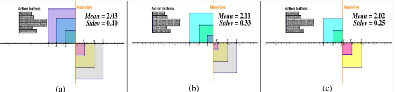
Figure 1 is the dynamic sketch (DS) used for collecting data. The term ‘dynamic’ is applied in the sense that a numeric data point constantly changes its numerical value as it is dragged along the number line. The term “data point” is applied in this study to mean both the location of the data (e.g., at position marked A) on the horizontal axis in the DS and its numeric value. Dragging action involves selecting a data point, or a group of data points on the DS, holding down the left side of the mouse and gently dragging the mouse on the number line. I refer to the system of tools used for dragging data points on the DS as the dragging tool. To drag all the data points together, all the points are selected, but only one of the selected points is dragged in the desired direction. That action enables all the selected points to move the same distance in the same direction. Figure 1(a) is a simplified version of the DS having six dynamic data points A, B, C, D, E and F on the number line. As a data point is dragged on the number line, the numeric values of the mean and standard deviation increase or decrease according to whether the data point is dragged toward the center of the dataset or away from the center of the dataset. Sketchpad software makes it possible to add as many data points as possible, but in this investigation a small dataset was chosen to minimize overcrowding the sketch and distracting students' attention from focusing the relationships among standard deviation, the mean and data distributions on the number line as they dragged the data points on the horizontal number. The DS is also designed with numeric scales that enable student read off the values of the mean and standard deviation during the dragging action. The action buttons on the DS enable the dynamic specific functions of Sketchpad to be hidden from students during prediction stages and the buttons are activated when students have to check the in predictions. To activate a button, one simply clicks on Show<function>, e.g. Show <mean> to show the mean. Clicking once on the 'Show mean' button one activates the numeric values of the mean; clicking it again hides the numeric values of mean.
0.6 0.8 1 1.2 1.4 1.6 1.8 2 2.2 2.4 2.6 2.8
Stdev = 0.40
Mean = 2.03
Action buttons Mean-line
Hide Measurement Stdev Show Curve Hide Measurement Mean Hide squares Hide Mean
Hide Unit Points
m B C D E A F (a)
0.6 0.8 1 1.2 1.4 1.6 1.8 2 2.2 2.4 2.6 2.8
Stdev = 0.33
Mean = 2.11
Action buttons Mean-line
Hide Measurement Stdev Show Curve Hide Measurement Mean Hide squares Hide Mean
Hide Unit Points
m B C D E A F (b)
0.6 0.8 1 1.2 1.4 1.6 1.8 2 2.2 2.4 2.6 2.8
Stdev = 0.25
Mean = 2.02
Action buttons Mean-line
Hide Measurement Stdev Show Curve Hide Measurement Mean Hide squares Hide Mean
Hide Unit Points
m B C D E A F (c)
Figure 1. (a) Before dragging the data points; (b) Data point A on the extreme left is dragged to the right toward the mean line, the mean value increases as standard deviation decreases; (c) Data point F originally placed on the right side of the mean-line is dragged to the left; both the mean and deviation standard decrease relative to
Figure 1(a).
Sketchpad simulates the numeric values for the mean and standard deviation from their algebraic expressions
n i
i
x
in
1
)
/
1
(
and 2 (1/2)1
(
)
]
))
1
/(
1
[(
n
i nx
x
i i
respectively. For instance, in Figure 1(a), the mean of thesix data points marked A, B, C, D, E, and F on the number line is given by
(
1
/
)
62
.
03
1
i
i
x
in
and thecorresponding standard deviation is 6 2 (1/2)
1
(
)
]
))
1
/(
1
[(
n
iix
i
x
=0.40. A perpendicular line that we
named the ‘mean-line’ is constructed at the mean point of the six data points. The mean-line (Ekol, 2013) serves two major roles: i) it provides is a physical representation of the mean of the data points during the dragging action; ii) the mean-line also serves as a tracking device for the direction where the center of the data distribution is moving with dragging. For coding purposes, (see later) it is proposed that data points that are on the left-side of the mean-line do not cross to the right- side and that those on the right-side do not cross the mean-line to the left-side. But this is only a simplification for coding purposes as will soon be shown in the next paragraph. In general, however, any data can be dragged across mean-line. In that regard, therefore, the second proposition is that if a data point or a set of data points are dragged across the mean-line, they automatically assume the coding protocol for that side of the mean-line. Data points on the left-side of the mean-line are coded with subscript“L” for “left”, e.g., AL, BL, and CL; and data points on the “right” side of the mean-line are
coded withsubscript “R” for “right”, e.g., DR, ER, and FR respectively (Fig.1a). If AL is dragged to its left, it is
coded ALL, and if dragged to its right, the coding is ALR. Similarly, for data points on the right side, for example,
if DR, is dragged to its left, it is coded DRLand if it is dragged to its right, the coding is DRR. Table 1 provides
increase in mean and standard deviation when a data point is dragged to the left or to the right of the mean-line. For example, in Figure 1a, data point AL (mean=2.03, standard dev.=0.40) on the left of the mean line shows an
increase (⇧) in the mean value from 2.03 to 2.11 and a decrease (⇩) in standard deviation from 0.40 to 0.33, when point A is dragged to its right, ALR ( see Fig. 1b). In general, the mean increases if a data points on the left
side of the mean line is dragged to the right while standard deviation decreases. Conversely, the mean decreases as standard deviation increases if a data point on the left of the mean-line is dragged to the left. However, on the right side of the mean-line, both the mean and standard deviation increase in magnitude if data points are dragged to the right; and they both decrease if data points are dragged to the left. For each data, two possible directions of movement are coded to the left or right, but in Table 1, only a few codes are shown as examples. The uncompleted parts are represented by “–”, but it is not difficult to complete the changes for each data point. Altogether there are 14 possible directions of dragging, two for each of the six individual data points, and two for all the data points dragged together to the left or to the right. The last two rows in Table 1 provides that if the six data points are selected and all dragged together the same distance to the left, or to the right, standard deviation stays constant, but the mean decreases (⇩) as the points are dragged to the left and increases (⇧) as the points are dragged to the right. This finding shown graphically on the DS through dragging action is an important statistical principle that often eludes many introductory statistics students as the students only focus on calculations. Part of the problem could be that students lack suitable tools such as the DS with which to explore dynamically and visually the association that exists between data distribution and data variability.
Table 1. The DragTable showing changes (increase or decrease) in the magnitudes of the mean and standard with the direction of dragging data points on the horizontal axis.
Direction of dragging Mean Standard
deviation ALL ALR BLL - - - FRL FRR (ABCDEF)L (ABCDEF)R ⇩ ⇧ ⇩ - - - ⇩ ⇧ ⇩ ⇧ ⇧ ⇩ ⇧ - - - ⇩ ⇧ Constant Constant
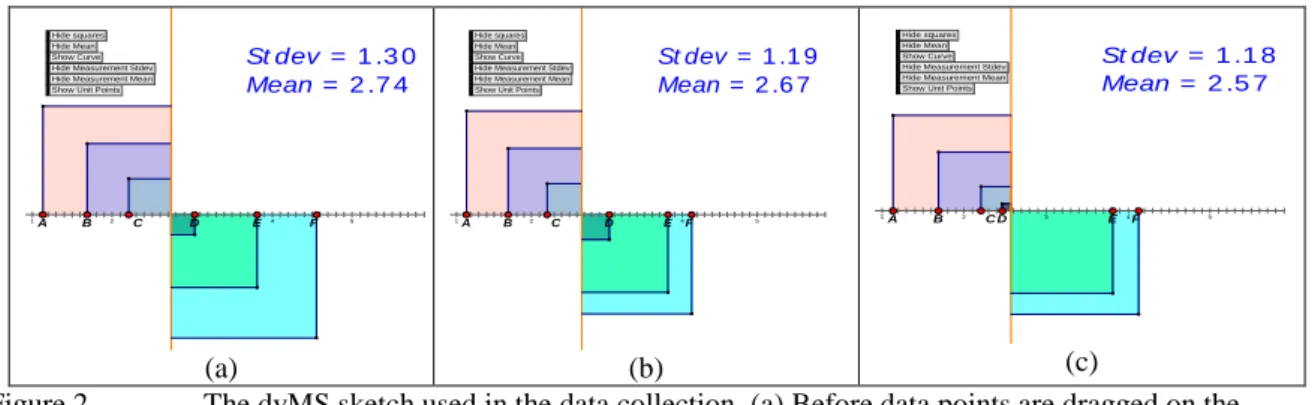
Figure 2 below extends Figure 1. Each data point is associated with a geometrical square whose length is measured from the line to the corresponding data point. For example data point A has area from the mean-line shaded pink. Although the squares overlap, each square is identified separately by its distance from the mean- line to the data point. In Figure 2(a), for instance, the magnitude of standard deviation=1.30. After data point FR (on the far right of the mean-line) is dragged slightly to its left (Fig.2(b)), the magnitude of standard
deviation decreases to 1.19; also the area of square F decreases, showing that, the farther away a data point is from the mean-line, the larger is the resultant variability in the overall dataset as reflected in the magnitude of the standard deviation. In principle, the sums of all the six squares representing the six data points provides the resultant variability of the dataset represented by the magnitude of standard deviation.
1 2 3 4 5
St dev = 1 .3 0
Mean = 2 .7 4
Show Unit Points Hide Measurement Mean Hide Measurement Stdev Show Curve Hide Mean Hide squares
F
D E
A B C
(a)
1 2 3 4 5
St dev = 1 .1 9
Mean = 2 .6 7
Show Unit Points Hide Measurement Mean Hide Measurement Stdev Show Curve Hide Mean Hide squares
F
D E
A B C
(b)
1 2 3 4 5
St dev = 1 .1 8
Mean = 2 .5 7
Show Unit Points Hide Measurement Mean Hide Measurement Stdev Show Curve Hide Mean Hide squares
F
D E
A B C
(c)
In fact, the squares were included in the design to mediate the abstract meaning of standard deviation and variability for many students. The larger the size of the square, the bigger the variability in the data set and also the larger the magnitude of standard deviation, and vice versa. As delMas, Garfield and Oom (2005) point propose, incorporating the ideas of area in graphs can help students develop understanding of theoretical distributions, and the attendant relationships.
Interview Tasks
During the interviews participants were asked to: (a) briefly state what they thought about the terms distribution, the mean and standard deviation. This task was given before participants engaged with the dynamic sketch to provide a basis for comparing any changes in their reasoning after interacting with the dynamic sketch; (b) predict and justify how the mean and standard deviation would change if data points were dragged along the horizontal number line; (c) check their predictions using Fig. 2 and talk about the changes they noticed in the data distribution, the mean and standard deviation during checking predictions; and (d) at the end, with computer closed and DS not seen anymore, reflect on the meaning of standard deviation and variability in general. The reflection in (d) was often prompted by the interviewer with a question, “What do think about the term standard deviation?” The expectation from the reflection question was two. Firstly, that after their engagement with the dynamic sketches, participants would not present the formula for standard deviation as an answer to this question, but rather, discuss or at least describe, informally what standard deviation is to the distribution of a data set. Secondly, the reflection question also served to gauge the changes in reasoning about data after their interacting with the dynamic sketch.
Data Collection
As explained in the study design, data was collection followed one-on-one, task-based interviews. Each interview session lasted between one 40-45 minutes. The interviews tasks involved semi-structured questions. In the first 10 minutes of the interview participants first answered questions that did not involve the DS. After, participants were introduced to the DS as explained earlier. The interview proceedings comprised of participants’ statements, hand movements, and gestures were videotaped and transcribed for analysis. The author watched the videotapes several times and also took screen shots of participants’ speeches and actions, e.g., hand movements and gestures during the interviews, which expressions were taken to represent their modes of reasoning about how the dataset varied along the horizontal axis. In the next section, results are presented and discussed. The square brackets [#] refer to participants' direct statements cited in the analysis. Texts enclosed in the square brackets [...] are the author’s attempts to clarify participants’ statements, but without altering the original meanings.
Results and Discussions
A large amount of qualitative data was collected in the interviews. Given that participants had all taken introductory statistics courses taught by the same instructors, it was not unexpected that their answers in the interviews would show some similarity. Data analysis was uniformly carried out for all the five participants: Anita, Boris, Halen, Maya, and Yuro. However, because of page limitation and for reasons given in the next section, only Maya’s is analyzed in more detail and supplemented by brief discussions from the other participants’ data, under section “Scanning the entire data.”
Presenting Maya’ Data
Maya’s data was chosen for detailed analysis for two main reasons. First, her data reflected the general responses seen in the other four participants’’ data. Second, Maya’s data also presented some unique features, particularly during her interactions with the dynamic sketch that other participants’ data did not present.
Maya Prior to Interacting with the Dynamic Sketch
[1] Maya: The mean is the answer to a formula where we add up all the [data] values in a particular data set and divide by the number of values that are there, so mean is like a number, like a specific number, [the] mean is more specific, it’s like calculated out.
Maya moved her hands a lot as she talked about the mean. For instance, she drew a horizontal line in the air with her right index finger as she said “and divide by the number of values that are there” [1]. Asked about standard deviation? Maya began by asking an open question, “Standard deviation?”
[2] Maya: I see standard deviation in graphs, there is like one, two, three, four; then there’s negative one, negative two, negative three, negative four. You can calculate standard deviation.
As Maya counted from one to four, she moved her right hand up and down four times; then she changed to her left hand and moved it up and down again four times as she counted from negative one to negative four. It is clear from Maya’s statements [1 & 2] that her thinking about the concept of mean relied on a “formula” for the mean, and probably also on the procedure that generates a “specific number” for the mean. For standard deviation, Maya seems to imagine a graph or “graphs” with equal distances on either side the center. The interviewer conjectured that Maya was probably referring to the normal curve with four units of standard deviations on either side of the center. The interviewer introduced Maya to the dynamic sketch in Figure 2(a), but hid the numerical values for the mean and standard deviation hidden. Maya was asked to predict how the mean and standard deviation would vary if she dragged a data point along the horizontal number line. She intently looked at the sketch for a few moments then predicted:
[3] Maya: I think when I move the points, the lines that the points are connected to will also move.
By statement [3], it was not clear what Maya meant, but the interviewer assumed that Maya meant if she dragged a data point along the horizontal line, the vertical sides of the squares would also move. The interviewer asked a more specific question about the changes in the squares, “How would the squares change as you move the data points on the horizontal number line, either to the left or to the right of the mean-line?” to which she replied,
[4] Maya: Well, I guess when I move the points to the left, the square will increase.
“Why?” the interviewer followed. Maya did not immediately respond to the last question, but stretched her right index finger toward the computer mouse pad ready to drag a data point on the dynamic sketch and check her prediction, but the interviewer intervened, “Just say what comes to your mind and then you can check after.” Maya looked at the sketch and used her right index finger to point at individual data points one after another (Fig. 3); then she responded to the last question,
[5] Maya: Because the farther away the point is from the center, then the greater area it [the square] has.
(a) (b)
Figure 3. (a) Maya points at the data points on the horizontal number line; (b) A large square shows after Maya dragged data point B to the left side of the mean-line.
slowly moved data point B (Fig. 3b) away on the left of the mean-line. She continued dragging the point back and forth and observing the changes in numerical scales of the mean and standard deviation and she said,
[6] Maya: So, the mean increases as standard deviation [pauses for a moment then continues dragging point B back and forth]. As standard deviation increases, the mean also increases. Oh no, the mean decreases right [stops dragging]. Oh, this is nice!
Maya’s statement in [6],“So, the mean increases...” suggests that she found something that was not obvious to her before interacting with the dynamic sketch. Initially, Maya assumed that an increase in standard deviation automatically meant an increase in the mean, after exploring by dragging the point, she correctly stated the changes in the mean and standard deviation. Maya’s discovery in [6] was evidently aided by the dragging action and the dragging tool of Sketchpad as she moved data point B back and forth and linked the changes in the magnitude of standard deviation with changes in the mean. Following that episode, the interviewer asked Maya what standard deviation meant to which Maya responded,
[7] Maya: Standard deviation is like a measure of how far apart the points are from the mean. Statement [7] was consistent with statement [6], but quite different from Maya’s statement [2] before she interacted with the dynamic sketch. The change in Maya’s reasoning can thus be largely associated to her interactions with the dynamic sketch by dragging points. Toward the end of the interview session, with the computer closed Maya was again asked a similar question “What do you think about standard deviation?” The question aimed at provoking Maya to reflect on the link between changes in standard deviation and changes in data distribution, but without the mediation of the dynamic sketch. Maya paused for some moments and she said,
[8] Maya: Standard deviation is certain point away from the center of a population [she stopped momentarily then continued...]. There is a formula, I forgot but, it’s like standard deviation equals the square root of the variance.
Maya’s statement [8] on the one hand, involved informally, some elements of aggregate reasoning in that she thought about the distribution of data in respect of population and center. On the other hand, Maya also reasoned about standard deviation as “equals the square root of the variance” suggesting a standard deviation was merely a pointer to a formula and to calculations. In the former case, Maya seemed to move toward an understanding of the meaning of standard deviation in an aggregate way, but in the latter, Maya took recourse to the “formula” for standard deviation. It appears that in the absence of the dynamic tool, Maya found it easier to reason about standard deviation in terms of “a formula” [8(b)], whereas having the dynamic tool in mind seemed to mediate her aggregate reasoning and an informal understanding of the meaning of standard deviation [8(a)].
Analysis of Maya’s Interactions without the Dynamic Sketch
Before Maya’s interacted with the dynamic sketch, her statements showed more case-value than aggregate reasoning. For example, in [1], her statement about the mean was, “...so, the mean is like a number, like a specific number, [the] mean is more specific, it’s like calculated out […]”. Maya’ statement [1] is also consistent with Pollatsek, Lima, and Well’s (1981) findings, that for many students, dealing with the mean is more about calculating the mean than a conceptual consideration. In fact Maya’s statement that the mean is a “a specific number” that can be “calculated out” falls in line with Konold et al.’s (2014) case-value reasoning categorization. Also Maya’s consideration of standard deviation in [2] strongly suggests classifier reasoning (Konold et al., 2014). of the distances in “in graphs”, but “you can calculate standard deviation”, suggests she considered standard deviation as a value obtained from computation using a formula. Maya’s thinking about the mean and standard deviation before using the dynamic sketch reveals two categories: (i) The mean as a case-value; and (ii) Standard deviation as both a case–value, and a data classifier. What follows is the analysis of Maya interactions on the dynamic sketch.
Analysis of Maya’s Interactions with the Dynamic Sketch
evoked by the dynamic sketch. Her statement also included motion related words such as “move”, “increase”, “farther away”, and “greater area” [statements 4 & 5]. It is important, however, to note that Maya’s dynamic expressions happened at the prediction stage, before she physically dragged the data points. That could suggest that viewing and talking about a dynamic tool evoked some dynamic thinking in Maya.
Maya engaged with the dynamic sketch when checking her predictions, changing her answers from one to another as she dragged a data point along the horizontal axis [Fig. 3b]. In statement [7], Maya seemed to reify the meaning of standard deviation from her interactions with the dynamic sketch as she said “standard deviation is like a measure of how far apart the points are from the mean.”Maya’s statement [7] is consistent with the research studies in other areas of mathematics that found that the dragging action enabled students formulate more correct meanings of mathematical concepts (e.g. Arzarello et al., 2002). In fact, research studies by Arzarello et al., and by Falcade and Mariotti (2007) for example, clearly reveal that the dragging action supported students’ explorations of mathematical concepts by helping them discover mathematical properties and meanings that were built in the tasks. During interactions with the dynamic sketch, Maya reasoned about standard deviation more globally, such as standard deviation is a “measure” of how far data points are from the center of a distribution that informally showed aggregate reasoning.
Scanning the Entire Data
This section briefly discusses the main categories of reasoning that emerged from the analysis of the entire interview data. The discussion will first focus on data collected before participants interacted with the dynamic sketch and then discuss data collected from interactions with the dynamic sketch. In the static environment, three loose categories emerged when participants were asked about their understanding of standard deviation in the static environment. The categories followed key words from participants’ statements such as: - (i) standard deviation is derived from the mean; (ii). Standard deviation as distances measured from the center of the normal distribution curve; and (iii) standard deviation as a measure of variation of data from the mean.
Standard Deviation is derived from the Mean
In this category, Anita statement, “If you can figure out the mean of data set, then you can derive standard deviation” provides an example. By “derive standard deviation”, Anita probably meant ‘calculate standard deviation’ based on the mean of a dataset. Anita’s reasoning suggests case-value reasoning because she suggested standard deviation merely as a number derived from the mean rather than as a measure of variability in the dataset.
Standard Deviation as Distances Measured from the Center of the Normal Curve
This category had three participants (i.e., Halen, Maya, and Yuro) who linked standard deviation to the distances measured from the center of the normal distribution curve. Halen said that standard deviation was “similar to deviation”, for if you have “a normal curve, the standard deviation at the center will be zero, and one standard deviation from the center will be sixty eight percent”. Halen drew a sketch of the normal distribution curve in (Fig. 4) and labelled it zero at the center and 68% two standard deviations from the center. Maya’s reasoning was not quite different from Halen as she said, “I see standard deviation in graphs, there is like one, two, three, […] and negative one, negative two […].” Yuro’s consideration of standard deviation was similar to Maya and Halen’s in the sense that for him, standard deviation is “how far the points are” from the middle point, one point on the left, one point on the right and “all these points around it.”
Standard Deviation as a Measure of Variation of Data from the Mean
In this category, Boris described standard deviation as “a measure of variation of data from the mean”. Looking across the data in the static environment only Boris appeared to have a more aggregate reasoning about standard deviation. The other four participants reasoned about standard deviation as if it were linked it to the normal distribution curve (Maya, Halen and Yuro), and to a formula (Anita).
Constructs of Standard Deviation after Interactions with the Dynamic Sketch
After interactions with the dynamic sketch, participants’ informal statements showed some aggregate reasoning that was different than their reasoning prior to interacting with the dynamic sketch.
Aggregate Constructs of Standard Deviation
In this category, aggregate reasoning about standard deviation is applied with a focus on participants’ awareness of the changes in the data distribution as a whole (Pfannkuch & Wild, 2004). Boris’ statement below is an example:
[9] Boris: If the data points are equal difference [distance] from each other, without changing the difference [distance] between them; if you shift [drag] the data points to the left or [to the] right, it won’t change the mean, no, it just shifts the mean, but it won’t change the standard deviation.
Boris statement [9] simply means that if all the data points on the dynamic sketch are selected and dragged the same distance on the horizontal axis, standard deviation stays constant, but the mean “just shifts” its position. Although Boris saw this result from the dynamic sketch, his findings hold for any set of numerical data. His statement demonstrated a relatively deeper conceptual understanding of the relations between the mean and standard deviation in a dataset than the rest of the participants. Boris’ statement is also consistent with the last row on the drag code in Table 1. With regard to body movements and gestures, Boris moved his hands a lot as he made statement [9], in fact, a lot more than he did in the static environment, suggesting that the presence of the dynamic sketch evoked some physical and dynamic expressions in Boris. For Yuro, standard deviation was the “spread-like distances [of data points] from the mean.” Like Boris, Yuro also moved his hands a lot more than he did in the static environment as he talked about standard deviation. Anita focused on the patterns of change on the dynamic sketch as she said,
[10] Anita: If you drag a data point farther to the right, then the mean will increase. I realized that as the mean was increasing farther to the right, standard deviation was also increasing so that was a very direct relationship.
Anita’s statement [10] contrasts sharply in her earlier statement in the static environment that focused on the formula and on calculations. Anita’s statement [10] indicates that the dynamic sketch enabled her to focus on the relationships between the mean and standard deviation and to express the changes informally in her own words. In summary, Boris, Yuro, and Anita’s statements showed some reasoning about standard deviation in that their reasoning took into consideration the general “patterns and relationships in the dataset as a whole” (Pfannkuch & Wild, 2004, p.20) rather than focusing on individual data values. It was also worth noting that the interactions with the dynamic sketch moved the participants away from thinking about calculations, to talking about the patterns and relationships among the concepts that were built in the task.
Conclusions
misunderstandings that students have about standard deviation and the z-scores in the standard normal curve. Halen’s sketch in Fig. 4, clearly describes the z-values, which are measured in standard deviation units, but it does not state what standard deviation itself means.
Regarding the second research question involving the dynamic environment, data analysis provides that the dynamic sketch provided students with physical tools with which to study the concept of standard deviation and its relationships with the mean and the distribution of a dataset. Using the dynamic sketch, Boris was able to confirm a well-established statistical principle that, moving a numerical data point the same distance on the horizontal axis does not affect their variability, but only shifts the mean left or right. Boris’ findings after interacting with the dynamic sketch is one of the foundation concepts of variability that most introductory statistics textbooks do not always successfully convey to the students, but was clearly shown through visualization and physical movement of data points in the dynamic sketch. Boris was able to obtain the result by dragging the data points and linking the changes (the signs) on the numerical values of the mean with those of standard deviation, and the distribution data points on the horizontal number line. In that sense, the dragging tool of Sketchpad served as a semiotic mediator for the conceptual understanding (Wertsch & Addison Stone 1985) of data variability for Boris. Wertsch and Addison Stone (1985) submit that internalization is an evolving connection between the physical changes produced by using an artifact and the internally-oriented signs. For them, internalization represents the process of constructing individual knowledge as generated by a shared experience. Boris’ example as well as other examples under aggregate reasonıng, led me to argue that the dynamic sketch and the dragging action mediated students’ informal understanding of the meaning of standard deviation and variability. Lastly, related to the third research question, students’ reasoning about variability in the dynamic environment also showed dynamic expressions, involving finger pointing (Fig. 3), and hand movements that supported the study hypothesis that dynamic artefact evoke dynamic and more physical thinking. In general, dragging action played a pivotal role in enabling participants physically check their conjectures, which was not possible in the static environment.
Recommendations
Participants in this study showed clear difficulties distinguishing distribution as a general concept from the normal distribution curve as an example. Distribution is a very important foundation concept, so this study recommends that at the beginning of introductory statistics courses, clear examples are given about distribution as a general concept and the normal distribution as a prototypical example. More research is also needed in introductory statistics involving dynamic tools, particularly those that involve students physically in tasks, for example through touching, holding and dragging. Finally, there is an urgent need for a more unified framework for assessing dynamic and tactile learning environments in introductory statistics. Research studies that have been done in other areas of mathematics such calculus and algebra and have shown encouraging results, but a general framework for assessing learning in the dynamic learning environments is lacking. The current study adds to the on-going discussion on the contributions dynamic learning environments in the teaching and learning of mathematics in general, and in introductory statistics in particular.
References
Arzarello, F., Olivero, F., Paola, D., & Robutti, O. (2002). A cognitive analysis of dragging practices in Cabri environment. ZDM 3(3), 66–72.
Arzarello, F., Paola, D., Robutti, O., & Sabena, C. (2009). Gestures as semiotic resources in the mathematics classroom. Educational Studies in Mathematics, 70, 77-109.
Bakker, A., & Gravemeijer, K. P.E. (2004). Learning to reason about distributions. In D. Ben- Zvi & J. Garfield (Eds.), The challenge of developing statistical literacy, reasoning, and thinking (pp. 147–168). Dordrecht, The Netherlands: Kluwer Academic Publishers.
Bartolini Bussi, M. G., & Mariotti, M. A. (2008). Semiotic mediation in the mathematics classroom: Artifacts and signs after a Vygotskian perspective. In L. English, M. Bartolini Bussi, G. Jones, R. Lesh, & D. Tirosh (Eds.), Handbook of international research in mathematics education, second revised edition. Mahwah: Lawrence Erlbaum.
delMas, R. C., Garfield, J., & Ooms, A. (2005, July). Using assessment items to study students’ difficulty with reading and interpreting graphical representations of distributions. Presented at the fourth international research forum on statistical reasoning, thinking, and literacy (SRTL-4), July 6, 2005. Auckland, New Zealand.
diSessa, A. A. (2007): An Interactional Analysis of Clinical Interviewing, Cognition and Instruction, 25:4, 523-565.
Ekol, G. L. (2013). Examining constructs of statistical variability using mobile data points. (Doctoral dissertation, Simon Fraser University). Retrieved from http://summit.sfu.ca/item/13828.
Falcade, R., Laborde, C., & Mariotti, M.A. (2007). Approaching functions: Cabri tools as instruments of semiotic mediation. Educational Studies in Mathematics, 66, 317–333.
Garfield, J., & Ben-Zvi, D. (2008). Developing students’ statistical seasoning: Connecting research and teaching practice, New York: Springer.
Ginsberg, H. (1981).The Clinical Interview in Psychological Research on Mathematical Thinking: Aims, Rationales, Techniques, For the Learning of Mathematics, 1(3), 4-11.
Hancock, C., Kaput, J. J., & Goldsmith, L. T. (1992). Authentic inquiry with data: Critical barriers to classroom implementation. Educational Psychologist, 27(3), 7–364.
Hardiman, P., Well, A. D., & Pollatsek, A. (1984). Usefulness of a balance model in understanding the mean Journal of Educational Psychology, 76, 792–801.
Jackiw, N. (1991). The Geometer’s Sketchpad. Berkeley, CA: Key Curriculum Press.
Konold, C., & Higgins, T. (2003). Reasoning about data. In J. Kilpatrick, W. G. Martin & D.E. Schifter (Eds.), A research companion to principles and standards for school mathematics (pp. 193–215). Reston, VA: National Council of Teachers of Mathematics (NCTM).
Konold, C., Higgins, T., Russell, S. J., & Khalil, K. (2014). Data seen through different lenses. Educational Studies in Mathematics, 1-21.
Konold, C., & Pollatsek, A. (2002). Data analysis as the search for signals in noisy processes. Journal for Research in Mathematics Education, (4), 259–289.
Konold, C., Pollatsek, A., Well, A., & Gagnon, A. (1997). Students analyzing data: Research of critical barriers. In J. Garfield & G. Burrill (Eds.), Research on the role of technology in teaching and learning statistics Proceedings of the 1996 International Association of Statistics Education round table conference, pp. 151–167). Voorburg, The Netherlands: International Statistical Institute.
Moore, D. S. (2010). The basic practice of statistics (5th Ed.). New York: Freeman.
Mokros, J., & Russell, S. J. (1995). Children’s concepts of average and representativeness. Journal for Research in Mathematics Education, 26(1), 20–39.
Pfannkuch, M. &. Wild, C. J. (2004). Towards an understanding of statistical thinking. In D. Ben-Zvi & J. Garfield (Eds.), The challenge of developing statistical literacy, reasoning and thinking (pp. 17–46.). Dordrecht, The Netherlands: Kluwer Academic Publishers.
Piaget, J. (1972). Intellectual evolution from adolescence to adulthood. Human Development, 1(15), 1-12. Pollatsek, A., Lima, S., & Well, A. D. (1981). Concept or computation: Students’ misconceptions of the mean.
Educational Studies in Mathematics, 12, 191–204.
Stigler, S. M. (1999). Statistics on the table: The history of statistical concepts and methods. Cambridge, MA:. Harvard University.
Vygotsky, L. (1978). Mind in society: The development of higher psychological processes. Cambridge, MA: Harvard University Press.
Watson, J. M. (2005). Developing an awareness of distribution. In K. Makar (Ed.), Reasoning about distribution, A collection of research studies. Proceedings of the fourth international research forum on statistical reasoning, thinking, and literacy (SRTL-4), University of Auckland, New Zealand, 2–7 July,2005. Brisbane: University of Queensland.
Wertsch, J. V., & Addison Stone, C. (1985). The concept of internalization in Vygotsky’s account of the genesis of higher mental functions. In J. V. Wertsch (Ed.), Culture, communication and cognition: Vygotskian perspectives (pp. 162–166). New York: Cambridge University Press.