Introduction to
Microeconomics
1 of 33
THE PRODUCTION PROCESS: THE BEHAVIOR
OF PROFIT-MAXIMIZING FIRMS
production The process by which inputs
3 of 33
THE PRODUCTION PROCESS
production function or total product
function A numerical or mathematical
expression of a relationship between inputs and outputs. It shows units of total product as a function of units of inputs.
TABLE 7.2 Production Function (1) LABOR UNITS EMPLOYEES (2) TOTAL PRODUCT (SANDWICHES PER HOUR) (3) MARGINAL PRODUCT OF LABOR (4) AVERAGE PRODUCT OF LABOR (TOTAL PRODUCT LABOR UNITS) 0 1 2 3 4 5 6 0 10 25 35 40 42 42 10 15 10 5 2 0 10.0 12.5 11.7 10.0 8.4 7.0
5 of 33
THE PRODUCTION PROCESS
6 of 33
THE PRODUCTION PROCESS
Marginal Product and the Law of Diminishing Returns
marginal product The additional output
that can be produced by adding one more unit of a specific input, ceteris paribus.
law of diminishing returns When additional
units of a variable input are added to fixed inputs after a certain point, the marginal product of the variable input declines.
7 of 33
THE PRODUCTION PROCESS
Marginal Product versus Average Product
average product The average amount
produced by each unit of a variable factor of production.
labor of
units total
product total
labor of
product
THE PRODUCTION PROCESS
9 of 33
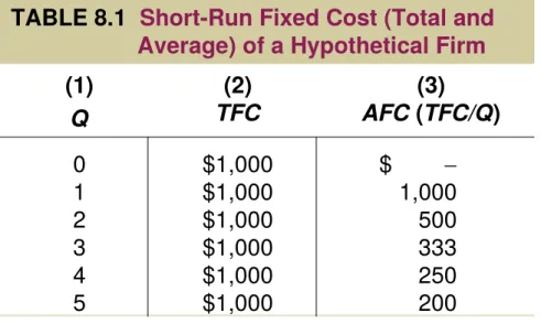
TABLE 8.1 Short-Run Fixed Cost (Total and Average) of a Hypothetical Firm (1)
Q
(2)
TFC AFC ((3)TFC/Q)
0 1 2 3 4 5 $1,000 $1,000 $1,000 $1,000 $1,000 $1,000 $ 1,000 500 333 250 200
COSTS IN THE SHORT RUN
total fixed costs (TFC) or overhead The
total of all costs that do not change with output, even if output is zero.
Total Fixed Cost (TFC)
FIXED COSTS
10 of 33
COSTS IN THE SHORT RUN
spreading overhead The process of dividing
total fixed costs by more units of output.
Average fixed cost declines as quantity rises.
11 of 33
COSTS IN THE SHORT RUN
(9 x $2) + (6 x $1) = $24 (6 x $2) + (14 x $1) = $26 6 14 9 6 A B
3 Units of output
(7 x $2) + (6 x $1) = $20 (4 x $2) + (10 x $1) = $18 6 10 7 4 A B
2 Units of output
4
6 (4 x $2) + (4 x $1) = $12(2 x $2) + (6 x $1) = $10 4
2
A B
1 Unit of output
TOTAL VARIABLE COST ASSUMING PK = $2, PL = $1
TVC = (K x PK) + (L x PL) USING
TECHNIQUE
UNITS OF INPUT REQUIRED
(PRODUCTION FUNCTION) K L PRODUCE
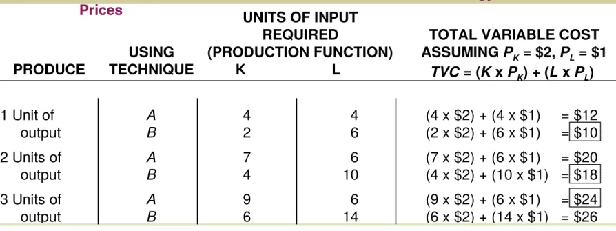
TABLE 8.2 Derivation of Total Variable Cost Schedule from Technology and Factor Prices
12 of 33
COSTS IN THE SHORT RUN
The total variable cost curve embodies information about both factor, or input, prices and technology. It shows the cost of production using the best available technique at each output level given current factor prices.
13 of 33
TABLE 8.3 Derivation of Marginal Cost from Total Variable Cost
UNITS OF OUTPUT TOTAL VARIABLE COSTS ($) MARGINAL COSTS ($)
0 1 2 3
0 10 18 24
0 10 8 6
COSTS IN THE SHORT RUN
Although the easiest way to derive marginal cost is to look at total variable cost and
subtract, do not lose sight of the fact that when a firm increases its output level, it hires or demands more inputs. Marginal cost measures the additional cost of inputs required to produce each successive unit of output.
marginal cost (MC) The increase in total cost that
14 of 33
COSTS IN THE SHORT RUN
The Shape of the Marginal Cost Curve in the Short Run
15 of 33
COSTS IN THE SHORT RUN
Graphing Total Variable Costs and Marginal Costs
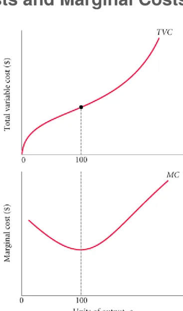
FIGURE 8.5 Total Variable Cost and Marginal Cost for a Typical Firm
MC TVC
TVC q
TVC
TVC
1 Δ
of slope
Average Variable Cost
(AVC)
q
TVC
16 of 33
COSTS IN THE SHORT RUN
Marginal cost intersects average variable cost at the lowest, or minimum, point of AVC.
Graphing Average Variable Costs and Marginal Costs
17 of 33
COSTS IN THE SHORT RUN
18 of 33
COSTS IN THE SHORT RUN
FIGURE 8.8 Average Total Cost = Average Variable Cost + Average Fixed Cost
The relationship between average total cost and marginal cost is
exactly the same as the
COSTS IN THE SHORT RUN
SHORT-RUN COSTS: A REVIEW
TABLE 8.5 A Summary of Cost Concepts
TERM DEFINITION EQUATION
Accounting costs Out-of-pocket costs or costs as an accountant would
define them. Sometimes referred to as explicit costs. Economic costs Costs that include the full opportunity costs of all inputs.
These include what are often called implicit costs. Total fixed costs Costs that do not depend on the quantity of output
produced. These must be paid even if output is zero. TFC Total variable costs Costs that vary with the level of output. TVC
Total cost The total economic cost of all the inputs used by a
firm in production. TC = TFC + TVC Average fixed costs Fixed costs per unit of output. AFC = TFC/q
Average variable costs Variable costs per unit of output. AVC = TVC/q
Average total costs Total costs per unit of output. ATC = TC/q ATC = AFC + AVC
Marginal costs The increase in total cost that results from
COSTS IN THE SHORT RUN
Marginal cost is the cost of one additional unit. Average variable cost is the total variable cost divided by the total number of units produced.
TABLE 8.4 Short-Run Costs of a Hypothetical Firm
(1)
q TVC(2)
(3)
MC
( TVC)
(4)
AVC
(TVC/q) TFC(5)
(6)
TC
(TVC + TFC)
(7)
AFC
(TFC/q)
(8)
ATC
(TC/q or AFC + AVC)
0 $ 0 $ $ $1,000 $ 1,000 $ $
1 10 10 10 1,000 1,010 1,000 1,010
2 18 8 9 1,000 1,018 500 509
3 24 6 8 1,000 1,024 333 341
4 32 8 8 1,000 1,032 250 258
5 42 10 8.4 1,000 1,042 200 208.4
21 of 33
LONG-RUN COSTS: ECONOMIES
AND DISECONOMIES OF SCALE
increasing returns to scale, or economies of
scale An increase in a firm’s scale of production
leads to lower costs per unit produced.
constant returns to scale An increase in a
firm’s scale of production has no effect on costs per unit produced.
decreasing returns to scale, or diseconomies
of scale An increase in a firm’s scale of
22 of 33
LONG-RUN COSTS: ECONOMIES
AND DISECONOMIES OF SCALE
INCREASING RETURNS TO SCALE
The Sources of Economies of Scale
Most of the economies of scale that immediately come to mind are technological in nature.
23 of 33
LONG-RUN COSTS: ECONOMIES
AND DISECONOMIES OF SCALE
FIGURE 9.5 A Firm Exhibiting Economies of Scale
long-run average cost curve (LRAC) A graph that
24 of 33
LONG-RUN COSTS: ECONOMIES
AND DISECONOMIES OF SCALE
CONSTANT RETURNS TO SCALE
Technically, the term constant returns means that the quantitative relationship between input and output stays constant, or the same, when output is increased.
25 of 33
LONG-RUN COSTS: ECONOMIES
AND DISECONOMIES OF SCALE
DECREASING RETURNS TO SCALE
26 of 33
LONG-RUN COSTS: ECONOMIES
AND DISECONOMIES OF SCALE
optimal scale of plant The scale of plant
that minimizes average cost.
TABLE 7A.1 Alternative Combinations of Capital (K) and Labor (L) Required to Produce 50, 100, and 150 Units of Output
QX = 50 QX = 100 QX = 150
K L K L K L
A B C D E 1 2 3 5 8 8 5 3 2 1 2 3 4 6 10 10 6 4 3 2 3 4 5 7 10 10 7 5 4 3
27 of 33
ISOQUANTS AND ISOCOSTS
28 of 33
Isoquant A graph
that shows all the combinations of capital and labor that can be used to produce a given amount of output.
29 of 33
FIGURE 7A.2 The Slope of an Isoquant Is Equal to the Ratio of MPL to MPK
Slope of isoquant:
K L
MP
MP
L
K
marginal rate of
technical substitution
FIGURE 7A.3 Isocost Lines Showing the
Combinations of Capital and Labor Available for $5, $6, and $7
FACTOR PRICES AND INPUT
COMBINATIONS: ISOCOSTS
isocost line A
graph that shows all the combinations of capital and labor
31 of 33
FIGURE 7A.4 Isocost Line Showing All Combinations of Capital and Labor Available for $25
Slope of isocost line:
FIGURE 7A.5 Finding the Least-Cost Combination of Capital and Labor to Produce 50 Units of Output
FINDING THE LEAST-COST TECHNOLOGY WITH ISOQUANTS AND ISOCOSTS
The firm will choose the combination of inputs that is least costly. The least costly way to produce any given level of output is indicated by the point of tangency between an isocost line and the isoquant
33 of 33
FIGURE 7A.6 Minimizing Cost of Production for qX = 50,
qX = 100, and qX = 150
K L K L
P
P
MP
MP
slope
of
isocost
isoquant
of
slope
K L K LP
P
MP
MP
THE COST-MINIMIZING EQUILIBRIUM CONDITION
At the point where a line is just tangent to a curve, the two have the same slope. At each point of tangency, the
following must be true:
Thus,
Dividing both sides by PL and multiplying both sides by
MPK, we get