R E S E A R C H A R T I C L E
Open Access
Selection and processing of calibration
samples to measure the particle
identification performance of the LHCb
experiment in Run 2
Roel Aaij
8, Lucio Anderlini
5, Sean Benson
8, Marco Cattaneo
7, Philippe Charpentier
7,
Marco Clemencic
7, Antonio Falabella
4, Fabio Ferrari
4, Marianna Fontana
7*, Vladimir Vava Gligorov
3,
Donal Hill
12, Tibaud Humair
11, Christopher Robert Jones
9, Oliver Lupton
7,10, Sneha Malde
12,
Carla Marin Benito
2, Rosen Matev
7, Alex Pearce
7, Anton Poluektov
1,10, Barbara Sciascia
6,
Federico Stagni
7, Ricardo Vazquez Gomez
7and Yanxi Zhang
7*Correspondence:
[email protected] 7European Organization for Nuclear Research (CERN), Meyrin, Switzerland
Full list of author information is available at the end of the article
Abstract
Since 2015, with the restart of the LHC for its second run of data taking, the LHCb experiment has been empowered with a dedicated computing model to select and analyse calibration samples to measure the performance of the particle identification (PID) detectors and algorithms. The novel technique was developed within the framework of the innovative trigger model of the LHCb experiment, which relies on online event reconstruction for most of the datasets, reserving offline reconstruction to special physics cases. The strategy to select and process the calibration samples, which includes a dedicated data-processing scheme combining online and offline
reconstruction, is discussed. The use of the calibration samples to measure the detector PID performance, and the efficiency of PID requirements across a large range of decay channels, is described. Applications of the calibration samples in data-quality
monitoring and validation procedures are also detailed.
Keywords: Experimental methods and data analysis methods, Data acquisition, Data analysis methods
Introduction
LHCb is a dedicated heavy flavour physics experiment at the LHC. Its main goal is to search for indirect evidence of new physics in CP-violating processes and rare decays of beauty and charm hadrons. Among other performance metrics, like excellent vertex resolution and good momentum and invariant-mass resolution, charged particle identi-fication (PID) distinguishing electrons, muons, pions, kaons and protons traversing the detector is essential in the LHCb physics programme. The required performances range from the per mille misidentification probability of hadrons as muons in the study of the rare B(d,s) → μ+μ− decays [1–7], to the sub percent precision, over a wide kinematic
range accurate, on the detector induced asymmetries for the ambitious programme of CP asymmetry measurements [8–11].
PID information is extensively used both in the trigger selection and in offline data analysis. This required the development of a dedicated computing model and a strategy to select suitable calibration samples, in order to measure the PID performance and assess systematic effects. A careful design of the computing model is strategical since, thanks to the variety and abundance of the calibration samples available at the LHC, the statistical uncertainty on the measured selection efficiencies is limited by the amount of computing resources allocated to the task rather than from irreducible experimental factors.
In “Detector” section, an overview of the LHCb detector is given, together with a summary of the PID calibration samples required in order to accomplish the physics goals of LHCb with Run 2 data (2015−2018). The article then focuses on the strategy to select and process PID calibration samples, including a description of the multivari-ate classifiers used to combine the response of calorimeters, RICH and muon system (“Global particle identification” section); the procedure to measure the PID performance using dedicated calibration samples, together with the techniques to determine the selec-tion efficiency on hundreds of different decay channels, relying on a small number of calibration samples (“Measuring PID performance” section); the dedicated data-processing scheme combining online and offline reconstruction (“Computing model for the calibration samples” section); and the applications of the calibration samples to data-quality monitoring and validation (“Data data-quality, monitoring and validation” section). A brief summary and outlook are given in “Conclusions” section. While this article discusses the calibration samples specifically for charged particle identification, the general com-puting model and selection strategy is also being applied to other calibration samples in Run 2, such as those for tracking calibration and neutral pion and photon PID.
Detector
The LHCb detector is a single-arm forward spectrometer covering the pseudorapidity range 2 < η < 5, designed for the study of particles containingborcquarks [12,13]. The detector includes a high-precision tracking system consisting of a silicon-strip ver-tex detector surrounding theppinteraction region [14], a large-area silicon-strip detector located upstream of a dipole magnet with a bending power of about 4 Tm, and three stations of silicon-strip detectors and straw drift tubes [15] placed downstream of the magnet. The tracking system provides a measurement of momentum,p, of charged par-ticles with a relative uncertainty that varies from 0.5% at low momentum to 1.0% at 200GeV/c. The minimum distance of a track to a primary vertex, the impact parameter, is measured with a resolution of (15+29/pT)μm, wherepTis the component of the momen-tum transverse to the beam, in GeV/c. Photons, electrons and hadrons are identified by a calorimeter system (CALO) consisting of scintillating-pad and preshower detectors, an electromagnetic calorimeter and a hadronic calorimeter. Different types of charged hadrons are distinguished using information from two ring-imaging Cherenkov (RICH) detectors [16]. Muons are identified by a system composed of alternating layers of iron and multiwire proportional chambers [17].
parameters are made available for the online reconstruction, used in the trigger selection. Online calibration is of such high quality that it is also used for offline reconstruction, ensuring consistency between online and offline.
The responses of the calorimeter, RICH, and muon systems, or their combinations, associated to each track in the reconstruction process are named for brevity PID variables. They can be used in selections to increase the signal purity of a sample, reducing the pro-cessing time devoted to the reconstruction of background events, often characterized by high multiplicity, and helping in fitting into the data storage constraints. Moreover they allow selections to avoid an explicit bias on quantities of physical interest, such as decay time [21,22].
The many contexts in which particle identification is exploited within the experiment and the difficulties in obtaining a perfect simulation for the PID detectors, motivate the development of techniques for measuring the PID performance in suitable PID calibra-tion samples. These samples are datasets collected by LHCb where decay candidates have a kinematic structure that allows unambiguous identification of one of the daughters, without the use of any PID information from the calorimeter, RICH, or muon systems, so that they are unbiased from the particle identification point of view. Today, most LHCb physics analyses rely on calibration samples for the determination of PID efficiencies. In addition, these samples can be used to monitor time variations in performance, and to test new reconstruction algorithms.
The majority of physics analyses using data collected with the LHCb experiment rely on the physics quantities as reconstructed in the online trigger reconstruction. Still, physics analyses with special needs in terms of event reconstruction, searching for example for interactions of light nuclei or particles beyond the Standard Model with the detec-tor [23], are able to reprocess offline the collected calibration datasets with dedicated reconstruction algorithms.
In order to enable the measurement of selection efficiencies that combine trigger requirements on the online-computed PID variables and offline requirements of PID variables obtained through dedicated reconstruction algorithms, an innovative dedi-cated data-processing strategy has been designed. Calibration data are obtained through a real-time selection based on the online reconstruction without any requirement on PID variables. Each event belonging to the calibration samples is fully reconstructed independently both online and offline. The resulting reconstructed particles are then matched, allowing a measurement of the efficiency of requirements that combine the two reconstruction types as described in “Measuring PID performance” section.
Global particle identification
The reconstruction algorithms of each of the PID detectors of the LHCb experiment are very different, but each of them allows the computation of a likelihood ratio between particle hypotheses for each reconstructed track [13]. The reconstruction algorithm of the RICH detectors provides the likelihood of the electron, muon, kaon, proton and deuteron hypotheses relative to the pion hypothesis. The calorimeter system provides the likelihood of electrons relative to the pion hypothesis. Finally, the muon system provides the likelihoods of the muon and non-muon hypotheses. The likelihood ratios of the three detector systems are combined intoCombined Differential Log-Likelihoods
Selection strategies based on CombDLL and isMuon [24], a binary variable loosely identifying muons, are widely employed already at the trigger level [25].
Following recent developments in machine learning, more advanced classifiers have also been designed to combine the likelihoods ratios defined above with the informa-tions from the tracking system, including the kinematic variables of the particle, and additional information from the PID detectors not entering the likelihood computa-tion (e.g. the number of hits in the muon system shared among reconstructed tracks). The classifier with the widest application in this category, namedANNPID, was devel-oped usingForward Feeding Artificial Neural Networks[26], structured as aMulti-Layer Perceptron (MLP) with a single hidden layer composed of roughly 20% more nodes than the input layer activated, through a sigmoid function. The network is trained minimizing the Bernoulli Cross-Entropy with Stochastic Gradient Descent as imple-mented in the TMVA package [26]. Bernoulli Cross-Entropy originated from information theory and is proportional to the likelihood of a perfect binary classification of the training sample [27]. Alternative implementations and training strategies are also being developed [28], but their treatment falls outside the scope of this paper. The train-ing sample is obtained from abundant simulated decays of heavy hadrons that emulate the kinematic distributions of signal samples studied in several analyses. Depending on the arrangement of the input samples, on the quality of the simulation, and on the available number of simulated events, the response of the ANNPID algorithm can vary. As a consequence, the response of the ANNPID algorithms is provided in sev-eral tunings, some for gensev-eral purpose, and others specialised for a particular analysis or kinematic range. The variables combined using the ANNPID classifiers are listed in Table1.
All of the input variables for the ANNPID classifiers are made immediately available to physics analyses, easing the development of new tunings and classification algorithms dedicated to single analyses. The many output variables of the detector reconstruction which are not used as input to ANNPID can be accessed or even regenerated, relying on the raw detector data stored on tape.
Measuring PID performance
More than twenty exclusive trigger selections are designed to select pure samples of the five most common charged particle species that interact with the LHCb detector: pro-tons, kaons, pions, muons and electrons [29]. Generally, low-multiplicity decay modes with large branching fractions are chosen in order to enhance the statistics and the purity and populate the tails in the distributions of the PID variables, which are of great rel-evance when computing misidentification probabilities. Completely reconstructed final states composed of charged particles only are preferred, as they are selected with high purity at LHCb. An overview of the modes utilised is given in Table2.
Table 1Input variables of the ANNPID classifiers for the various subsystems of the LHCb detector
Tracking
Total momentum Transverse momentum Quality of the track fit
Number of clusters associated to the track
ANN response trained to reject ghost tracks [42]
Quality of the fit matching track segments upstream and downstream of the magnet
RICH detectors
Geometrical acceptance of the three radiators, depending on the direction of the track Kinematical acceptance due to Cherenkov threshold for muons and kaons
Likelihood of the electron, muon, kaon, and proton hypotheses relative to the pion Likelihood ratio of the below-threshold and pion hypotheses
Electromagnetic calorimeter
Likelihood ratio of the electron and hadron hypotheses
Likelihood ratio of the muon and hadron hypotheses
Matching of the track with the clusters in thepreshowerdetector
Likelihood ratio of the electron and pion hypotheses, after recovery of the Bremsstrahlung photons
Hadronic calorimeter
Likelihood ratio of the electron and hadron hypotheses
Likelihood ratio of the muon and hadron hypotheses
Muon system
Geometrical acceptance
Loose binary requirement already available in the hardware trigger
Likelihood of the muon hypothesis Likelihood of the non-muon hypothesis
Number of clusters associated to at least another track
In order to avoid a pre-selection that biases the PID variables, the selection strategy of the calibration samples imposes requirements on the algorithms selecting the event in the previous trigger layers. Either the trigger algorithms do not rely on PID information, or the PID selection in the trigger is applied to one of the particles not used to measure the performance.
Several of the selection strategies are implemented according to the so-called tag-and-probemodel [17]. Taking theJ/ψ → μ+μ−decay as an example, - the tag-and-probe selection strategy relies on a list of well-identified tag muons of a certain charge and a list of probe tracks with opposite charge, selected avoiding any PID requirement. These are combined to form muon pairs with invariant-mass consistent with theJ/ψmass, and
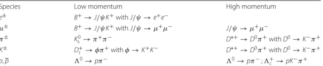
Table 2Overview of decay modes that are used to select calibration samples
Species Low momentum High momentum
e± B+→J/ψK+withJ/ψ→e+e−
μ± B+→J/ψK+withJ/ψ→μ+μ− J/ψ→μ+μ−
π± K0
s →π+π− D∗+→D0π+withD0→K−π+
K± D+s →φπ+withφ→K+K− D∗+→D0π+withD0→K−π+
p,p 0→pπ− 0→pπ−;+
c →pK−π+
are then filtered further on the basis of the quality of the fit of the decay vertex, to form the final sample. To extend thepTrange of the muons in the calibration samples to lower values, where the background from low momentum pions is difficult to reduce, theJ/ψ
candidates can be combined with charged kaons to form B+ → J/ψK+ candidates1, adding further kinematic constraints related to theBdecay to the final filtering.
Proton calibration samples are obtained from two different decay modes:0 → pπ− and+c → pK−π+. Since the visible 0 production cross section in LHCb is several orders of magnitude larger with respect to heavy flavour production, the yield collected at the trigger level exceeds the needs in terms of statistical precision on the particle identi-fication. This would pose severe challenges for data storage. Therefore, a large fraction of these signal candidates is discarded by running the selection only on a randomly selected fraction of the events. In order to improve the kinematic coverage of the sample, the fraction of discarded events is defined differently in four bins of the proton transverse momentum(pT), resulting in a higher retention rate in the less-populated high-pTregion. The sample of+c decays is included to extend thepTcoverage of the0samples.
An abundant calibration sample for pions is provided by the decayKs0→π+π−, but the spectrum of the probe particles is much softer than what is typical for hadrons produced in heavy hadron decays. Charm hadron decays allow the kinematic range to be extended to higher transverse momenta, but the lower purity of the samples, due to the smaller production cross-section, requires additional care in the selection and background sub-traction strategies. The decayD∗+ → D0π+withD0 → K−π+represents the primary source ofπ±andK±calibration samples. The soft pion produced in the strong decay of theD∗+hadron allows to tag the flavour of theD0and therefore to distinguish the kaon and the pion produced in its decay without PID requirements on either of the two probe particles. Applying a requirement on the energy release in theD∗+→D0π+decay, which is expected to be small, enables the rejection of combinatorial background due to the erro-neous combination ofD0hadrons and pions produced in unrelated processes. Finally, the
D+s →φπ+decay withφ →K+K−is a further source of kaons. This sample allows the kinematic range for kaons to be extended to lower momenta, as theφconstraint enables the kinematic requirements on the kaons to be loosened while retaining the purity.
The residual background that cannot be rejected with an efficient selection strategy is statistically subtracted assigning a signed weight (namedsWeight) to each decay
candi-date, as prescribed by thesPlot technique [30]. A fit to the invariant-mass of the decaying
particle is performed for each calibration sample, defining a signal component for which the sample of probe tracks is known to be pure, and one or more background compo-nents of different nature. In several cases, two-dimensional fits are performed to account for additional background sources. The variables used in the two-dimensional fits are: the
D0mass andD∗+ −D0mass difference forD∗+ → D0π+; theB+andJ/ψ masses for
B+→J/ψ →μ+μ−K+; theφandD+s masses forD+s →φπ+.
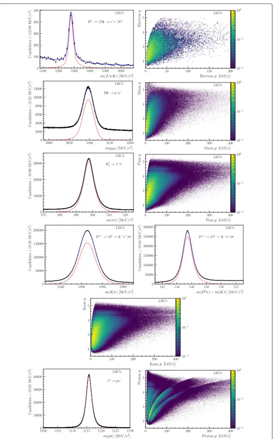
the chosen discriminating variables and the PID variables do not play a significant role. Figure1illustrates the invariant-mass distributions for some of the calibration samples, as obtained from proton-proton collision data collected in 2015 corresponding to an integrated luminosity of 0.17 fb−1. The corresponding kinematic distributions for the different species of probe particles are also shown.
The performance of the PID detectors to a traversing particle depends on the kinemat-ics of the particle, the occupancy of the detectors (which may be different event-to-event and for different particle production mechanisms), and experimental conditions such as alignments, temperature, and gas pressure (which may modify the response of detectors across runs).
One may assume that the response of a PID variable is fully parameterised by some known set of variables, such as the track momentump(which is related to the Cherenkov angle in the RICH and to the energy deposited in the calorimeter) and the track multi-plicity, the latter being given by the number of reconstructed tracks traversing the whole detector. By partitioning the sample with sufficient granularity in these parameterising variables, the PDF of the PID variable distribution does not vary significantly within each subset, such that the efficiency of a selection requirement on that variable is constant within each subset [40].
In the trivial case of events that come from the calibration sample, there is no need to compute per-subset efficiencies, and the average efficiency is simply given by the fraction of background subtracted events passing the PID requirement. To compute the PID effi-ciency on a sample other than the calibration sample, denoted hereafter as thereference sample, the parameterising variables in the calibration sample can be weighted to match those in the reference sample. The PID efficiency can then be computed using the per-subset weights. The weights are defined as the normalised ratio of reference to calibration tracks
wi=
Ri
Ci ×
C
R , (1)
whereRi(Ci) is the number of reference (calibration) tracks in theith subset, andR(C) is
the total number of reference (calibration) tracks in the sample.
After applying the PID cut to the weighted calibration sample, the average efficiency of the PID requirement on the weighted calibration sample is
¯
ε=
iεiwiCi
iwiCi
. (2)
wherewiis the per-subset weight,iis the per-subset efficiency andCiis the number of
calibration tracks in thei-th subset.
The computation of the PID efficiency can be thought of as the reweighting of the cal-ibration sample to match the reference, or as the assignment of efficiencies to reference tracks based on the subset they belong to. This can also be extended to reference sam-ples where PID requirements have been imposed on multiple tracks, where the efficiency of an ensemble of cuts is required taking into account the kinematic correlation between tracks.
Fig. 1On the left, mass distributions of the decaying particles with the results of the fit superimposed; signal contributions are shown by the red dashed curves, and the total fit functions including background contributions are shown by the blue solid curves. On the right, the background-subtracted distributions of the calibration samples for electrons, muons, pions, kaons and protons as a function of the track
signal tracks under consideration. This is an ideal approach to use when the kinematics of the signal tracks are known to be well modelled in the simulation. If the signal in data can be reliably separated from the other species in the sample, such that some background subtraction can be used to extract the signal kinematics, a second approach to creating the reference sample can be used.
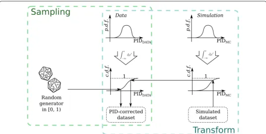
Lastly, the PID response of MC signal samples can be corrected using the PID calibration data samples. Two options are provided:
• Resampling of PID variables, where the PID response is completely replaced by the one statistically generated from calibration PDFs.
• Transformation of PID variables, where the PID variables from the simulation are transformed such that they are distributed as in data.
The PID correction is still considered as a function of track kinematics (pTandη) and event multiplicityNevt (such as the number of tracks in the event). However, unlike in the first two strategies detailed above, the correction is performed using an unbinned approach, where the calibration PDFs in four dimensions, the PID variable,pT,η, and a measure ofNevt, are described by a kernel density estimation procedure using the Meerkat library [31]. The advantage of resampling and variable transformation is that the corrected PID response can be used as an input to a multivariate classifier.
However, a limitation of the PID resampling approach is that the PID variables for the same track are generated independently, and thus no correlations between them are reproduced. Therefore, only one PID variable per track can be used in the selection. Cor-relations between variables for different tracks are preserved via corCor-relations with the kinematics of tracks, assuming the PID response is fully parameterised bypT,η, andNevt. The PID variable transformation approach aims to remove this limitation [32]. The corrected PID variable PIDcorris obtained as
PIDcorr=P−1exp(PMC(PIDMC|pT,η,Nevt)|pT,η,Nevt), (3)
wherePMC(PIDMC|pT,η,Nevt)is the cumulative distribution function of the simulated PID variable PIDMC, andP−1exp(x|pT,η,Nevt)(where 0< x<1) is the inverse cumulative distribution function for the PID variable from the calibration sample (i.e. for fixedpT,η andNevtit returns the PID variable that corresponds to a cumulative probabilityx). The functions are obtained from the results of kernel density estimations of the simulation and calibration PID responses, respectively. The corrected PID variables obtained in this way follow the PDF of the calibration sample, but preserve strong correlations with the output of simulation. Through these correlations in simulation, the ones between PID variables for the same track are reproduced to first order. The drawback of this approach is that it also relies on the parametrisation of PID PDFs in simulation, which are extracted from samples that are typically much smaller than the calibration data. Although one naively expects this method to perform better due to taking correlations into account, studies are ongoing to quantify the degree of agreement between the correlations found in simulation and data. The PID resampling and variables transformation techniques are schematically represented in Fig.2.
Fig. 2Schematic representation of the PID resampling and variable transformation techniques
large calibration sample sizes, this uncertainty is usually dominated by the size of the signal reference sample.
Several sources of systematic uncertainty related to the procedure must also be accounted for, arising from differences between the reference and signal samples, the spe-cific choice of binning used, and thesWeight procedure used in the calibration sample
production. The degree to which these uncertainties affect the PID efficiency precision is analysis dependent, and require specific studies to be carried out on a case-by-case basis. Moreover the availability of primary and secondary calibration samples allows to study possible biases coming from single decay modes.
Computing model for the calibration samples
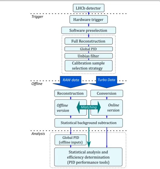
In order to face the new challenges of the second run of the LHC, the LHCb trigger [33,34] has evolved into a heterogeneous configuration with different output data for-mats for different groups of trigger selections. Figure3shows a schematic representation of the computing model that is described in the following.
Two alternative data formats for physics analyses, namedTurbostream [35] andFull stream, have been developed. Trigger selections writing to theTurbostream are intended for analyses of samples where only the information related to the candidates and associ-ated reconstructed objects is needed. Trigger selections that are part of the Turbo stream produce a decay candidate which is stored for offline analysis, along with a large number of detector-related variables, while the raw detector data is not kept [35,36]. When con-sidering analyses based on theTurbostream, it is therefore evident that the calibration samples must provide the PID information as computed online in order to assess the effi-ciency of selection requirements applied either in the trigger selection, or offline on the PID variables retrieved from the trigger candidate.
Fig. 3Schematic representation of the computing model for the PID calibration samples
in the trigger decision. The track and decay candidates are reproduced in a further offline reconstruction step that accesses the raw detector data. Indeed, some physics data anal-yses present special needs in terms of particle identification algorithms, for example because they explore kinematic regions at the boundaries of the kinematic acceptance, or because of exceptional requirements in terms of the accuracy of the efficiency determi-nation. To respond to such special requirements, dedicated algorithms accessing the raw detector data can be developed and included in the offline event reconstruction. Hence, the events selected as part of the calibration samples must include the raw data, allowing the performance of future algorithms to be measured on data.
multivariate classifiers adopted in the trigger and in the statistical data analysis, require the use of calibration samples combining the information from the online and offline reconstruction, allowing full offline reprocessing if needed.
A dedicated data format, namedTurboCalib, was developed to satisfy the require-ments on PID calibration samples described above [37]. After the online full event reconstruction, events in which decay candidates useful for calibration are identified and selected in real-time are stored including both the trigger candidates themselves and raw detector data. The two output formats are processed independently for each event, to obtain both decay candidates propagated from the trigger and decay candi-dates reconstructed offline from the raw detector data. The two reconstructions are fully independent, so that the tracks identified in the two processes must be matched. This is done according to the fraction of shared clusters in the detector, or exploiting the TisTos algorithm described in Ref. [38], or with a combination of the two techniques.
The offline versions of the PID variables can be easily replaced with other tunings of the multivariate classifiers, or through the output of dedicated reconstruction sequences. As a result of the matching procedure, each reconstructed track is associated to two sets of PID variables, obtained through the online and offline versions of the reconstruction, respec-tively. The two sets are available to the analysts to measure the efficiency of selection requirements that possibly combine the two versions.
As described in “Measuring PID performance” section, the measurement of the selec-tion efficiencies from the selected calibraselec-tion samples is enabled through the subtracselec-tion of the residual background by means of thesPlot technique. In order to overcome to
the scalability challenges set by the increasing needs for precision in many LHCb mea-surements, resulting in huge calibration samples to control the statistical uncertainty, the background subtraction is performed through a dedicated, distributed implementation of thesPlot technique. Finely binned histograms of the invariant-mass distributions of
the trigger candidates are filled in parallel on thousands of computing nodes. They are then merged and modeled through a maximum likelihood fit as the combination of signal and background components. The relations between the discriminating variables and the
sWeights to be assigned to each candidate are sampled in fine grids and made available
through a distributed file system to the computing nodes of the LHCb grid [39], where jobs to assign the weights are run as a final processing step in the calibration sample pro-duction workflow. Such a distributed implementation of thesPlot technique avoids the
storage of the entire dataset on a single computing node, hence scaling better with the size of the calibration samples.
The real-time selection strategy, the double-processing scheme combining event-by-event the online and offline reconstructed variables, and the distributed approach to background subtraction constitute the main novelties in the data processing for the cali-bration samples, overcoming most scalability issues and making the limited cross-section and the available data storage resources the only limitations to the statistical precision in the determination of PID selection efficiencies.
of variables identifying the kinematics of the tracks, the event multiplicity and the PID response can be chosen case by case, while the access to calibration samples and the implementation of the algorithms are maintained centrally.
Data quality, monitoring and validation
As discussed in “Measuring PID performance” section, calibration samples are abundant decays with high purity which are selected at the trigger level. They are represen-tative of all the families of long-lived charged particles interacting with the LHCb detector, apart from deuterons. Their immediate availability during the data taking and their high statistics are key ingredients for data-quality monitoring and vali-dation. Since the reconstruction involves different systems of the LHCb detectors depending on the nature of the particle, the various samples are used to monitor and validate different aspects of the reconstruction. For example, the recovery of Bremsstrahlung photons to improve the momentum resolution of the electrons can only be monitored and validated using an electron sample. Similarly, the efficiency of muon identification can be better monitored and validated using a sample of tagged muons.
In order to add redundancy to the validation procedure, a small fraction of the cali-bration samples are reconstructed with the offline procedure in real time. This enables alarms to be triggered when misalignments occur between the online and offline recon-struction, due to errors in the database handling the alignment and calibration constants, for example.
Finally, several checks on the reconstructed quantities in the calibration samples have been included in the automated validation procedure performed during data taking. These aim to identify deviations from standard running conditions, and check for pos-sible temporal variations in performance due to unstable environmental conditions, or ageing of the detector [41].
Real-time monitoring on pure decay samples representative of the needs of a wide physics programme will be of critical importance during Run 3 of the LHC, when, after a major upgrade of the LHCb experiment, most datasets to perform physics data analy-ses will be selected in the trigger and stored as decay candidates, with no support for raw detector data [36]. Since no further reprocessing of the reconstruction will be possible, any loss in performance will unavoidably result in a loss of effectiveness for the resulting physics measurements.
Conclusions
The strategy to select and process the calibration samples used to measure the PID per-formance has seen several improvements to face the challenges set by Run 2 of the LHC. The samples are now selected directly in real-time at the highest level of the software trig-ger, introducing an important benefit in terms of statistics and absence of selection bias with respect to the offline selection strategy adopted in Run 1. The calibration samples are used to measure the PID performance, to correct the simulated samples, and to monitor the detector performance during the data-taking.
The new scheme has been later adopted to provide the tracking and the photon reconstruction performance, paving the way for Run 3.
Endnote
1Charged-conjugated candidates are implicitly considered here and throughout the
paper.
Abbreviations
CALO: Calorimeter; CombDLL: Combined Differential Log-Likelihoods; MLP: Multi-Layer Perceptron; PID: Particle identification; RICH: Ring-imaging Cherenkov
Acknowledgements
We express our gratitude to our colleagues in the CERN accelerator departments for the excellent performance of the LHC. We thank the technical and administrative staff at the LHCb institutes. We acknowledge support from CERN and from the national agencies: CNRS/IN2P3 (France); INFN (Italy); NWO (The Netherlands); MinECo (Spain); SNSF and SER (Switzerland); STFC (United Kingdom); We acknowledge the computing resources that are provided by CERN, IN2P3 (France), INFN (Italy), SURF (The Netherlands), PIC (Spain), GridPP (United Kingdom), CSCS (Switzerland). We are indebted to the communities behind the multiple open-source software packages on which we depend.
Funding
CERN, The European Organization for Nuclear Research (Switzerland), Istituto Nazionale di Fisica Nucleare (INFN), Nederlandse Organisatie voor Wetenschappelijk Onderzoek (NWO), SURF, Collaborative organisation for ICT in Dutch higher education and research, Conseil Général de Haute-Savoie, ANR. Agence Nationale de la Recherche, Labex P2IO, Physique des 2 Infinis et des Origines, Labxx ENIGMASS, L’enigme de la Masse, Labex OCEVU, Origine Constituants et Evolution de l’Univers, Région Auvergne-Rhone-Alpes, Herchel Smith Fund, The Royal Society, The Royal Commission for the Exhibition of 1851, English-Speaking Union, Leverhulme Trust, Generalitat de Catalunya, PIC, Port d’Informacio Cientifica
Availability of data and materials
Data will not be available immediately but it will be shared in the future, according to the following policyhttp:// opendata.cern.ch/record/410
Authors’ contributions
Rj (Sec. 2, 5), LA (Sec. 1, 2, 3, 4, 5), SB (Sec. 2, 5), MC (Sec. 2, 5), PC (Sec. 2, 5), MC (Sec. 2, 5), AF (Sec. 2, 5), FF (Sec 2, 4, 6), MF (Sec. 1, 2, 3, 4, 5), VVG (Sec. 2, 5), DH (Sec. 1, 2, 3, 4, 5), TH (Sec 2, 4, 6), CRJ (Sec 2, 3), OL (Sec 4, 6), SM (Sec 4, 6), CMB (Sec 4, 6), RM (Sec. 2, 5), AP (Sec. 2, 5), AP (Sec. 2, 4), BS (Sec. 1, 2, 3, 4, 7), FS (Sec. 2, 5), RVG (Sec. 2, 4, 6), Y-XZ (Sec. 2, 4). All authors read and approved the final manuscript.
Ethics approval and consent to participate Not applicable.
Consent for publication Not applicable.
Competing interests
The authors declare that they have no competing interests.
Publisher’s Note
Springer Nature remains neutral with regard to jurisdictional claims in published maps and institutional affiliations.
Author details
1Aix Marseille Univ, CNRS/IN2P3, CPPM, Marseille, France.2LAL, Université Paris-Sud, CNRS/IN2P3, Université Paris-Saclay,
Orsay, France.3Université Pierre et Marie Curie, Université Paris Diderot, CNRS/IN2P3, Paris, France.4Istituto Nazionale di
Fisica Nucleare, Sezione di Bologna, Bologna, Italy.5Istituto Nazionale di Fisica Nucleare, Sezione di Firenze, Florence, Italy. 6Istituto Nazionale di Fisica Nucleare, Laboratori Nazionali di Frascati, Frascati, Italy.7European Organization for Nuclear
Research (CERN), Meyrin, Switzerland.8Nikhef, Amsterdam, Netherlands.9University of Cambridge, Cambridge, United
Kingdom.10Department of Physics, University of Warwick, Coventry, United Kingdom.11Imperial College London,
London, United Kingdom.12University of Oxford, Oxford, United Kingdom.
Received: 24 August 2018 Accepted: 1 February 2019
References
1. Aaij R, et al (2011) Search for the rare decaysB0
s→μ+μ−andB0→μ+μ−. Phys Lett B699:330.https://doi.org/10.
1016/j.physletb.2011.04.031.1103.2465
2. Aaij R, et al (2012) Search for the rare decaysB0s→μ+μ−andB0→μ+μ−. Phys Lett B708:55.https://doi.org/10.
1016/j.physletb.2012.01.038.1112.1600
3. Aaij R, et al (2012) Strong constraints on the rare decaysB0
s→μ+μ−andB0→μ+μ−. Phys Rev Lett 108:231801.
https://doi.org/10.1103/PhysRevLett.108.231801.1203.4493
4. Aaij R, et al (2013) First evidence for the decayB0
s→μ+μ−. Phys Rev Lett 110:021801.https://doi.org/10.1103/
5. Aaij R, et al (2013) Measurement of theB0
s→μ+μ−branching fraction and search forB0→μ+μ−decays at the
LHCb experiment. Phys Rev Lett 111:101805.https://doi.org/10.1103/PhysRevLett.111.101805.1307.5024
6. Khachatryan V, et al (2015) Observation of the rareB0s →μ+μ−decay from the combined analysis of CMS and
LHCb data. Nature 522:68.https://doi.org/10.1038/nature14474.1411.4413
7. Aaij R, et al (2017) Measurement of theB0
s→μ+μ−branching fraction and effective lifetime and search for
B0→μ+μ−decays. Phys Rev Lett 118:191801.https://doi.org/10.1103/PhysRevLett.118.191801.1703.05747
8. Aaij R, et al (2013) Measurement of the CKM angleγfrom a combination ofB±→Dh±analyses. Phys Lett B726:151.https://doi.org/10.1016/j.physletb.2013.08.020.1305.2050
9. Aaij R, et al (2014) Measurement ofCPviolation and constraints on the CKM angleγinB±→DK±with
D→K0
sπ+π−decays. Nucl Phys B888:169.https://doi.org/10.1016/j.nuclphysb.2014.09.015.1407.6211
10. Aaij R, et al (2014) Measurement of the CKM angleγusingB±→DK±withD→K0
sπ+π−,Ks0K+K−decays.
JHEP 10:097.https://doi.org/10.1007/JHEP10(2014)097.1408.2748
11. Aaij R, et al (2017) Measurement ofCPobservables inB±→D(∗)K±andB±→D(∗)π±decays. Phys Lett B777:16.
https://doi.org/10.1016/j.physletb.2017.11.070.1708.06370
12. Alves Jr. AA, et al (2008) The LHCb detector at the LHC. JINST 3:08005.https://doi.org/10.1088/1748-0221/3/08/ S08005
13. Aaij R, et al (2015) LHCb detector performance. Int J Mod Phys A30:1530022.https://doi.org/10.1142/ S0217751X15300227.1412.6352
14. Aaij R, et al (2014) Performance of the LHCb Vertex Locator. JINST 9:09007.https://doi.org/10.1088/1748-0221/9/09/ P09007.1405.7808
15. Arink R, et al (2014) Performance of the LHCb Outer Tracker. JINST 9:01002.https://doi.org/10.1088/1748-0221/9/01/ P01002.1311.3893
16. Adinolfi M, et al (2013) Performance of the LHCb RICH detector at the LHC. Eur Phys J C73:2431.https://doi.org/10. 1140/epjc/s10052-013-2431-9.1211.6759
17. Alves Jr. AA, et al (2013) Performance of the LHCb muon system. JINST 8:02022.https://doi.org/10.1088/1748-0221/ 8/02/P02022.1211.1346
18. Aaij R, et al (2013) The LHCb trigger and its performance in 2011. JINST 8:04022.https://doi.org/10.1088/1748-0221/ 8/04/P04022.1211.3055
19. Dujany G, Storaci B (2015) Real-time alignment and calibration of the LHCb Detector in Run II.https://cds.cern.ch/ record/2017839
20. Frank M, Gaspar C, Jost B, Neufeld N (2015) The LHCb Data Acquisition and High Level Trigger Processing Architecture. J Phys Conf Ser 664(8):082011
21. Aaij R, et al (2014) Measurement of theB+c meson lifetime usingB+c →J/ψμ+νμXdecays. Eur Phys J C74:2839.
https://doi.org/10.1140/epjc/s10052-014-2839-x.1401.6932
22. Aaij R, et al (2014) Measurements of theB+,B0,B0
smeson and0bbaryon lifetimes. JHEP 04:114.https://doi.org/10.
1007/JHEP04(2014)114.1402.2554
23. Aaij R, et al (2015) Search for long-lived heavy charged particles using a ring-imaging Cherenkov technique at LHCb. Eur Phys J C75:595.https://doi.org/10.1140/epjc/s10052-015-3809-7.1506.09173
24. Archilli F, et al (2013) Performance of the muon identification at LHCb. JINST 8:10020. https://doi.org/10.1088/1748-0221/8/10/P10020.1306.0249
25. Archilli F, et al (2013) Performance of the Muon Identification at LHCb. JINST 8:10020. https://doi.org/10.1088/1748-0221/8/10/P10020.1306.0249
26. Hoecker A, Speckmayer P, Stelzer J, Therhaag J, von Toerne E, Voss H (2018). J Phys Conf Ser 1085(4):042038.https:// doi.org/10.1088/1742-6596/1085/4/042038
27. Goodfellow I, Bengio Y, Courville A (2016) Deep Learning. MIT Press.http://www.deeplearningbook.org
28. Derkach D, Hushchyn M, Likhomanenko T, Rogozhnikov A, Kazeev N, Chekalina V, Neychev R, Kirillov S, Ratnikov F (2018) Ratnikov: Machine-Learning-based global particle-identification algorithms at the LHCb experiment. J Phys Conf Ser 1085(4):042038.https://doi.org/10.1088/1742-6596/1085/4/042038
29. Lupton O, Anderlini L, Sciascia B, Gligorov V (2016) Calibration samples for particle identification at LHCb in Run 2. Technical Report LHCb-PUB-2016-005. CERN-LHCb-PUB-2016-005, CERN, Geneva.https://cds.cern.ch/record/ 2134057
30. Pivk M, Le Diberder FR (2005) sPlot: A statistical tool to unfold data distributions. Nucl Instrum Meth A555:356–69.
https://doi.org/10.1016/j.nima.2005.08.106.physics/0402083
31. Poluektov A (2015) Kernel density estimation of a multidimensional efficiency profile. JINST 10(02):02011.https://doi. org/10.1088/1748-0221/10/02/P02011.1411.5528
32. Tanabashi M, et al (2018) Review of Particle Physics. Phys Rev D 98:030001.https://doi.org/10.1103/PhysRevD.98. 030001
33. Aaij R, et al (2013) The LHCb Trigger and its Performance in 2011. JINST 8:04022.https://doi.org/10.1088/1748-0221/ 8/04/P04022.1211.3055
34. Albrecht J, Gligorov VV, Raven G, Tolk S (2014) Performance of the LHCb High Level Trigger in 2012. J Phys Conf Ser 513:012001.https://doi.org/10.1088/1742-6596/513/1/012001.1310.8544
35. Aaij R, et al (2016) Tesla: an application for real-time data analysis in High Energy Physics. Comput Phys Commun 208:35–42.https://doi.org/10.1016/j.cpc.2016.07.022.1604.05596
36. Aaij R, et al (2014) LHCb Trigger and Online Upgrade Technical Design Report CERN-LHCC-2014-016. LHCB-TDR-016.
https://cds.cern.ch/record/1701361
37. Anderlini L, Benson S, Lupton O, Sciascia B, Gligorov V (2016) Computing strategy for PID calibration samples for LHCb Run 2. Technical Report LHCb-PUB-2016-020. CERN-LHCb-PUB-2016-020, CERN, Geneva.https://cds.cern.ch/ record/2199780
39. Stagni F, Tsaregorodtsev A, Arrabito L, Sailer A, Hara T, Zhang X, consortium D (2017) DIRAC in Large Particle Physics Experiments. J Phys Conf Ser 898(9):092020
40. Anderlini L, Contu A, Jones CR, Malde SS, Muller D, Ogilvy S, Otalora Goicochea JM, Pearce A, Polyakov I, Qian W, Sciascia B, Vazquez Gomez R, Zhang Y (2016) The PIDCalib package. Technical Report LHCb-PUB-2016-021. CERN-LHCb-PUB-2016-021, CERN, Geneva.https://cds.cern.ch/record/2202412
41. Adinolfi M, Archilli F, Baldini W, Baranov A, Derkach D, Panin A, Pearce A, Ustyuzhanin A (2017) Lhcb data quality monitoring. J Phys Conf Ser 898(9):092027