Sensitivity Analysis for Data Mining

Sensitivity Analysis for Data Mining

J. T. Yao

Department of Computer Science

University of Regina

Regina, Saskatchewan

Canada S4S 0A2

E-mail:

[email protected]

Abstract

An important issue of data mining is how to transfer data into information, the information into action, and the action into value or profit. This paper presents a study on applying sensitivity analysis to neural network models for a particu-lar area in data mining, interesting mining and profit min-ing. Applying sensitivity analysis to neural network mod-els rather than just regression modmod-els can help us identify sensible factors that play important roles to dependent vari-ables such as total profit in a dynamic environment.

1

Introduction

Data mining, as well as its synonyms knowledge discov-ering and information extraction, is frequently referred to the literature as the process of extracting interesting infor-mation or patterns from large databases [5, 6]. There are two major issues in data mining research and applications: patterns and interest. The techniques of pattern discovering include classification, association and clustering. Interest refers to patterns in business applications being useful or meaningful. Data mining may also be viewed as the pro-cess of turning the data into information, the information into action, and the action into value or profit [1, 12]. As summarized by Brijs et al. [2], there are three different lev-els of research tracks to study the interestingness of rules in data mining. Other than general measures and domain specific measures, an important measure of the interesting-ness is whether it can be used in the decision making pro-cess of a business to increase its profit. Recent research [2, 10, 11, 16, 18] focuses more on the later part of the process. However, little research appeared in literature that studies profit mining in a dynamic environment.

Sensitivity analysis methods estimate the rate of change in the output of a model,which is caused by the changes of the model inputs. They may be used to determine which

input parameter is more important or sensible to achieve ac-curate output values [15]. Sensitivity analysis has been ap-plied in various fields including complex engineering sys-tems, economics, physics, social sciences, medical decision making, risk assessment and many others [3, 4]. In the case of data mining, we may apply sensitivity analysis to find items that are sensible to total profit. These techniques al-low us not only to mine these patterns and rules that can lead to profit or actions but also to maximize profit in a dynamic environment. The aim of this paper is to identify the po-tential usefulness of sensitivity analysis techniques in data mining. In particular, we intend to show that by applying sensitivity analysis to neural network models, we can iden-tify sensible factors that play important roles to total profit and other dependent variables .

The organization of this paper is as follows. First, we present the motivation of this research in the next section. The second section also reviews recent relative work that has appeared the literature. The third and fourth sections introduce the concept of sensitivity analysis and neural net-works. Section 5 discusses sensitivity analysis in conjunc-tion with neural networks. A secconjunc-tion of concluding remarks follows.

2

Motivation and a Review of Related Work

An traditional example of data mining is the association between diapers and beer, which could be discovered from supermarket transactions. We may not care who actually found this association and recommended to a supermarket manager, but we are interested in how the manager would respond to the data miner’s finding. There are several plau-sible recommendations that could be made to the manager based on the general principles of marketing with findings on diaper and beer association. One recommendation may be to put diapers and beer on the same or nearby shelves in order to sell diapers and beer together. The other one may be to put diapers and beers apart, i.e, at the two ends

of a store. Suppose that the manager wants to promote sales of detergents. As people may tend to buy diapers and beer together, one would have to travel to the other end of the store to fetch each of them. On the way, one may pass the detergent shelf and pick up a box of detergent. In all the scenarios, we forget to mention one of the most important aims for sale, i.e., profit. The manger may not be interested in promoting detergents if there is no profit on its sale. It is unlikely that a manager will bother to relocate diapers, beer and detergents in order to promote an item with no or low profit such as detergent. In other words, managers of supermarkets are not only interested in associations such as A→Bbut also associations that lead to a big profit.

We use the following example to show the importance of interesting and profit mining. Suppose that there are only a handful of items for sale in a supermarket, the profitP of the sale can be easily calculated by the formula

P=P1+· · ·+Pn (1)

and

Pi=MPi×Qi−Ci, (2)

wherePiis the profit of sale of itemi,MPimarginal profit

of sale of itemi,Qi the quantity of sale of itemiandCi

the cost of sale of itemi. The solution to gain more profit, i.e., maximizing P, would be obvious, by increasingMPi

andQi, and by decreasingCi.

However, in a real situation there may be hundreds or even thousands items on sale in a supermarket. Although the formula of profit,P, will remain the same, that is,

P = n

X

i=1

MPi×Qi−Ci, (3)

the solution is not. Since there are associations among these items, one cannot simply increase or decrease marginal profit of one or two items. Increasing the marginal profit of an item may lead to the drop of sale of not only this par-ticular item but also many other related items. Customers are more price sensitive to certain products. Clearly, the problem of increasing the total profit becomes an optimiza-tion problem, i.e., finding of the maximal of P with respect to a combination ofMPi,Qi, andCi.

Recent research of data mining focus more on profit min-ing and actionable minmin-ing. We briefly review related work to conclude this section. Kleinberg et al. [10] provided a microeconomic view of data mining. They adapted deci-sion theory to data mining and argued that data mining is about finding actionable patterns which can be used to in-crease utility. The form of the utilityf(x)is typically a sum of utilities fi(x)for each customer i. This function

fi(x)can be expressed asg(x, yi), wherexis the decision

andyithe data on customeri. Thus the task of data mining

is to find the decisionxmaximizing the sum of the terms g(x, yi)over the customersi.

Brijs et al. [2] proposed a PROFSET model to select the most interesting products from a product assortment based on their cross-selling potential given some retailer defined constrains. The micro-economic framework of retailers was incorporated in PROFSET to maximize cross-selling oppor-tunities by evaluating the profit margin generated per fre-quent set of products, rather than per product.

Lin et al. [11] argued that the measures of support and confidence to association rule mining are not sufficient and not directly linked to the use of the rules in the context of marketing. A value added association rule mining model was proposed. The added value could be profit, privacy, importance, uncertainty, or benefits of itemsets. The value added association rules extend standard association rules by taking into consideration semantics of data.

Wang et al. [16] proposed a profit mining approach to build a recommender that recommends a pair of target item Iand promotion codeP to future customers whenever they buy non-target items. Their general goal was to maximize the total profit of target items on future customers.

Yao et al. [18] introduced a new philosophical view and methodology called explanation oriented data mining. They argued that the effectiveness of standard data mining ap-proaches is unnecessarily limited by the lack of explanation of discovered knowledge and patterns. An explanation con-struction and evaluation step was added to the commonly accepted data mining process. They also suggested that any standard machine learning algorithm could be used to con-struct plausible explanations.

The research reviewed here mainly deals with a stable environment. The focus is on how to find rules or patterns that maximize the profit or can take actions into effect in a given transaction data set. However, there is little research on how to maximize profit when the environment changes. When environment changes can be expected to create a shift in the historical pattern of sales, a stable model is likely to prove unsatisfactory. In this situation, managers are more likely to use a model that link sales to one or more factors that are thought to cause or influence profit.

Neural networks are well-suited at classification and forecasting. It is one of the most popular and widely used techniques for data mining. Most researchers and practi-tioners are concentrating on using neural networks for clas-sification, forecasting and clustering. However, the usage of another issue, i.e., sensitivity analysis is not often seen in literature. Indeed, sensitivity analysis is mainly used for transitional statistics models. The ability of modelling non-linear data with neural networks make it also suitable for data mining tasks.

3

Neural Networks

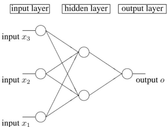
A neural network is a learning system made up of a set of neurons configured in a highly interconnected network. It can learn from examples and exhibit some capability for generalization, beyond the training data. For a feedforward multilayer neural network, the neurons are grouped into three types of layers, namely, input layer, hidden layer and output layer, as shown in Figure 1. Data is fed into the neu-rons in the input layer and then transfer to subsequent lay-ers. At each neuron, weighted inputs arriving from neurons in a preceding layer are computed. A nonlinear function, often called an activation function, is applied to obtain the neuron’s activation value. The activation function is usually a sigmoid function or a hyperbolic tangent function. The function is used to approximate the on-off function. The output value is set to be close to 1 by the function if the sum of the weighted inputs is large. The output is set to a value close to -1 if the sum of the weighted inputs is small. Each neuron has a biasθ which is know as the activation threshold. The weights of connections have been given ini-tial values.

Figure 1. A neural network with three inputs, one output and one hidden layer

k´´ ´´ ¢¢

¢¢ ¢¢

¢¢ k´´

´´ Q

Q Q_Q k

Q Q

Q_Q A

A A

A A

A A

A k´´ ´´ k

Q Q

Q_{Q k} outputo

inputx1 inputx2 inputx3

output layer hidden layer

input layer

There are two types of neural network learning algo-rithms: supervised learning and unsupervised learning. The difference of supervised learning and unsupervised learning is whether or not you have known labels of suggested out-comes during training. Backpropagation [14] is one of the most popular used learning algorithms. It attempts to min-imize the error between the actual (correct) value and the network outputs. The actual outputs are used as supervisors of the training. The error between the output value and the actual value is backpropagated through the network for the updating of the weights.

The architecture of the neural network could be denoted as i-h-o. An i-h-o architecture stands for a neural network

with i neurons in the input layer, h neurons in the hidden layer, and o neurons in the output layer. The neural network in Figure 1 is a 3-2-1 neural network.

The output value for a neuron j is given by the following function:

Oj =G( m

X

i=1

wijxi−θj) (4)

wherexiis the output value of theithneuron in the

previ-ous layer,wij is the weight on the connection from theiij

neuron,θjis the threshold, andmis the number of neurons

in the previous layer. The functionG()is a sigmoid such as a hyperbolic tangent function:

G(z) =tanh(z) =1−e −z

1 +e−z. (5)

In general, a neural network is a function of inputs,X, and weights,w, that isf(X,w). Hornik demonstrated [8] that given a sufficiently complex network, it can provide an accurate approximation to any kind ofX likely to be en-countered. Standard multi-layer feedforward networks are capable of approximating any measurable function to any desired degree of accuracy, in a very specific and satisfying sense. Thus, the “mapping” networks are universal approx-imators. Supervised learning often leads to applications of classification and forecasting in data mining. Unsuper-vised learning may apply to applications where clustering is needed.

4

Sensitivity Analysis

Sensitivity analysis methods estimate the rate of change in the output of a model caused by the changes of the model inputs. It is mainly used to determine which input parame-ter is more important or sensible to achieve accurate output values [15]. It is also used to understand the behavior of the system being modelled, to verify if the model is doing what it is intended to do, to evaluate the applicability of the model, and to determine the stability of a model.

Isukapalli [9] classifies sensitivity analysis methods into the three categories, namely, variation of parameters, domain-wide sensitivity analysis and local sensitivity analy-sis. Variation of parameters or model formulation approach runs a model with different combinations of parameters of concern or with straightforward changes in model structure. Domain-wide sensitivity analysis methods involve the study of the system behavior over the entire range of parameter variation, often taking the uncertainty in the parameter esti-mates into account. Local sensitivity analysis methods fo-cus on estimates of model sensitivity in input and parameter variation in the vicinity of a sample point. This sensitivity is often characterized through gradients or partial derivatives at the sample point.

Frey and Patil [4] classify sensitivity analysis methods into another three categories: mathematical, statistical and graphical. Mathematical methods assess sensitivity in out-put values of models to the range of variation of an inout-put. Statistical methods involve running simulations in which in-puts are assigned probability distributions and then assess-ing the effect of variance in inputs on the output distribution. Statistical methods allow one to identify the effect of inter-actions among multiple inputs. Graphical methods involve information visualization by the representation of sensitiv-ity in the form of graphs, charts, or surfaces. Generally, graphical methods are used to give visual indication of how an output is affected by a variation in inputs.

Sensitivity analysis is normally applied to statistic re-gression models. Similar to rere-gression model

Y=Xβ+ε, (6) whereYis ann×1vector of dependent variables;Xis an n×m(m≤n)matrix of independent variables;βis anm× 1vector of coefficients; andεis ann×1vector of random disturbances, a neural network model can be expressed as

Y=f(X,w), (7) whereX, Yare the same asX, Y in Equation 6 andw is matrix of weights of the neural network. By applying sensitivity analysis, the impact of each independent vari-able on the dependent varivari-ables can also be found. A good and understandable data model can be provided by reduc-ing the number of variables through weight sensitivity anal-ysis [13].

In the case of neural network models, the sensitivity analysis is conducted by analyzing weights of neural net-works. There are three methods, namely equation method, weight magnitude analysis method and variable perturba-tion method, can be used for sensitivity analysis [13]. To simplify the illustration, a feedforward neural network with one hidden layer and one output node is used.

4.1

Equation Method

The first method to be discussed in this section is the equation method [7, 13]. Let wa

bc denote the weight from

the bth _{node in thea}th _{layer to the c}th _{node in the next}

layer. The influence of each input variable on the output can be calculated by the equation:

Ii=

X

k

O(1−O)w2k1vk2(1−v2k)wik1, (8)

where O: the value of the output node; w2

k1: the outgoing weight of thekth node in the second layer; v2

k: the output value of thekthnode

in the second layer; w1

ik: the connection weights between

theith_{node of the first layer and}

thekth_{node in the hidden layer.}

For the equation method, there will benreadings forn input variables for each input row into the network. If there arerinput rows, there will berreadings for each of then input variables. All therreadings for each input variable are subsequently plotted to obtain its mean influence,Ii, on

the output. These values indicate the relative influence each input variable can have on the output variable; the greater the value, the higher the influence. With the ranked ‘Ii’s,

we will know the price of which item is more sensitive to the total profit.

4.2

Weight Magnitude Analysis Method

The second method is the weight magnitude analysis method [13]. The connecting weights between the input and the hidden nodes are observed. The rationale for this method is that variables with higher connecting weights be-tween the input and output nodes will have greater influence on the output node results. For each input node, the sum of its output weight magnitudes to each of the hidden layer nodes is the relative influence of that node on the output. To find the sum of the weight magnitudes from each in-put node, the weight magnitudes of each of the inin-put nodes are first divided by the largest connecting weight magnitude between the input and the hidden layer. This is called nor-malization. The normalization process is a necessary step whereby the weights are adjusted in terms of the largest weight magnitude. The weight magnitudes from each in-put node to the nodes in the hidden layer are subsequently summed and ranked in a descending manner. The rank is an indication of the influence that an input node has on the out-put node relative to the rest. The rank formula is calculated as follows:

Ii=

X

k

w1

ik

maxAll i,k(wik1)

(9) where the notation is the same as in Equation 8. The usage ofIiin the above equation is similar to those in Equation 8.

4.3

Variable Perturbation Method

The third method is the variable perturbation method. This method is more straight forward and different from the previous two. It tests the rate of change in the output with respect to the direct changes of inputs. The previous two methods, namely, equation method and weight magnitude

method analyze indirect changes, i.e., changes of weight in a neural network. We assume that continuous variables are chosen for this analysis. This is because a variable may not be meaningful when it is perturbed. For instance, some nu-meric variable are transferred from nonnunu-meric data. We may use 1, 2, 3 and 4 to represent the four seasons. It does not make sense when we assign the value 1.1 to this vari-able.

This method adjusts the input values of one variable while keeping all the other variables untouched. These changes could take the form of

In⇒In+δ

or

In⇒In×δ,

where I is the input variable to be adjusted and δ is the change introduced toI. The corresponding responses of the output against each change in the input variable are noted. The node whose changes affect the output most is the one considered most influential relative to the rest.

Based on the application and available information, one can select one of the methods introduced in this section. Equation and weight magnitude analysis methods can be used when we know the architecture of the trained neural network models. One can use variable perturbation method when weights and architecture of the neural network model is not available. For instance, when a commercial neural network package is used to build the model. One of the restrictions is that the input variables must be continuous.

5

Sensitivity Analysis for Interesting Mining

Sensitivity analysis of a suitably-trained neural network can determine a set of input variables which have greater influence on the output variable. For example, sensitiv-ity analysis was conducted in order to discover important variables that influence sales performance of color TV sets in the Singapore market with neural networks. It was found that the average price, screen size, flat square, stereo and seasonal factors were most influential on the sale rev-enue [17]. This is consistent with the 4P (Product, Price, Place, and Promotion) marketing mix.

Allocating advertising expenses and forecasting total sales levels are key issues in retailing, especially when many products are covered and significant cross-effects among products are likely. Poh et al. [13] applied sensitiv-ity analysis to a neural network marketing analysis model and found some useful results. These examples show the importance and applicability of sensitivity analysis in dif-ferent domains.

In the case of the scenario described in the introduction section, Equation 3 may be reformulated as,

P=F(MPi, Qi, Ci). (10)

Due to the nonlinearity of the correlation ofMPi,Qi and

Ci, neural networks can be used to model their relationship

with, P, the total profit. Now the elements in Equation 7 are,

Y=P;

X={MP1,· · ·, MPn, Q1,· · ·, Qn, C1,· · ·, Cn}.

In most of the cases,Ci’s are not really independent

vari-ables, i.e., Ci is a function ofMPi andQi. We can thus

simplifyXas{MP1,· · ·, MPn, Q1,· · ·, Qn}since the

re-lationship betweenCi,MPiandQi can be easily captured

by neural networks. We then reformulate Equation 10 as, P =F(MPi, Qi). (11)

One can adopt the following steps to apply interesting mining with sensitivity analysis. First, one may select some independent variables that somehow determine a (set of) dependent variable(s). The total profit in Equation 11 is one example of dependent variables. One may use different types ofPfrom transaction databases to model the relation-ship. For instance,P can be defined as the total profit of a day, a month, a store or even a particular customer. The only requirement is that we must make sure that there is enough data available to build a model.

Second, neural network models are trained in order to find relationships among dependent and independent vari-ables through available data sets. Different input-output combinations, architectures, and activation functions can be tested until a stable neural network model is obtained.

In the third step, one may apply sensitivity analysis to the trained neural network models using one of the three methods described in previous section for the particular ap-plication.

Finally, we may use the knowledge, i.e., the dependent variable is more sensible to a set of independent variables. An action, reducing the retail price for a particular item, for instance, thus can be taken, which should lead to the increase of total sales and profit increase.

6

Conclusion

Although the discovery of interesting and previously un-known patterns are important for data mining applications, it is more important to discover actionable rules. Data min-ing is viewed as the process of turnmin-ing the data into informa-tion, the information into acinforma-tion, and the action into value or profit. The later part of the process attracts much re-search work. This paper shows that sensitivity analysis can

be used for one of the interesting mining tasks, profit min-ing. In particular, we apply neural networks as a general knowledge discovery or data mining tool to model and to discover underlying rules from a data set. Sensitivity anal-ysis is then applied as an optimization procedure to find the most important and sensible factors with respect to profit.

The major difference between the sensitivity analysis proach and other profit mining and interesting mining ap-proaches is that the former approach studies profit mining in a dynamic environment. Further research includes apply-ing sensitivity analysis on different domains, studyapply-ing the differences of three methods discussed in this article, and analyzing the suitability of these methods have on particu-lar applications.

References

[1] Berry, M.J.A., Linoff, G.S., Data Mining Techniques: For Marketing, Sales, and Customer Support, John Wiley & Sons, 1997.

[2] Brijs, T., Goethals, B., Swinnen, G., Vanhoof, K., and Wets, G., “A data mining framework for optimal prod-uct selection in retail supermarket data: the general-ized PROFSET model,” Proceedings of the 6th ACM SIGKDD international conference on Knowledge dis-covery and data mining, 2000, pp300-304.

[3] Embrechts, M. J., Arciniegas, F., Ozdemir, M., Bren-eman, C., Bennett, K. and Lockwood, L., “Bagging neural netwrok sensitivity analysis for feature reduction for insilico drug design”, Proceedings of INNS -IEEE International Joint Conference on Neural Net-works(IJCNN), 2001, pp2478-2482.

[4] Frey, H.C., Patil S., “Identification and review of sensitivity analysis methods”, Proceedings of NCSU/USDA Workshop on Sensititvity Analysis Method, 2001. (Accessed on 15 May, 2003 from http://www.ce.ncsu.edu/risk/pdf/frey.pdf)

[5] Fayyad, U.M., Piatetsky-Shapiro, G. and Smyth, P.,“ From data mining to knowledge discovery: an overview,” in: Advances in knowledge discovery and data mining, Fayyad, U.M., Piatetsky-Shapiro, G., Smyth, P. and Uthurusamy, R. (Eds.), AAAI/MIT Press, 1996, pp1-34.

[6] Han, J., Kamber, M., Data Mining: Concepts and Techniques, Science & Technology Books, 550pp, 2000.

[7] Hashem, S., “Sensitivity analysis for feedforward artificial neural networks with differentiable activa-tion funcactiva-tions”, Proceedings of IJCNN, Vol.1, 1992, pp419-424.

[8] Hornik, K., Stinchcombe, M., and White, H., “Multi-layer feedforward networks are universal approxima-tors”, Neural Networks, 2(5), 1989, 359-366.

[9] Isukapalli, S.S., Uncertainty Analysis of Transport-Transformation Models, PhD Thesis, Rutgers Univer-sity, 1999.

[10] Kleinberg, J., Papadimitriou, C. H. and Raghavan, P., “A microeconomic view of data mining” Data Mining and Knowledge Discovery, 2(4), 311–324, 1998. [11] Lin, T.Y., Yao, Y.Y., and Louie, E., “Mining value

added association rules”, Proceedings of PAKDD, 2002, pp328-333.

[12] Ling, C.X., Chen, T., Yang, Q., and Chen, J., “Min-ing optimal actions for intelligent CRM”, Porceed“Min-ings of IEEE International Conference on Data Mining, 2002, pp767-770.

[13] Poh, H.-L., Yao, J.T. and Jasic, T., “Neural networks for the analysis and forecasting of advertising and promotion impact”, International Journal of Intelli-gent Systems in Accounting, Finance and Manage-ment, 7(4), 253-268, 1998.

[14] Rumelhart, D. E., Hinton, G. E, and Williams, R. J. “Learning internal representations by error propaga-tion”, In D. E. Rumelhart and J. L. McClelland (eds.), Parallel Distributed Processing: Explorations in the Microstructure of Cognition, MIT Press, 1986. [15] Saltelli, A., Chan, K., and Scott, E. M., Sensitivity

Analysis John Wiley & Sons, 2000, pp475.

[16] Wang, K., Zhou, S., and Han, J., “Profit mining: from patterns to actions”, Proceedings of Interna-tional Conference on Extending Database Technology, 2002, pp70-87.

[17] Yao, J.T, Teng, N., Poh, H.-L. and Tan, C.L., “Fore-casting and analysis of marketing data using neural networks”, Journal of Information Science and Engi-neering, 14(4), 523-545, 1998.

[18] Yao, Y.Y., Zhao, Y., and Maguire, R.B., “Explanation-oriented association mining using a combination of unsupervised and supervised learning algorithms,” Proceedings of the Sixteenth Canadian Conference on Artificial Intelligence, 2003.