Available online throug
ISSN 2229 – 5046International Journal of Mathematical Archive- 3 (12), Dec. – 2012 4801
STATISTICAL QUALITY CONTROL OF MULTI-ITEM EOQ MODEL
WITH VARYING LEADING TIME VIA LAGRANGE METHOD
K. A. M. Kotb*, Sayed A. Zaki, Zenab M. Elakkad and S. E. Albendary
Department of Mathematics and Statistics, Faculty of Science, Taif University, Taif, Saudi Arabia.
(Received on: 24-11-12; Revised & Accepted on: 23-12-12)
ABSTRACT
T
he goal of this paper is to confirm that the production process is in control using statistical quality control process with subgroup ranges. The analytical solution of the economic order quantity model of multiple items with varying leading time using Lagrangian multipliers is derived. The varying leading time crashing cost is considered to be continuous function of leading time. The model is restricted to the budget inventory investment. The optimal order quantity is deduced as a decision variable. Finally the model is illustrating by applied example and the average of the subgroup ranges approach is used to confirm that the production process is in control.Keywords: Inventory model, Lagrangian multipliers, economic order quantity (EOQ), multiple items, leading time, statistical quality control, budget inventory investment.
1. INTRODUCTION
Many researchers have considered the single–item economic order quantity inventory models under one or two constraints such as the maximum budget inventory investment, the maximum warehouse space or the average inventory level. They solved these problems either by the classical Lagrangian multipliers method or the method of "equal order interval for each item" as suggested by Page and Paul [15]. They proposed a heuristic approach for allocating n products over m groups. In fact their method is always significantly good except for large number of products as given in Goyal [4, 5, 6]. Shawky and Abou-El-Ata [16] solved a constrained production lot size model with trade policy by Geometric Programming and Lagrangian methods. Other related works were written by Kun-Chan [12], Juneau and Eyler [7], Das and Maiti [2], Mandal and Pal [13], Mehta and Shah [14] and Teng [17].
The problem of inventory models involving lead time as a decision variable have been succinctly described by Ben-Daya and Abdul Raouf [1].
Recently, Kotb and Fergany [9, 10] derived the analytical solution of the economic order quantity model of multiple items with demand-dependent unit cost, leading time and varying holding cost using geometric programming approach.
The statistical quality control for probabilistic and deterministic models is studied by Kotb [8], El-Wakeel [3] and Kotb et al [11].
The aim of this paper is to discuss statistical quality control and inventory policy of deterministic multi-item economic order quantity model with varying leading time under linear constraint which is assumed bending. The optimal order quantity of each item was obtained as decision variable using Lagrangian method. In the final the average of the subgroup ranges approach was used to confirm that the production process is in control.
2. BASIC NOTATIONS AND ASSUMPTIONS
To construct the model of this problem, we define the following variables:
hr
C
= Unit holding (inventory carrying) cost per item per unit time, For the rth item.or
C
= Ordering cost, For the rth item.pr
C
= Unit purchase (production) cost, For the rth item.CL = Control limit.
r
D
= Annual demand rate, For the rth item. K = Limitation of budget inventory investment.r
L
= Leading rate time, For the rth item.Corresponding author: K. A. M. Kotb*
MODEL WITH VARYING LEADING TIME VIA LAGRANGE METHOD /IJMA- 3(12), Dec.-2012.
LCL = Lower control limit.
n = Number of different items carried in inventory.
r
Q
= Production (order) quantity batch (a decision variable), For the rth item. ∗r
Q
= Optimal order quantity, For the rth item.i
R
= Subgroup ranges.R
= Average of subgroup ranges (CL). 2R
S
= Variance of subgroup ranges.SS =
k
σ
L
r = Safety stock, where k is known as safety factor andσ
is standard deviation. TC(
Q
r)
= Average annual total cost. For the rth item.UCL = Upper control limit.
In addition, the following basic assumptions about the model are made: (1) Demand rate
D
r is uniform over time.(2) Time horizon is finite. (3) Shortages are not allowed.
(4) Lead time crashing cost is related to the lead time by a function of the form:
( )
r r,
1, 2 , 3,
,
R L
=
α
L
r
=
n
(1) whereα
>
0
is real constant selected to provide the best fit of the estimated cost function.(5) Our objective is to confirm that the production process is in control.
3. MATHEMATICAL MODEL:
The annual relevant total cost was composed of four components (production, order, inventory carrying and lead time crashing costs) according to the basic notations and assumptions of the EOQ model is:
( )
∑
=
+
+
σ
+
+
=
n 1 r r r r hr r r or r r pr rr
R
L
Q
D
C
L
k
2
Q
C
Q
D
C
D
)
Q
(
TC
(2)To determine the optimal values of
Q
r we Substitute (1) in (2) obtaining:∑
=
α
+
+
σ
+
+
=
n 1 r r r r hr r r or r r pr r rL
Q
D
C
L
k
2
Q
C
Q
D
C
D
)
Q
(
TC
(3)The following constraint can be stated as:
1
,
0
n
pr r r
r
C Q
K
Q
for all r
=
≤
>
∑
(4)where K is the limitation of budget inventory investment.
In order to solve this primal function which was a convex programming problem, it can be rewritten in the following form:
∑
=
α
+
+
σ
+
+
=
n 1 r r r r hr r r or r r pr r rL
Q
D
C
L
k
2
Q
C
Q
D
C
D
)
Q
(
TC
Min
(5)subject to
C
Q
K
n 1 r r pr
≤
∑
=This is a minimization problem in n variables with single constraint. Hence it can be solved by the Lagrangian multiplier approach. The Lagrangian function associated with problem (5) can be restated as:
−
λ
+
α
+
+
σ
+
+
=
λ
∑
∑
= = n 1 r r pr n 1 r r r r hr r r or r r pr r
r
L
K
C
Q
Q
D
C
L
k
2
Q
C
Q
D
C
D
)
,
Q
(
L
(6)© 2012, IJMA. All Rights Reserved 4803
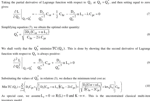
Taking the partial derivative of Lagrange function with respect to
Q
r atQ
r=
Q
*r, and then setting equal to zero, gives:0
C
L
Q
D
C
2
1
C
Q
D
Q
L
pr r 2 * r r hr or 2 * r r Q Q r * r r=
λ
−
α
−
+
−
=
∂
∂
= (7)Simplifying equation (7), we obtain the optimal order quantity:
(
)
pr hr r or r * rC
2
C
L
C
D
2
Q
λ
−
α
+
=
(8)We shall verify that the
Q
*r minimizeTC
(
Q
r)
. This is done by showing that the second derivative of Lagrangefunction with respect to
Q
r is always positive:0
L
Q
D
C
Q
D
Q
L
r 3 * r r or 3 * r r Q Q 2 r 2 * r r>
α
+
=
∂
∂
= (9)Substituting the values of
Q
*r in relation (3), we deduce the minimum total cost as:(
)
(
)
(
(
)
)
∑
= σ + + α + + λ − α + + = n 1 r hr r pr hr r r pr hr r or r pr rr k L C
C 2 C 2 L Cor D C 2 C L C D 2 1 C D ) Q ( TC
Min (10)
As special case, we assume
L
r=
0
⇒
R
(
L
)
=
0
and
K
→
∞
. This is the unconstrained classical multi-item inventory model.4. STATISTICAL QUALITY CONTROL
The decision variables
Q
*r should be computed hose values are to be determined to minimize the total cost and toconfirm that the production process is in control for three items (n = 3). The parameters of the model are shown in TABLE 1:
r
D
rL
rC
orC
prC
hrα
r1 25 Units 8 Weak $ 200 $ 10 $ 0.8 $ 1 2 25 Units 4 Weak $ 140 $ 08 $ 0.5 $ 2
3 25 Units 2 Weak $ 100 $ 05 $ 0.3 $ 3
TABLE 1 Assume that the standard deviation
σ
=
6
units/weak and k = 2.The optimal results of the production batch quantity
Q
*r, the minimum annual total cost and subgroup ranges are givenin TABLE 2 for each values of
λ
:λ
* r
Q
0.00000 - 00900 - 0.00910 - 0.00913 - 0.00914 - 0.00915
* 1
Q
114.0175425 103.0157507 102.9107932 102.8793685 102.868900 102.8584347* 2
Q
121.6552506 107.1946045 107.0616911 107.0219134 107.008664 106.9954195* 3
Q
132.9169136 116.5750556 116.4258872 116.3812482 116.366380 116.3515174Min TC 732.8435354 744.1045510 744.7352781 744.7722876 744.6846213 744.7969535
i
R
018.8984711 013.5593049 013.5150940 013.5018797 013.4974800 013.493080MODEL WITH VARYING LEADING TIME VIA LAGRANGE METHOD /IJMA- 3(12), Dec.-2012.
In order to study the statistical quality control of the model, applying control limit (CL) approach when
σ
is unknown as:The average of the subgroup ranges (CL) is:
41088495
.
14
6
4653097
.
86
6
R
R
6
1 i
i
=
=
=
∑
=
The standard deviation of the subgroup ranges is:
(
)
006985489
.
2
027990753
.
4
6
R
R
S
6
1 i
2 i
R
=
=
−
=
∑
=
The lower control limit is
LCL
=
R
−
3
S
R=
8
.
389928483
, the average of the subgroup ranges is41088495
.
14
R
=
and the upper control limit isUCL
=
R
+
3
S
R=
20
.
43184142
. It is clear thatLCL
<
R
<
UCL
. Therefore the production process is in control.5. CONCLUSION
This paper is devoted to study statistical quality control for multi-item inventory model that considers order quantity as decision variable. An analytical solution of the EOQ model with varying leading time and one restriction is derived using Lagrangian approach. Finally, we used the optimal order quantity of each of the 3 items and subgroup ranges method to investigate quality control of the production process.
REFERENCES
[1] M. Ben-Daya and Abdul Raouf, Inventory Models Involving Lead Time as a Decision Variable, J. Opl. Res. Soc., Vol. 45, No. 5(1994), pp. 579-582.
[2] K. Das and M. Maiti, Inventory of a differential item sold from two shops under single management with shortages and variable demand, Applied Mathematical Modelling, 277(2003), pp. 535-549.
[3] M. F. El-Wakeel, Quality control for probabilistic (Q , r) inventory model with varying order cost and continuous lead time demand under the annual holding constraint, International Journal of Mathematical Archive, 2(7) (2011), 1027-1033.
[4] S. K. Goyal, Optimal ordering policy for a multi-item single supplier system, Operational Research Quarterly, Vol. 25(1975), pp. 293-298.
[5] S. K. Goyal, A note on multi-product inventory situations with one restriction, Journal of the Operational Research Society, Vol. 29, No. 3(1978), pp. 269-271.
[6] S. K. Goyal, Economic order quantity under conditions of permissible delay in payment, Journal of the Operational Research Society, Vol. 36, No. 4(1985), pp. 335-338.
[7] J. Juneau and R. C. Eyler, An economic order quantity model for time-varying demand, The International Journal of Modern Engineering, 1(2001), pp. 1-10.
[8] K. A. M. Kotb, Statistical quality control for constrained multi-item inventory lot-size model with increasing varying holding cost via geometric programming, International Journal of Mathematical Archive, 2(4) (2011), 409-414.
[9] K. A. M. Kotb and H. A. Fergany, Multi-item EOQ model with varying holding cost: A geometric programming approach, Int. Math. Forum, 6(2011), 1135-1144.
[10] K. A. M. Kotb and H. A. Fergany, Multi-item EOQ model with both demand-dependent unit cost and varying leading time via geometric programming, Applied Mathematics, 2(2011), 551-555.
[11] K. A. M. Kotb, H. M. Genedi and S. A. Zaki, Quality control for probabilistic single-item EOQ model with zero lead time under two restrictions: A geometric programming approach, Int. Math. Forum, 6(2011), 1397-1404. [12] Kun-Chan Wu, Deterministic inventory model for items with time varying demand, Weibull distribution
deterioration and shortages, Yugoslav Journal of Operational Research, 12, No. 1(2002), pp. 61-71.
[13] B. Mandal and A. K. Pal, Order level inventory system with ramp type demand rate for deteriorating items, Journal of International Mathematics, 1(1998), pp. 49-66.
[14] N. Mehta and N. Shah, An Inventory model for deteriorating items with exponentially increasing demand and shortages under inflation and time discounting, Investigacao Operational, 23(2003), pp. 103-111.
© 2012, IJMA. All Rights Reserved 4805
[16] Shawky A. I. and M. O. Abou-El-Ata, Constrained production lot-size model with trade credit policy: a comparison geometric programming approach via Lagrange, Production Planning and control, 12(7) (2001), 654-659.
[17] J. T. Teng, A deterministic inventory replenishment model with a linear trend in demand, Operat. Res. Lett. 19(1996), pp. 33-41.