Vol 4, No 2 (2013)

Available online throug

ISSN 2229 – 5046

RAPID PARAMETER ESTIMATION

OF THREE PARAMETER NONLINEAR GROWTH MODELS

1

Prof. Munindra Borah* &

Sri Dimpal Jyoti Mahanta

1

Department of Mathematical Sciences, Tezpur University, Napaam, Tezpur, Assam, PIN 784001

2

Department of mathematical sciences, Tezpur University, Napaam, Tezpur, Assam, PIN 784001

(Received on: 13-12-12; Revised & Accepted on: 05-02-13)

ABSTRACT

T

Keywords: Gompertz model, Logistic model, Monomolecular model, Nonlinear growth model, parameter estimation.

1. INTRODUCTION

Growth is defined as variation and development in tissues and organs of an organism over time. Growth model is one type of simplified representation of a real system, which represents the behaviour of the system. The three parameter non-linear models, Monomolecular, Gompertz and Logistic are commonly used to determine the growth and development of various systems [5, 6]. These models are particular cases of the generalized Chapman-Richards function [8]. Many forestry researchers made extensive and profound studies on these models [3, 8, 13, 14]. In this study, the growth models Monomolecular, Gompertz and Logistic, which are special cases of the generalized Chapman- Richards function for parameter 𝑚𝑚= 0,𝑚𝑚= 1, and 𝑚𝑚= 2 respectively, which are widely used by forestry scholars, have been selected to fit by estimating the parameters using various method of estimations.

Logistic model was developed by Belgian mathematician Pierre Verhulst, who suggested that the rate of population increase may be limited, that is, it may depend on population density. At low densities, the population growth rate is high. Population growth rate declines with population numbers. The dynamics of the population is described by the differential equation:

𝑑𝑑𝑑𝑑 𝑑𝑑𝑑𝑑⁄

𝛼𝛼−𝑑𝑑 =𝑏𝑏0+𝑏𝑏1𝑑𝑑, (1)

where 𝑏𝑏0,𝑏𝑏1 are constant and 𝑑𝑑 and 𝑑𝑑 are the dependent and independent respectively. Which has the following solution

exp{(𝑏𝑏0+𝑏𝑏1𝛼𝛼)𝑑𝑑} =𝛽𝛽(𝑑𝑑+𝑏𝑏0⁄𝑏𝑏1)(𝛼𝛼 − 𝑑𝑑)−1.

If 𝑑𝑑(−∞) = 0, 𝑏𝑏0 must be zero. Hence the logistic growth model is given by

𝑑𝑑(𝑑𝑑) =_{(1+𝛽𝛽exp (}𝛼𝛼 _{−𝑘𝑘𝑑𝑑))}. (2)

where 𝑘𝑘=𝑏𝑏1𝛼𝛼 is related to the rate of increasing of 𝑑𝑑,𝛼𝛼 is the upper asymptote and 𝛽𝛽 is a location parameter[10]. The curve has an S-shape and all the parameters are positive. Also the shape of the curve is symmetric about its point of inflection [1].

Corresponding author:1_{Prof. Munindra Borah*} 1

The mathematical representation of monomolecular growth is borrowed from physical chemistry, where it describes a first order irreversible chemical reaction. In plant nutrition and soil fertility it is also known as the Mitscherlich growth. The monomolecular model has no inflection point and the growth rate decrease linearly as size increasing. Then,

𝑑𝑑𝑑𝑑

𝑑𝑑𝑑𝑑 =𝑘𝑘(𝛼𝛼 − 𝑑𝑑), (3)

where w is the expected size of an organism at time𝑑𝑑, 𝛼𝛼 represents the limiting size of the organism and 𝑘𝑘 is the growth rate parameter [1]. From this differential equation, the required model may be written as

𝑑𝑑(𝑑𝑑) =𝛼𝛼(1− 𝛽𝛽exp(−𝑘𝑘𝑑𝑑)), (4)

where 𝛽𝛽 is the biological constant. This function rises steadily from a point 𝛼𝛼(1− 𝛽𝛽)to the limiting value of 𝛼𝛼.

The Gompertz Model named after Benjamin Gompertz (1779 – 1865). Gompertz model is a sigmoid function. The Gompertz equation arises from models of self-limited growth where the rate decreases exponentially with time. The model was first introduced to describe the growth in the number of tumor cells which usually follows a sigmoidal growth pattern. The model is a solution of the differential equation

𝑑𝑑𝑑𝑑

𝑑𝑑𝑑𝑑 =𝑘𝑘𝑑𝑑 log� 𝛼𝛼

𝑑𝑑�. (5)

By integrating (5), the Gompertz model may be obtained as

𝑑𝑑(𝑑𝑑) =𝛼𝛼exp(−𝛽𝛽exp(−𝑘𝑘𝑑𝑑)), (6)

where 𝑑𝑑is the number of tumor cells at time t, 𝛼𝛼> 0 is the upper limit, 𝛽𝛽> 0 is the biological constant, 𝑘𝑘> 0 is the parameter governing the rate at which the response variable approaches its potential maximum [3,4]. Although this curve is an S-shaped one like the logistic. It is not symmetrical about its point of inflection [1].

Nonlinear models are more difficult to specify and estimate the parameters than linear models. But for prediction purpose it is very important to distinguish these parameters properly. Lots of methods of estimation were developed by various authors[3, 9, 10, 12]. The aim of the paper is to estimate the parameters of the models by using various methods of estimation. By selecting appropriate method of estimation, the best fit model may be obtained based on three sets of well-known forestry data sets. Also the initial (guess) value specification plays a very important role in parameter estimation of nonlinear models using certain iterative methods. The first four methods of this paper will provide the initial value specification for the parameters of Monomolecular, Gompertz and Logistic growth models.

2. MATERIAL AND METHODS

The top height age data originated from the Bowmont Norway spruce thinning experiment, sample plot 3661 [3] has been considered. Top height age data were repeatedly measured on a five year cycle from age 20 to 64 and are presented in Table i. The cumulative basal area production and mean diameter at breast height [2] are also used for testing the validity of the methods.

Table i. Top height growth data from Bowmont Norway spruce thinning experiment, sample plot 3661 [3].

Top height (m) 7.3 9.0 10.9 12.6 13.9 15.4 16.9 18.2 19.0 20 Age (year) 20 25 30 35 40 45 50 55 60 64

The Monomolecular, Gompertz and Logistic nonlinear growth models quantifying the top height age data can be expressed as:

𝑑𝑑𝑖𝑖 =𝑓𝑓(𝑑𝑑𝑖𝑖,𝐁𝐁) +𝜀𝜀𝑖𝑖, (7)

2.1 METHOD OF ESTIMATION

2.1.1 Method A: Estimation based on three equidistant points.

In this method, we use three equidistant points, 𝑑𝑑1,𝑑𝑑2,𝑑𝑑3, from the given data set. Let 𝑛𝑛 be the number of observations,

𝑑𝑑2be the 𝑑𝑑1+𝑛𝑛

2 𝑑𝑑ℎ observation and 𝑑𝑑1 be the observation between the first observation and the (𝑛𝑛 −2)𝑑𝑑ℎ observation so

that the RMSE is least corresponding to that observation.

Let 𝑑𝑑=𝑑𝑑2− 𝑑𝑑1, then 𝑑𝑑3 be the (𝑑𝑑2+𝑑𝑑)𝑑𝑑ℎ observation. Then the required parameter estimates for the Monomolecular growth model are:

𝛼𝛼�=_2𝑑𝑑2𝑑𝑑22_{− 𝑑𝑑1}− 𝑑𝑑1_{− 𝑑𝑑3}𝑑𝑑3 ,

𝛽𝛽̂=(_𝑑𝑑𝑑𝑑2− 𝑑𝑑1)2

22− 𝑑𝑑1𝑑𝑑3�

𝑑𝑑2− 𝑑𝑑1 𝑑𝑑3− 𝑑𝑑2�

𝑑𝑑1 𝑑𝑑 �

,

𝑘𝑘�=1_𝑑𝑑ln�𝑑𝑑2−𝑑𝑑1_𝑑𝑑

3−𝑑𝑑2�, (8)

where 𝑦𝑦_𝑖𝑖 =𝑑𝑑_𝑑𝑑

𝑖𝑖 for 𝑖𝑖= 1, 2 and 3.

The required parameter estimations for the Gompertz growth model are:

𝛼𝛼�= exp�_2𝑦𝑦2𝑦𝑦22_{− 𝑦𝑦}− 𝑦𝑦1𝑦𝑦3 1− 𝑦𝑦3�,

𝛽𝛽̂=− �_𝑦𝑦3(𝑦𝑦₋2₂− 𝑦𝑦_𝑦𝑦21₊)2_𝑦𝑦1�𝑦𝑦_𝑦𝑦32− 𝑦𝑦_{− 𝑦𝑦2}1�

𝑑𝑑1 𝑑𝑑 �

�,

𝑘𝑘�=1_𝑑𝑑ln�𝑦𝑦2−𝑦𝑦1

𝑦𝑦3−𝑦𝑦2�, (9)

where 𝑦𝑦_𝑖𝑖 = ln𝑑𝑑_{𝑑𝑑𝑖𝑖} for 𝑖𝑖= 1, 2 and 3.

The required parameter estimations for the Logistic growth model are:

𝛼𝛼�=2𝑧𝑧_𝑧𝑧2− 𝑧𝑧1− 𝑧𝑧3

22− 𝑧𝑧1𝑧𝑧3 ,

𝛽𝛽̂=

� (𝑧𝑧2−𝑧𝑧1)2

(𝑧𝑧3−2𝑧𝑧2+𝑧𝑧1)� 𝑧𝑧2−𝑧𝑧1 𝑧𝑧3−𝑧𝑧2�

𝑑𝑑1 𝑑𝑑 �

�

� 𝑧𝑧22−𝑧𝑧1𝑧𝑧3

2𝑧𝑧2−𝑧𝑧1−𝑧𝑧3� ,

𝑘𝑘�=1_𝑑𝑑ln�𝑧𝑧2−𝑧𝑧1_𝑧𝑧

3−𝑧𝑧2�, (10)

where 𝑧𝑧_𝑖𝑖 = 1

𝑑𝑑_{𝑑𝑑𝑖𝑖} for 𝑖𝑖= 1, 2 and 3.

2.1.2 Method B: Estimation based on three partial sums.

For Monomolecular growth model, in this method, we divide the range of observations into three equal parts. That is if we consider the number of observations is 𝑛𝑛 then we have to consider𝑚𝑚 such that 𝑚𝑚=𝑛𝑛

3. Now let 𝑆𝑆1be the sum of first 𝑚𝑚 observations, 𝑆𝑆2 be the sum of second 𝑚𝑚 observations and 𝑆𝑆3 be the last 𝑚𝑚 observations. Then the nonlinear parameter estimations for Monomolecular growth model are:

𝛽𝛽̂=𝑚𝑚(𝑆𝑆2− 𝑆𝑆1)3{(𝑆𝑆2− 𝑆𝑆1) 1

𝑚𝑚−(𝑆𝑆₃− 𝑆𝑆₂)𝑚𝑚1}

(𝑆𝑆3− 𝑆𝑆2)𝑚𝑚1(𝑆𝑆₂2− 𝑆𝑆1𝑆𝑆3)(2𝑆𝑆2− 𝑆𝑆3− 𝑆𝑆1)

,

𝑘𝑘�=_𝑚𝑚1log𝑆𝑆2−𝑆𝑆1_𝑆𝑆

3−𝑆𝑆2 . (11)

In this method for Gompertz we have to take the natural logarithm,𝑙𝑙𝑛𝑛, of both sides and then consider as 𝑦𝑦_𝑖𝑖 = ln𝑑𝑑𝑖𝑖;𝑖𝑖= 1,⋯,𝑛𝑛. let 𝐿𝐿1be the sum of first 𝑚𝑚 𝑦𝑦𝑖𝑖s, 𝐿𝐿2 be the sum of second 𝑚𝑚𝑦𝑦𝑖𝑖s and 𝐿𝐿3 be the sum of last 𝑚𝑚𝑦𝑦𝑖𝑖s. Then the nonlinear parameter estimations for the Gompertz model are:

𝛼𝛼�= exp�_𝑚𝑚1 ._𝐿𝐿3𝐿𝐿₋1𝐿𝐿₂3_𝐿𝐿2− 𝐿𝐿₊22_𝐿𝐿1�,

𝛽𝛽̂=_(𝐿𝐿3(₋𝐿𝐿2₂− 𝐿𝐿_𝐿𝐿2+1)3_𝐿𝐿1)2��_𝐿𝐿3𝐿𝐿2− 𝐿𝐿_{− 𝐿𝐿2}1�

1

𝑚𝑚

−1�,

𝑘𝑘�=_𝑚𝑚1ln�𝐿𝐿2−𝐿𝐿1

𝐿𝐿3−𝐿𝐿2�. (12)

Similarly for logistic model, we have to consider 𝑦𝑦_𝑖𝑖 as the reciprocal of 𝑑𝑑_𝑖𝑖; 𝑖𝑖= 1,⋯,𝑛𝑛. let 𝑅𝑅1be the sum of first

𝑚𝑚 𝑦𝑦𝑖𝑖s, 𝑅𝑅2 be the sum of second 𝑚𝑚𝑦𝑦𝑖𝑖s and 𝑅𝑅3 be the sum of last 𝑚𝑚𝑦𝑦𝑖𝑖s. Then the nonlinear parameter estimates for the Logistic model are:

𝛼𝛼�= m/�_𝑅𝑅𝑅𝑅1𝑅𝑅3− 𝑅𝑅22 3−2𝑅𝑅2+𝑅𝑅1�,

𝛽𝛽̂=

(𝑅𝑅2−𝑅𝑅1)3

(𝑅𝑅3−2𝑅𝑅2+𝑅𝑅1)2�1− � 𝑅𝑅2−𝑅𝑅1 𝑅𝑅3−𝑅𝑅2�

1

𝑚𝑚_�

�_𝑚𝑚1. 𝑅𝑅1𝑅𝑅3−𝑅𝑅22 𝑅𝑅3−2𝑅𝑅2+𝑅𝑅1�

,

𝑘𝑘�=_𝑚𝑚1ln�𝐿𝐿2−𝐿𝐿1_𝐿𝐿

3−𝐿𝐿2�. (13)

2.1.3 Method C: Composite method assuming that the parameter k is known from three equidistant points.

The growth models can be linearised as 𝑌𝑌 = 𝐴𝐴 + 𝐵𝐵𝑋𝑋, assuming the parameter k is known. The estimated value of 𝑘𝑘� may be obtained from the method of three equidistance points. Hence, the other parameters𝛼𝛼 and𝛽𝛽 can be estimated using the method of least square [7].

𝐵𝐵�=𝑛𝑛 ∑ 𝑋𝑋𝑌𝑌 −_{𝑛𝑛 ∑ 𝑋𝑋2−}(∑ 𝑋𝑋_{(∑ 𝑋𝑋})(∑ 𝑌𝑌₎₂ ),

𝐴𝐴̂=𝑌𝑌� − 𝐵𝐵�𝑋𝑋�. (14)

where for monomolecular model 𝑌𝑌=𝑑𝑑,𝐴𝐴=𝛼𝛼,𝐵𝐵=−𝛼𝛼𝛽𝛽 and 𝑋𝑋= exp(−𝑘𝑘𝑑𝑑), for Gompertz model 𝑌𝑌= ln𝑑𝑑,

𝐴𝐴= ln𝛼𝛼,𝐵𝐵=−𝛽𝛽 and 𝑋𝑋= exp(−𝑘𝑘𝑑𝑑) and for Logistic model 𝑌𝑌= 1 𝑑𝑑, 𝐴𝐴=

1

𝛼𝛼,𝐵𝐵= 𝛽𝛽

𝛼𝛼 and 𝑋𝑋= exp(−𝑘𝑘𝑑𝑑).

2.1.4 Method D: Composite method assuming that the parameter 𝑘𝑘� is known from method of three partial sums.

The procedure for this method is similar to the earlier one. Here, the estimated value of 𝑘𝑘� may be obtained from the method of three partial sums, instead using the method of three equidistance points.

2.1.5 Method E: Newton-Raphson method under the assumption that the parameter 𝛼𝛼 is known.

For this method, we consider that the parameter 𝛼𝛼 is known. Then to estimate the other two unknown parameters, the sum of residual square Ф has been minimized, where

Ф=∑ �𝑑𝑑𝑛𝑛𝑖𝑖=1 𝑖𝑖− 𝑓𝑓(𝑑𝑑𝑖𝑖,𝐁𝐁)�2, (15)

𝑓𝑓=Ф𝛽𝛽 =∑ ��𝑑𝑑𝑛𝑛𝑖𝑖=1 𝑖𝑖− 𝑓𝑓(𝑑𝑑𝑖𝑖,𝐁𝐁)�� �𝜕𝜕𝑓𝑓_{𝜕𝜕𝛽𝛽}(𝑑𝑑𝑖𝑖,𝐁𝐁)�, (16)

𝑔𝑔=Ф𝑘𝑘=∑ ��𝑑𝑑𝑛𝑛𝑖𝑖=1 𝑖𝑖− 𝑓𝑓(𝑑𝑑𝑖𝑖,𝐁𝐁)�� �𝜕𝜕𝑓𝑓(_{𝜕𝜕𝑘𝑘}𝑑𝑑𝑖𝑖,𝐁𝐁)�. (17)

Now the Newton-Raphson method for two variables [11] may be used to estimate the parameters 𝛽𝛽 and 𝑘𝑘.

For Logistic model, we have to take 𝑙𝑙𝑛𝑛 on both sides. Then the model takes the form

𝑦𝑦=𝑎𝑎+𝑏𝑏exp𝑐𝑐𝑑𝑑, (18)

where 𝑦𝑦=1 𝑑𝑑,𝑎𝑎=

1

𝛼𝛼,𝑏𝑏= 𝛽𝛽

𝛼𝛼 and 𝑐𝑐=−𝑘𝑘. Now it can be written as

𝑦𝑦𝑖𝑖 =𝑓𝑓(𝑑𝑑𝑖𝑖,𝐁𝐁), 𝑖𝑖= 1,2,⋯,𝑛𝑛 (19)

where y is the response variable, 𝑑𝑑 is the independent variable, 𝐁𝐁is the vector of parameters 𝑎𝑎,𝑏𝑏 and 𝑐𝑐. For the Logistic model (18), the parameter 𝑎𝑎 is assumed to be known. Hence the parameter 𝑏𝑏 and 𝑐𝑐 may be estimated in the same way that we have done for the Monomolecular and the Gompertz model.

After getting the value of 𝛽𝛽 and 𝑘𝑘 (𝑏𝑏and 𝑐𝑐, in case of Logistic), the value of 𝛼𝛼 (𝑎𝑎, in case of Logistic) can be estimated as:

Taking the natural logarithm,𝑙𝑙𝑛𝑛, on both side of monomolecular model(4)

ln𝛼𝛼= ln 𝑑𝑑𝑖𝑖

1−𝛽𝛽exp (−𝑘𝑘𝑖𝑖), for 𝑖𝑖= 1,⋯,𝑛𝑛 (20)

Hence 𝛼𝛼� may be estimated as

𝛼𝛼�=� ∏𝑛𝑛𝑖𝑖=1𝑑𝑑𝑖𝑖

∏𝑛𝑛_𝑖𝑖=1(1−𝛽𝛽exp (−𝑘𝑘𝑖𝑖))�

1

𝑛𝑛

. (21)

Taking the natural logarithm, 𝑙𝑙𝑛𝑛, on both side of Gompertz model(6),

ln_𝑑𝑑𝛼𝛼 =𝛽𝛽𝑒𝑒−𝑘𝑘𝑖𝑖_{, for 𝑖𝑖= 1,⋯,𝑛𝑛 . (22)}

Hence 𝛼𝛼� may be estimated as

𝛼𝛼�=�∏ 𝑑𝑑𝑖𝑖�𝑒𝑒𝛽𝛽𝑒𝑒−𝑘𝑘𝑒𝑒

−𝑛𝑛𝑘𝑘₋₁

𝑒𝑒−𝑘𝑘₋₁�

𝑛𝑛

𝑖𝑖=1 �

1_�𝑛𝑛

. (23)

The Logistic model (18) can be written as,

𝑎𝑎=𝑦𝑦𝑖𝑖 − 𝑏𝑏𝑒𝑒𝑐𝑐𝑖𝑖, for𝑖𝑖= 1,⋯,𝑛𝑛 (24)

Hence 𝑎𝑎� may be estimated as

𝑎𝑎�=1_𝑛𝑛(∑𝑛𝑛𝑖𝑖=1𝑦𝑦𝑖𝑖− 𝑏𝑏 ∑𝑛𝑛𝑖𝑖=1𝑒𝑒𝑐𝑐𝑖𝑖). (25)

This process may be repeated using a pre defined stopping criteria.

2.1.6 Method F: Newton- Raphson method under the assumption that the parameter 𝑘𝑘 is known.

Let us take the linear transformation of the Monomolecular model (4) under the assumption that the parameter 𝑘𝑘is known

𝑦𝑦𝑖𝑖 =𝑎𝑎+𝑏𝑏𝑧𝑧𝑖𝑖, where 𝑦𝑦𝑖𝑖 =𝑑𝑑𝑖𝑖, 𝑧𝑧𝑖𝑖 = exp(−𝑖𝑖𝑘𝑘), for 𝑖𝑖= 1,⋯,𝑛𝑛. (26)

Hence 𝛼𝛼�=𝑎𝑎and 𝛽𝛽̂=−𝑏𝑏 𝑎𝑎.

𝑦𝑦𝑖𝑖 =𝑎𝑎+𝑏𝑏𝑧𝑧𝑖𝑖, where 𝑦𝑦𝑖𝑖 =_𝑑𝑑1_𝑖𝑖,𝑧𝑧𝑖𝑖 = exp(−𝑖𝑖𝑘𝑘), for 𝑖𝑖= 1,⋯,𝑛𝑛. (27)

Hence 𝛼𝛼�=1

𝑎𝑎 and 𝛽𝛽̂= 𝑏𝑏 𝑎𝑎.

Hence, the sum of the residual squaresФ for (26) and (27) may be written as

Ф=∑𝑛𝑛𝑖𝑖=1(𝑦𝑦𝑖𝑖− 𝑎𝑎 − 𝑏𝑏𝑧𝑧𝑖𝑖)2, for 𝑖𝑖= 1,⋯,𝑛𝑛 (28)

Now differentiating (28) with respect to 𝑎𝑎and 𝑏𝑏, two normal equations may be obtained as

𝑓𝑓=Ф𝑎𝑎 =∑𝑛𝑛𝑖𝑖=1(𝑦𝑦𝑖𝑖− 𝑎𝑎 − 𝑏𝑏𝑧𝑧𝑖𝑖), (29)

𝑔𝑔=Ф𝑏𝑏=∑𝑛𝑛𝑖𝑖=1{(𝑦𝑦𝑖𝑖𝑧𝑧𝑖𝑖− 𝑎𝑎𝑧𝑧𝑖𝑖− 𝑏𝑏𝑧𝑧𝑖𝑖2}. (30)

Now Newton-Raphson method for two variables may be used to estimate the parameters 𝑎𝑎 and b. After estimating parameters 𝑎𝑎 and 𝑏𝑏 using (29) and (30), the unknown parameter 𝑘𝑘 can also be estimated using

Ф𝑘𝑘 =∑𝑛𝑛𝑖𝑖=1{(𝑦𝑦𝑖𝑖− 𝑎𝑎 − 𝑏𝑏𝑒𝑒𝑏𝑏𝑏𝑏(−𝑘𝑘𝑖𝑖))(𝑖𝑖𝑏𝑏exp(−𝑘𝑘𝑖𝑖)}, (31)

by Newton-Raphson method.

Gompertz model under the assumption that the parameter 𝑘𝑘 is known initially.

The sum of squared residuals may be given as

Ф=∑ �𝑑𝑑𝑛𝑛𝑖𝑖=1 𝑖𝑖− 𝛼𝛼𝑒𝑒−𝛽𝛽𝑧𝑧𝑖𝑖�2, (32)

where 𝑧𝑧_𝑖𝑖 = exp(−𝑖𝑖𝑘𝑘), for 𝑖𝑖= 1,⋯,𝑛𝑛.

Now differentiating (32) and proceeding in like manner to the Monomolecular and Gompertz models, the parameters𝛽𝛽

and 𝛼𝛼 may be obtained.

After estimating the parameters 𝛽𝛽and 𝛼𝛼, the unknown parameter 𝑘𝑘 has to be estimated by minimizing

Ф=∑ �𝑑𝑑𝑖𝑖− 𝛼𝛼𝑒𝑒−𝛽𝛽𝑒𝑒−𝑘𝑘𝑖𝑖�

2

, 𝑛𝑛

𝑖𝑖=1 (33)

Using Newton-Raphson method.

The process may be repeated using a pre-defined stopping criterion.

3. RESULTS

3.1 Initial value specification

The Newton-Raphson method requires an initial value for each parameter be estimated. Initial value specification is one of the most difficult problems encountered in estimating parameters of nonlinear model [1]. If the initial values are too far away from the actual value then the Newton-Raphson method may not converge or we need a large number of iterations [11]. The method A to method D may be useful for estimating the starting values for the parameter estimates. In this paper, the initial values are provided by any one of these four methods of estimation.

3.2 Parameter Estimates and Analysis

Table ii: Monomolecular top height age (𝑚𝑚𝑦𝑦−1) parameter estimates for a Norway spruce stand.

Table iii: Logistic top height age (𝑚𝑚𝑦𝑦−1) parameter estimates for a Norway spruce stand.

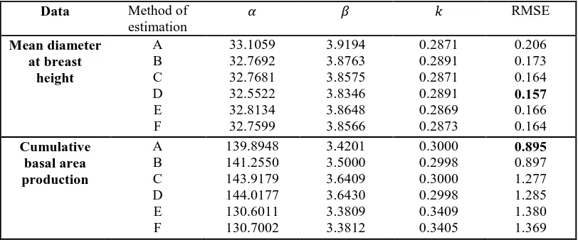
The cumulative basal area production and mean diameter at breast height are also used and the parameter estimates with RMSE value for the Monomolecular, Gompertz and Logistic models are presented in Table v, vi and vii respectively. It is observed that the least RMSE values for Monomolecular and Gompertz growth model for cumulative basal area production are given by method F and which are 0.958m and 0.748m respectively and for the Logistic model is given by method A and which is 0.895m. Again the least RMSE value of Monomolecular, Gompertz and Logistic growth model for mean diameter at breast height are found to be 0.337m, 0.229m and 0.157m with Method F, method F and method D respectively.

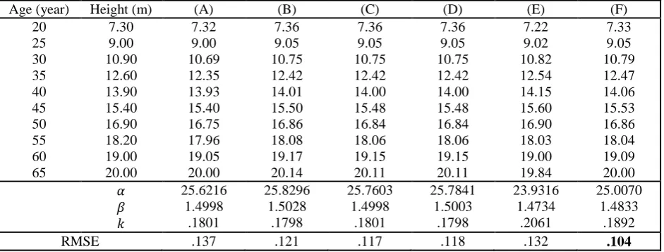
Table iv: Gompertz top height age (𝑚𝑚𝑦𝑦−1) parameter estimates for a Norway spruce stand.

Age (year) Height (m) (A) (B) (C) (D) (E) (F)

20 25 30 35 40 45 50 55 60 65 7.30 9.00 10.90 12.60 13.90 15.40 16.90 18.20 19.00 20.00 7.29 9.16 10.90 12.51 14.01 15.40 16.69 17.89 19.00 20.03 7.26 9.10 10.84 12.47 14.00 15.44 16.79 18.06 19.25 20.38 7.23 9.13 10.89 12.52 14.04 15.45 16.75 17.96 19.09 20.14 7.34 9.15 10.86 12.46 13.97 15.38 16.71 17.96 19.13 20.24 7.23 9.13 10.89 12.52 14.04 15.45 16.76 17.97 19.09 20.13 7.20 9.12 10.90 12.54 14.06 15.46 16.76 17.97 19.08 20.11 𝛼𝛼 𝛽𝛽 𝑘𝑘 33.4000 .8421 .0744 37.8786 .8602 .0621 33.6730 .8458 .0744 37.4481 .8555 .0621 33.5168 .8455 .0750 32.7841 .8436 .0780

RMSE .137 .168 .123 .148 .123 .122

Age (year) Height (m) (A) (B) (C) (D) (E) (F)

20 25 30 35 40 45 50 55 60 65 7.30 9.00 10.90 12.60 13.90 15.40 16.90 18.20 19.00 20.00 7.50 9.00 10.60 12.24 13.86 15.40 16.80 18.05 19.11 20.00 7.41 8.99 10.67 12.38 14.04 15.57 16.93 18.10 19.07 19.85 7.44 8.95 10.58 12.26 13.93 15.52 16.98 18.28 19.40 20.34 7.38 8.97 10.66 12.38 14.06 15.61 17.00 18.19 19.18 19.98 7.34 8.96 10.69 12.43 14.12 15.66 17.02 18.18 19.12 19.88 7.37 8.98 10.69 12.43 14.11 15.66 17.03 18.19 19.15 19.92 𝛼𝛼 𝛽𝛽 𝑘𝑘 23.3317 2.8000 .2822 22.4399 2.7522 .3051 23.8832 2.9319 .2822 22.6302 2.8042 .3051 22.2479 2.7819 .3149 22.3873 2.7811 .3112

RMSE .174 .139 .232 .149 .154 .152

Age (year) Height (m) (A) (B) (C) (D) (E) (F)

20 25 30 35 40 45 50 55 60 65 7.30 9.00 10.90 12.60 13.90 15.40 16.90 18.20 19.00 20.00 7.32 9.00 10.69 12.35 13.93 15.40 16.75 17.96 19.05 20.00 7.36 9.05 10.75 12.42 14.01 15.50 16.86 18.08 19.17 20.14 7.36 9.05 10.75 12.42 14.00 15.48 16.84 18.06 19.15 20.11 7.36 9.05 10.75 12.42 14.00 15.48 16.84 18.06 19.15 20.11 7.22 9.02 10.82 12.54 14.15 15.60 16.90 18.03 19.00 19.84 7.33 9.05 10.79 12.47 14.06 15.53 16.86 18.04 19.09 20.00 𝛼𝛼 𝛽𝛽 𝑘𝑘 25.6216 1.4998 .1801 25.8296 1.5028 .1798 25.7603 1.4998 .1801 25.7841 1.5003 .1798 23.9316 1.4734 .2061 25.0070 1.4833 .1892

Table v: Estimated parameters of Monomolecular model along with RMSE for mean diameter at breast height and cumulative basal area production.

Table vi. Estimated parameters of Gompertz model along with RMSE for mean diameter at breast height and

cumulative basal area production.

Table vii. Estimated parameters of Logistic model along with RMSE for mean diameter at breast height and

cumulative basal area production.

Data Method of

estimation 𝛼𝛼 𝛽𝛽 𝑘𝑘

RMSE

Mean diameter at breast height

A B C D E F 254.2485 197.0727 252.0445 190.6542 106.9216 82.7384 0.9757 0.9708 0.9756 0.9682 0.9460 0.9328 0.0090 0.0123 0.0090 0.0123 0.0238 0.0327 0.415 0.458 0.390 0.378 0.346 0.337 Cumulative basal area production A B C D E F 254.9126 427.8732 252.7398 419.6737 260.2751 246.9026 0.8990 0.9350 0.8988 0.9319 0.9008 0.8973 0.0547 0.0275 0.0547 0.0275 0.0524 0.0566 1.198 1.577 0.961 1.381 0.970 0.958

Data Method of

estimation 𝛼𝛼 𝛽𝛽 𝑘𝑘

RMSE Mean diameter at breast height A B C D E F 42.5918 42.4126 42.3118 41.6907 33.2335 38.0838 1.8758 1.8908 1.8732 1.8628 1.7768 1.8153 0.1445 0.1469 0.1445 0.1469 0.2038 0.1653 0.303 0.320 0.278 0.267 0.361 0.229 Cumulative basal area production A B C D E F 154.2372 175.1747 155.2063 174.9517 147.5676 158.9386 1.6701 1.7565 1.6914 1.7589 1.6857 1.7017 0.1880 0.1589 0.1880 0.1589 0.2055 0.1812 0.867 1.141 0.784 1.115 1.068 0.748

Data Method of

estimation 𝛼𝛼 𝛽𝛽 𝑘𝑘

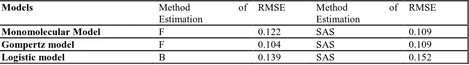
Table viii: RMSE computed using new methods and using SAS for the top height age data.

4. DISCUSSION

The main focus of this paper is to provide some method of estimations required for estimating the parameters of some nonlinear models. The validity of these methods has been tested with some experimental data sets. In estimation of parameters, all the non-linear iterative methods require certain initial value which may be obtained from any one of the first four methods.

It is observed from the above results that the Gompertz model with method F produced the best fit for the top height

age growth data. Method F is defined as the Newton-Raphson method under the assumption that the parameter 𝑘𝑘 is

known. Furthermore the methods presented in the paper produced similar RMSE to those computed using SAS [3], as illustrated in Table viii.

It is observed from the Table ii to Table iv, that the method A; which requires only three equidistant points, the composite method C and iterative method F provide almost same RMSE. If only a few observations are available then the method A and C may be more appropriate.

For cumulative basal area production, the Gompertz growth model with method F provided better RMSE (0.748m) than the other growth models. Again the Monomolecular growth model has the least RMSE for mean diameter at breast height with the method D and which is 0.157m.

Six methods of estimation have been investigated for rapid estimation of parameters of Monomolecular, Logistic and Gompertz models. A comparative study has also been made based on three sets of well-known forestry data. It is noted from our results that method F may be used for estimation of parameters of Monomolecular and Gompertz models, whereas for Logistic model the first four methods may be used.

REFERENCE

[1] Draper, N. R. & Smith, H., Applied regression analysis, John Wiley & Sons Inc, New York, 3rd edition (1998), 706p.

[2] Fekedulegn, D., Theoretical Nonlinear Mathematical Models in Forest Growth And Yield Modelling, Thesis,

Department Of Crop Sciences, Horticulture and Forestry, University College Dublin, Ireland, (1996), 202p.

[3] Fekedulegn, D., Mac Siurtain, M.P. and Colbert, J.J., Parameter estimation of nonlinear growth models in

forestry, Silva Fennica 33(4) (1999), 327–336.

[4] Karkach A. S., Trajectories and models of individual growth, Demographic Research, 15(12) (2006), 347–400.

[5] Kucuk M. and Eyduran E., The Determination of the Best Growth model for Akkaraman and German

Blackheaded mutton x Akkaraman B1crosbreed lambs, Bulgarian Journal of Agricultural Sciences, 15 (1)(2009),

90–92.

[6] Kum D., Karakus K. and Ozdemir T, The best non-linear function for body weight at early phase of norduz

female lambs, Trakia Journal of Sciences, 8(2)(2010), 62-67.

[7] Kapur J. N. and Saxena H. C., Mathematical Statistics, S. Chand and Company Ltd, New Delhi, 20th edition

(Reprint)(2003).362p.

[8] Liu Zhao-gang and Li Feng-ri., The generalized Chapmen- Richards function and applications to tree and stand

growth, Journal of Forestry Research, 14(1) (2003), 19-26.

[9] Mayers, R. H., Montgomery, D. C. and Vining G. G., Generalized linear model with applications in Engineering

and the Sciences, John Wiley & Sons Inc, New York, 1st edition (2002).

[10] Oliver, F. R., Method of estimating the logistic growth function, Applied Statistics 13(1964), 57–66.

[11] Pal Madumangal, Numerical Analysis for Scientists and Engineers: Theory and C Programs, Alpha Science Intl

Ltd, 1stedition (2007).

[12] Shenton, L. R. and Bowman, K. O., Maximum likelihood estimation in small samples, Charles Griffin &

Company ltd, London and High Wycombe, 1st edition (1977).

[13] Vanclay J.K., Modeling Forest Growth and Yield. CAB International, Wallingford, UK, (1994), 312p.

[14] Yuwen S. and Shi L., Growth models and site index table of natural Korean Pine forests, Journal of Forestry

Research, 10(4)(1999), 236-238.

Source of support: Nil, Conflict of interest: None Declared

Models Method of

Estimation

RMSE Method of

Estimation

RMSE

Monomolecular Model F 0.122 SAS 0.109

Gompertz model F 0.104 SAS 0.109