Vol 7, No 3 (2016)

(1)

Available online throug

ISSN 2229 – 5046

GENERAL MANPOWER –SCBZ MACHINE SYSTEM

WITH MARKOVIAN PRODUCTION GENERAL SALES AND GENERAL RECRUITMENT

M. SNEHA LATHA*

Assistant Professor, SRM University, Chennai, Tamil Nadu, India.

(Received On: 17-02-16; Revised & Accepted On: 10-03-16)

ABSTRACT

T

wo Manpower planning models with different recruitment patterns are studied. During the operation time a machine produces random number of products. After the operation time, the sale time starts, which has one among two distinct distributions depending on the magnitude of production is within or exceeding a random threshold. In this paper, the operation times have SCBZ property, production time has exponential distribution and the man power system, operation time, sales and recruitment times have general distributions. Joint transforms of the variables, their means and the covariance of operation time and recruitment time with numerical results are presented

Mathematics Subject Classification: 91B70.

Keywords: Departure and Recruitments, Failure and Repairs, Production and Sale times, Joint transforms.

I. INTRODUCTION

Manpower Planning models have been studied by Grinold and Marshall [2]. For statistical approach one may refer to Bartholomew [1]. Lesson [6] has given methods to compute shortages (Resignations, Dismissals, Deaths). Markovian models are designed for shortage and promotion in MPS by Vassiliou [11]. Subramanian. [10] has made an attempt to provide optimal policy for recruitment, training, promotion and shortages in manpower planning models with special provisions such as time bound promotions, cost of training and voluntary retirement schemes. For other manpower models one may refer Setlhare [9]. For three characteristics system in manpower models one may refer to Mohan and Ramanarayanan [8]. Esary et al. [3] have discussed cumulative damage processes. Stochastic analysis of manpower levels affecting business with varying recruitment rate are presented by Hari Kumar, Sekar and Ramanarayanan [4]. Manpower System with Erlang departure and one by one recruitment is discussed by Hari Kumar [5]. For the study of Semi Markov Models in Manpower planning one may refer Meclean [7].

So far various manpower models have been discussed by many researchers but man power machine system with failure, repair, product production, sales and recruitment have not been together analyzed at any depth. In real life like situation man power is required to run machines which are producing products. Due to employees’ departure and due to machine failure the production system may fail calling for man power recruitment and machine repair. This makes studies on models with production, sales, recruitments and repairs are crucial for any organization and such a study is presented here.

In this paper, a machine which has a varying failure rate property known as switching the clock back to zero (SCBZ) property is considered. The man power system attending the machine is subject failure due to departure of employees. When both are in failed state repairs, recruitments, and sales begin. In this Model, man power vacancies are filled up one by one. The joint Laplace transforms of the operation time of the system, recruitment time, repair time and sale time, their means, covariance of operation and recruitment times are presented with numerical results.

Corresponding Author: M. Sneha Latha*

(2)

1.1 ASSUMPTIONS

1. Inter departure times of employees are independent and identically distributed (i.i.d) random variables with Cdf F(x) and pdf f(x). The manpower collapses with probability p when an employee leaves and with probability q manpower system survives and continues operation where p +q =1.

2. The machine attended by manpower has SCBZ failure property. It has two phases. In phase I it has exponential failure time distribution with parameter ‘a’. If it does not fail in an exponential time with parameter ’c’ it moves to phase 2 and the parameter ‘a’ changes to ‘b’. It has exponential failure time distribution with parameter b.

3. The man power- machine system fails when both are in failed state. When either manpower or machine alone is in failed state, hiring is done to replace the failed unit till the other one also fails and both are in failed state. 4. When the system fails, the vacancies caused by the departure of employees are filled up one by one with

recruitment time V whose Cdf is V(y) and pdf is v(y).

5. When the machine fails (with parameter ‘a’) before the change of parameter, its repair time Cdf is R1(z) and pdf is r1 (z). When it fails after the change of parameter (with parameter b), its repair time Cdf is R2(z) and pdf is r2(z).

6. When the man power-machine system is in operation, products are produced for sales one by one. The inter production times of products have exponential distribution with parameter µ.

7. The sale times of products are i.i.d random variables G with Cdf G(w) and pdf g(w). 8. When the man-power machine system fails, the sale time, recruitment time and repair begin.

1.2 ANALYSIS:

To study the above model the probability density function and the distribution of SCBZ machine life time is required. Since the parameter ‘a’ changes to ‘b’ in an exponential time with parameter ‘c’ if the machine does not fail in phase 1, the life time pdf of machine satisfies the following equation.

( )

0

( )

x

ax cx cu au b x u

h x

=

ae

−

e

−

+

∫

ce

−

e

−

be

− −

du

(1)

The first term of (1) of R.H.S is the pdf part that the machine fails in phase 1 before the change in parameter. The second term is the pdf part that the machine moves to phase2 at time u, no failure occurs in phase 1 and the machine fails at x in phase 2.

On simplification, the pdf of failure time of the machine is

( ) ( )

( )

x a c

cb

(

bx c a x

)

h x

ae

e

c

a b

− + − − +

=

+

−

+ −

(2)

The first term of (2) is phase 1 failure density and the second term of (2) is phase 2 failure density. The survival probability function s(x) of the machine that it does not fail in phase 1 or in phase 2 satisfies the following equation

( ) ( )

0

( )

x

x a c au cu b x u

s x

=

e

− +

+

∫

e

−

ce

−

e

− −

du

(3)

The first term of right side of equation (3) is the probability that the machine survives in phase 1 and second term is the probability that the machine survives in phase 2. On simplification it may be obtained with two probabilities of phase 1 and phase 2 as follows.

( ) ( )

( )

x a c

c

(

b x a c x

)

s x

e

c

a b

− + − − +

=

+

−

+ −

(4)

Simplifying equations (2) and (4), it can be seen as ( )

( )

(

)

x a c bx

h x

=

α

c

+

a e

− +

+

β

be

− (5) and

s x

( )

=

α

e

−x a c( + )

+

β

e

−bx (6)

Here

a b

,

c

and

1 c

a b

c

a b

α

=

−

β

=

α β

+ =

+ −

(7)

(3)

The joint probability density function of four variables, namely

X V R S

, , ,

∧ ∧ ∧













is required for the study of the models Here

(i) X is the manpower-machine system operation time

(ii)

V

∧

the total recruitment time of employees

(iii)

R

∧

is the repair time or the maintenance time of the machine and

(iv)

S

∧

is the total sales time of the products.

When k1 employees have left and k2 products produced then

1 2

....

k 1 2

....

k

V

and S

G

∧ ∧

= +

+

=

+

The repair time

R

∧

is either R1 or R2 according as the machine fails in phase 1 or fails in phase 2. We also note that X is the maximum of the life times of both manpower and machine systems..

We find the pdf f(x, y, z, w) of

X V R S

, , ,

∧ ∧ ∧













as follows.

( ) ( ) 1

1 2

1

( ) ( ) 1

1 2 1 0 0 0

( )

(

) ( )

( )

( , , , )

( )

(

)

( )

(

)

!

x a c bx c a x n

n n

n

x x

u a c b u u a c n

n n n k x k

cb

ae

r z

e

r z

F x pq

v y

c

a b

f x y z w

cb

r z

ae

du

r z

e

du

f x q

pv y

c

a b

x

e

k

µ

∞ − + − − + − = ∞ − + − − + − = ∞ − =





₊

₋







₊







_

_{+ −}



_{ }





_



= 





 





_

₊

₋



 





_

_{+ −}

_

_

_







∑

∫

∑

g w

k

( )













(8)

Here vn(y), fn(x) and gk(w) are n fold convolution of v(y), f(x) and k fold convolution of g(w) with itself respectively. Fn(x) is the n-fold Stiltjes convolution of Cdf F(x) with itself.

To write down the equation (8) the two cases namely (i) the machine fails when the manpower system is in failed state and (ii) the manpower system fails when the machine is in failed state are considered. They are given as two terms inside the flower bracket. The first term has two square brackets. The first square bracket is presented using the terms of equation (2) multiplied by phase 1 and phase 2 failure’s repair densities when the machine fails. The second square bracket is the case of presenting the manpower system already in failed state on the n-th departure and the recruitments for them are done one by one. The second term has two square brackets of which the first one is presented when the machine is already in failed state, the manpower collapses on the n-th departure of an employee. The phase 1 or phase 2 failures, repair densities and the density for n recruitments are presented there to indicate they are done. The last square bracket indicates the k products produced are sold one by one.

We now present the quadruple Laplace transform of the joint pdf of

X V R S

, , ,

∧ ∧ ∧













.

*

0 0 0 0

( , , , )

x y z w

( , , , )

f

ξ η ε δ

e

ξ η ε δ

f x y z w dxdydzdw

∞ ∞ ∞ ∞

− − − −

=

∫∫∫∫

(9)

Because of the structure of equation (8) the equation (9) becomes a single integral as follows. *

( , , , )

f

ξ η ε δ

*

( ) * ( ) *

1 2

* ( )

1

(1 ( )) 1 *

( ) * 1 0 2 1 *

[

( )

(

) ( )]

( )

(1

)

( )

1

1 ( )

[

( )

( )]

n n

x a c bx c a x

x a c

x x g n

n bx c a x

n

n n

cb

ae

r

e

r

c

a b

a

r

e

a

c

e

F x pq

v

cb

e

r

c

a b

b

c

a

f x q

pv

ξ µ δ

(4)

This simplifies as follows

* * * * *

1 2 1 2

1 * * * * 1 2 3 * * 1 2 * * * 2 1 * * 2

1

1 ( , , , )

[

( )

( )]

( )

(

) ( )

1 ( )

( ))

(1

( )

(

))

(

) ( )

(

(1

( )

(

))

cb

a

cb

f

ar

r

c

a b

a

c

a b c

a

pf

v

cb

c

r

q v

f

c

a b

c

a b

pf

v

a

r

qv

f

a

c

ξ η ε δ

ε

χ

η

_ε

η

χ

η

_ε

η

χ





=

_

−

+

_

+ −

+

+ −

+







 

_

_

_

_



+

−



₋

 



_

_{+ −}



_



_

_{+ −}



_





 







+



₋



₊





* * * 3

2 * *

3

(

) ( )

)

( )

(1

( )

(

))

pf

v

c

r

c

a

qv

f

χ

η

ε

η

χ







₊









₊



₋



_



(11) Here * 1 * 2 * 3

(1

( ))

(1

( ))

(1

( ))

g

a

c

g

b and

g

χ ξ µ

δ

χ

ξ µ

δ

χ

ξ µ

δ

= +

−

+ +

= +

−

+

= +

−

(12)

Now the Laplace Transform of the pdf of X is

Now,

* * *

*

* * *

( )

(

)

(

)

( , 0, 0, 0 )

1 ( )

(

) (1

(

))

(

) (1

(

))

pf

a

c

pf

b

f

qf

a

c

qf

a

c

b

qf

b

ξ

αξ

ξ

βξ

ξ

+ +

+

=

−

+ +

−

+ +

+

−

+

(13) Now, *

( )

( , 0, 0, 0 )

0 E X

f

ξ

at

ξ

∂

= −

=

∂

This gives * * * *

( )

(

))

( )

(

) (1

(

))

(1

( ))

E F

pf

a

c

p

f

b

E X

p

a

c

qf

a

c

b

qf

b

α

+

β

=

+

−

+

−

(14)

The Laplace transform of pdf of V is

∧

* *

*

( )

(0, , 0, 0)

1 ( )

pv

f

qv

η

=

−

(15)

*

( )

(0, , 0, 0) |

0 E V

f

η

gives

η

∧

∂

=

∂

( )

E V

p

∧

=

(16)

The Laplace transform of repair time of the machine is

* * *

1 2

(0, 0, , 0)

a

( )

c

( )

f

v

a

c

a

ε

=



_



_

ε

+



_



_

ε

+









₍₁₇₎

*

0

( )

(0, 0, , 0) |

,

E R

f

ε

_ε

gives

ε

∧ =

∂

= −

∂

1 2

( )

a

(

)

c

(

)

E R

a

c

a

c

∧

=

+

₍₁₈₎ The Laplace transform of the sales time is

* * * *

*

* * * *

(1

( ))

(1

( ))

( (1

( ))

(0, 0, 0, )

( (1

( ))

)

( (1

( ))

)

(1

( (1

( ))))

g

pf

g

f

g

a

c

g

b

qf

g

αµ

δ

βµ

δ

µ

δ

µ

δ

µ

δ

µ

δ

−

=

−

+

−

+ +

−

+

−

₍₁₉₎

The expected sales time is

( )

E F

E S

E G

a

c

b

p

α

β

µ

∧





=

_

+ +

_

+

(5)

The joint Laplace transform of Operation time and recruitment time

(

X V

, )

∧

is given by

* * * *

*

* * * *

* *

( )

(

)

( , , 0, 0 )

(1

( )

( ))

(

) (1

( )

(

))

( )

(

)

(

) (1

( )

(

))

pf

v

pv

f

a

c

f

qf

v

a

c

qv

f

a

c

pv

f

b

qv

f

b

ξ

η

αξ

η

ξ

ξ η

ξ

η

ξ

η

ξ

βξ

η

ξ

η

ξ

+ +

=

−

+ +

−

+ +

+

−

+

−

+

₍₂₁₎

The product moment

E X V

(

)

∧

is given by

2 *

(

)

( , , 0, 0 ) |

0 E X V

f

ξ η

∧

_∂

=

= =

∂ ∂

* *

2 * 2 * 2

(1

)

(

)

( )

(

)

( )

(

) (1

(

))

(1

( ))

q

p

f

a

c

p

f

b

E X V

E V

E F

p

a

c

qf

a

c

b

qf

b

α

β

∧



+



=

_

+

_

+

−

+

−





₍₂₂₎

Using the formula

Co v X V

(

)

E X V

(

)

E X E V

(

) ( ),

∧ ∧ ∧

=

−

we can write down the covariance using equations (22), (16) and (14).

II. NUMERICAL EXAMPLES

The usefulness of the results obtained is presented by numerical examples.

Let a =15, b = 5, c =10, p = 0.4, q = 0.6, E (F) =10, E (R1) = 15, E (R2) = 10, E(G) = 12, E(V) = 10, μ = 5, 10, 15, 20, 25 and δ = 2, 4, 6, 8, 10

Here ‘f’ is an exponential density function with parameter ‘δ’.

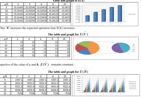
Table and graph of E(X)

μ/δ 2 4 6 8 10

5 25.01441 25.02545 25.03418 25.04129 25.0472

10 25.01441 25.02545 25.03418 25.04129 25.0472

15 25.01441 25.02545 25.03418 25.04129 25.0472

20 25.01441 25.02545 25.03418 25.04129 25.0472

25 25.01441 25.02545 25.03418 25.04129 25.0472

When ‘𝛅𝛅’ increases the expected operation time E(X) increases.

The table and graph for

E V

( )

∧

μ/δ 2 4 6 8 10

5 13 13 13 13 13

10 13 13 13 13 13

15 13 13 13 13 13

20 13 13 13 13 13

25 13 13 13 13 13

Irrespective of the value of μ and 𝛅𝛅,

E V

( )

∧

remains constant.

E R

( )

∧

μ/δ 2 4 6 8 10

5 1507.2 1507.2 1507.2 1507.2 1507.2

10 3014.4 3014.4 3014.4 3014.4 3014.4

15 4521.6 4521.6 4521.6 4521.6 4521.6

20 6028.8 6028.8 6028.8 6028.8 6028.8

25 7536 7536 7536 7536 7536

When μ increases the expected repair time

E R

( )

∧

(6)

E S

( )

∧

μ/δ 2 4 6 8 10

5 25 25 25 25 25

10 25 25 25 25 25

15 25 25 25 25 25

20 25 25 25 25 25

25 25 25 25 25 25

Irrespective of the value of μ and 𝛅𝛅,

E S

( )

∧

remains constant.

E X V

(

)

∧

μ/δ 2 4 6 8 10

5 1000.173 1000.344 1000.502 1000.645 1000.774 10 1000.173 1000.344 1000.502 1000.645 1000.774 15 1000.173 1000.344 1000.502 1000.645 1000.774 20 1000.173 1000.344 1000.502 1000.645 1000.774 25 1000.173 1000.344 1000.502 1000.645 1000.774

When 𝛅𝛅 increases

E X V

(

)

∧

increases.

Cov X V

(

)

∧

μ/δ 2 4 6 8 10

5 374.8126 374.7076 374.6473 374.6129 374.594 10 374.8126 374.7076 374.6473 374.6129 374.594 15 374.8126 374.7076 374.6473 374.6129 374.594 20 374.8126 374.7076 374.6473 374.6129 374.594 25 374.8126 374.7076 374.6473 374.6129 374.594

When 𝛅𝛅 increases

Cov X V

(

)

∧

decreases

REFERENCES

1. Barthlomew.D.J, Statistical technique for manpower planning, John Wiley, Chichester(1979).

2. Esary.J.D, A.W. Marshall, F. Proschan, Shock models and wear processes, Ann. Probability, 1, No. 4 (1973), 627-649.

3. Grinold.R.C, Marshall.K.T, Manpower Planning models, North Holl, Newyork (1977).

4. Hari Kumar.K, P.Sekar and R.Ramanarayanan, Stochastic Analysis of Manpower levels affecting business with varying Recruitment rate, International Journal of Applied Mathematics, Vol.8,2014 no.29, 1421-1428. 5. Hari Kumar.K, Manpower System with Erlang departure and one by one Recruitment, International Journal of

Mathematical Archive-5(7), 2014, 89-92.ISSN 2229-5046.

6. Lesson .G.W, Wastage and Promotion in desired Manpower Structures, J.Opl.Res.Soc. 33(1982)433-442. 7. McClean, Semi-Markovian Models in continuous time, J. Appl. Prob., 16(1980), 416-422.

8. Mohan.C and Ramanarayanan.R, An analysis of Manpower, Money and Business with Random Environments, International Journal of Applied Mathematics, 23(5) (2010), 927-940.

9. Setlhare, Modeling of an intermittenly busy manpower system, In Proceedings at the Conference held in sept,2006 at Gabarone, Botswana(2007).

10. Subramanian.V, Optimum promotion rate in manpower models. International Journal of Management and system,12(2) (1996),179-184.

11. Vassiliou.P.C.G, A higher order Markovian model for prediction of wastage in manpower system, Operat, Res.Quart., 27 (1976).

Source of support: Nil, Conflict of interest: None Declared