Volume 32: Graph-Based Tools 2010

(1)

Proceedings of the

Fourth International Workshop on

Graph-Based Tools

(GraBaTs 2010)

Visualization of Traceability Models

with Domain-specific Layouting

´

Abel Hegedüs, Zoltán Ujhelyi, István Ráth and Ákos Horváth

14 pages

Guest Editors: Juan de Lara, Daniel Varro

Managing Editors: Tiziana Margaria, Julia Padberg, Gabriele Taentzer

(2)

Visualization of Traceability Models

with Domain-specific Layouting

´

Abel Heged üs, Zoltán Ujhelyi, István Ráth and Ákos Horváth∗

(hegedusa,ujhelyiz,rath,ahorvath)@mit.bme.hu,http://www.inf.mit.bme.hu/en Department of Measurement and Information Systems (MIT)

Budapest University of Technology and Economics (BME), Budapest, Hungary

Abstract:Traceability models are often used to describe the correspondence between source and target models of model transformations. Although the visual representa-tion of such models are important for transformarepresenta-tion development and applicarepresenta-tion, mostly ad-hoc solutions are present in industrial environments. In this paper we present a user interface component for visualizing traceability models inside trans-formation frameworks. As generic graph visualization methods fail to emphasize the underlying logical structure of our model, we used domain-specific layouts by customizing generic graph layout algorithms with data from the metamodels used during the transformation. This approach was evaluated, among others, with the traceability models generated by a BPEL verification transformation, which serves as our running example.

Keywords:traceability, graph visualization, domain-specific layout algorithms

1 Introduction

Model transformations are applied increasingly in various fields of software engineering, from business process modeling to formal verification to code generation. The models acting as source and target for the transformations often represent different domains, thus the identification of correspondence between them is non-trivial. Although in the field of critical systems and

services the precise recording oftraceability informationis a strict requirement, in many industrial

applications only ad-hoc solutions are used for handling this information.

Throughout the lifecycle of a system or product, traceability information is generated and used for various tasks. The correspondence information is most often created at the time when the target model is produced using the source model during the execution of the transformation. This information can be later used for validation, verification, change management, maintenance or back-annotation. Traceability information itself can be accessed with model transformations thus

model-based traceability solutionsare advantageous [DKPF09].

A development environment that supports both the generation and visualization of traceability

information can enhance bothautomatic verificationandhuman reviews during certification. We

argue that instead of viewing this information textually or as structured data, it should be stored astraceability models and visualized graphically. After examining the most commongeneric

∗_{This work was partially supported by the SecureChange (ICT-FET-231101) and the C}_ERTI_M_O_{T (ERC HU 09)}

(3)

graph visualizationmethods with traceability models, we concluded that they fail to emphasize the underlying logical structure and mental map, thus a different approach is required.

In this paper we present adomain-specific visualizationmethod for traceability models by

customizing generic layout algorithms. Our approach results in a comprehensive visualization better suited for model transformation debugging purposes than existing approaches. We also outline the general techniques used for constructing domain-specific layouts for traceability models, and discuss various usage scenarios of the visualization during the transformation development process.

Our concepts are presented on a complex running example (implemented during the SENSO

-RIAEuropean project [SEN05]) that aims at providing automated support for the verification of

processes defined in the Business Process Execution Language (BPEL) [OAS07]. The example

includes a complex model transformation, which generates a formal transition system description from the selected BPEL process together with a traceability model, which stores the correspon-dence information between the source and target models. Apart from transformation development, the traceability model is used for aiding the verification and for supporting back-annotation by projecting the verification results from the transition system level to the business process level.

The rest of the paper is structured as follows. Section 2summarizes our running example

for the model checking of BPEL business processes using the Symbolic Analysis Laboratory

(SAL) [Sha00] model checking framework. Section 3 presents the traceability aspects of the

example and the traceability model, including its generation and use. Then,Section 4presents

how generic and domain-specific layout algorithms can be used to visualize traceability models,

and demonstrates them using an implementation in the VIATRA2 framework [V2]. Section 5

assesses the related work and finally,Section 6concludes our paper by evaluating the presented

method and suggesting possible future research directions.

2 Case study: Formal Verification of BPEL Processes

Business processes implemented in BPEL are often used to create business-to-business collabora-tions and complex web services. Their quality is critical to the organization and any malfunction may have a significant negative impact on financial aspects. To minimize the possibility of failures, designers and analysts need powerful tools to guarantee the correctness of business workflows. As the running example of our paper we use such a tool (BPEL2SAL) implemented based on the

method presented in [GHV10].

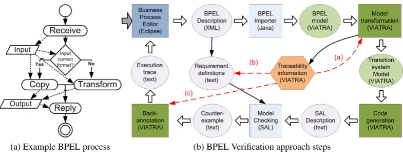
In order to verify BPEL processes, first the input process description istransformed into a

formal model (i.e. state transition systems, see Figure1b), thus defining precise formal semantics

for BPEL. In the second stage, this transition system is projected into the language of SAL bycode

generationexecuted using the VIATRA2 framework. The actual verification is then carried out by

(4)

manually for process-specific requirements), while model checking results in a counter-example

(sequence of transitions) if the requirement is violated by the model. Finally, theback-annotation

of the verification results is provided by another transformation using the traceability information

generated during the first transformation [HBRV10].

(a) Example BPEL process (b) BPEL Verification approach steps

Figure 1: Running Example

Example business processThe input of the tool is a BPEL process therefore, for illustration

purposes, we will use the process shown in Figure1a. The process represents a simple web

service responsible for checking the data format of the input and transforming it if required. TheReceiveactivity stores the incoming message from the requester in theinputvariable,

then the format check decides whether the data is well-formed. If it is valid, theCopyactivity

copies the data into theoutputvariable, otherwise theTransformactivity executes some

manipulation before writing the result into theoutputvariable. Finally theReplyactivity

sends the data from theoutputvariable to the requester and the process finishes.

It is important to note, that business processes are usually larger than our example, however given that BPEL is an executable language, complex processes are implemented in BPEL by orchestration and cooperation of smaller processes (using web-service invocations) instead of in one large BPEL process.

Traceability aspects In the BPEL2SAL tool all steps including model generation, model checkingandback-annotationrequire adequate traceability information concerning the relation

between the source (BPEL) and target (SAL) models (see the dashed arrows in Figure1b: (a)

tosimplify the model transformationby providing pointers to target model elements in different

phases of the structural transformation (b) in order tocapture the requirementsproperly in LTL

expressions where SAL variables have to be used instead of BPEL elements, (c) in back-annotation toderive the BPEL process executionfrom the SAL counter-example. Furthermore, during the development of the transformations it was used for debugging purposes.

Throughout the paper, we will use this traceability information as a domain-specific model for which a graph layout is defined using the presented algorithm. Although presented in the context of the BPEL2SAL tool, these aspects (a-c) can be identified in many other transformation problems

as general concerns [GLMD09]. The traceability information is (i) reused in the transformation,

(5)

3 Static Traceability Models

The collected traceability information, which stores the correspondence between the structure of

models, is called astatic traceability model. Such models are used for various purposes, some of

which are presented through our running example.

Traceability MetamodelIn order to store traceability information a third model called the

traceability modelis created during transformation execution (the BPEL, SAL and traceability

models are stored separately). The traceability metamodel (illustrated on Figure2) used in the

BPEL2SAL approach has similarities to those presented e.g. in [R ¨OV09,DKPF09].

Figure 2: Traceability metamodel The core of the traceability metamodel is

thetraceability record(TR), which represents a correspondence relation between source and target model elements. The record stores rela-tions, which either point to source model

ele-ments (ref sourcerelation) or target model

elements (ref targetrelation). Note that

this basic metamodel allows multiple relations

between source, traceability and target model elements (e.g. a source element can connect to several TRs and TRs may have multiple corresponding source or target elements).

Although the TR could be used directly for creating traceability model instances the definition ofsubtypes(e.g.Receive2Identifier) provides a better solution for using the traceability model (e.g. by simplifying pattern matching).

Note that while we use the simple traceability metamodel defined above throughout the paper as an example, the approach itself does not depend explicitly on this specific metamodel. The only characteristic exploited is the ability to classify relations based on which model elements (source or target) they connect to. Therefore our approach is usable with arbitrary traceability metamodels featuring this characteristic.

Traceability Use Cases: Reuse, Identification and Back-annotation The importance of

traceability can be illustrated on the running example (see Figure 1b) by pointing out three

scenarios in which the traceability model supports the execution of the different steps of the

BPEL2SAL method: (a)reuse, (b)identificationand (c)back-annotation. These steps are found

in many transformation use cases, while visualization is highly convenient for these scenarios as an assistance tool for transformation development and verification.

(a) ReuseThe SAL transition system has separate parts, which are generated at different phases of the transformation. Thus the traceability model is used repeatedly to find the corresponding variables to the relevant BPEL elements (e.g. find the SAL element corresponding to the BPEL

variableinput, which is written during the execution of the Receiveactivity). Note that

generally transformations can be separated to phases thus this scenario appears in many cases

(e.g. in Triple Graph Grammars [Sch95] the correspondence structure can be present in the

precondition of rules).

(b) IdentificationThe requirements, which arevalidated against the business process, can be

best described using the source model (i.e. the BPEL process itself [XLW08]). However they have

(6)

transition system variables). The traceability model can be used to identify corresponding SAL and

BPEL elements (e.g. SAL variable to describe thatReceivealways finishes). Although general

requirements can be defined automatically, domain-specific requirements have to be created manually where visualization of the traceability model can be considered a big improvement compared to other approaches.

(c) Back-annotationThe result of the model checking is a counter-example if the requirement

is violated by asequence of transitionsfrom the initial state leading to a violating state. However

the interpretation (or back-annotation) in the original BPEL process is far from trivial [HBRV10].

The traceability model is used tofind corresponding source elementsfor the SAL variables in

order to derive the BPEL execution from the steps of the counter-example (e.g. the assignment

stating that the SAL variable corresponding to theReceiveactivity changed its value after a

given transition execution). Ideally, back-annotation itself may be automated, the visualization of traceability models is still advantageous during its development.

4 Visualization of Traceability Models

Displaying generated traceability models gives an overview of the status of model transformation, as ideally for every created target model element there should be one or more element in the source model referenced by traceability records. However, not all the source model elements have traceability records, therefore the visualization displays only nodes with records, as the subset with traceability records is usually the significant part.

As the connections are their central element, traceability models can be meaningfully visualized as a graph with the model elements as nodes and the traceability relations as arcs between them. In this section our main contribution is to describe a domain-specific graph layout algorithm created from generic and parameterizable algorithms to visualize such traceability models.

4.1 Visualization of Static Traceability Models

We examined various generic layout algorithms [KW01] to visualize static traceability models.

These algorithms evaluate aesthetic conditions to determine the layout of the graph, without any specific information about the logical structure of the underlying model.

The simplegrid layoutdisplayed nodes in rows and columns, but without additional information

the node positions had no connection with the structure, and the arcs were crossing both nodes

and each other, similar to layout inFigure 4a.

Theradial layout, developed for the drawing of trees by positioning the nodes in concentric circles, displayed the traceability model in two concentric circles: in the middle the traceability records were displayed, while the outer circle contained both the source and target model elements, mixed together. Although the traceability records are clearly identifiable, the created graph does not reflect the structure of the model very well.

(7)

Visualization RequirementsThe empirical evaluation of the generic graph layout algorithms lead us to identifying the following requirements for a graph layout algorithm to visualize static traceability models:

R1. The displayed nodes should not overlap, as it makes identification of nodes difficult.

R2. The crossings of the displayed arcs should be minimized, as this simple aesthetic criteria is

shown to affect human understanding greatly [Pur97].

R3. The corresponding source, target and traceability model elements should be placed close to each other for emphasizing the relations between the model elements. By putting the related

elements close, requirementR2becomes easier to fulfill, as it reduces the arc lengths.

R4. The visualization should clearly separate the source, target and traceability models. As the distinction of the three models forms the basis of the underlying structure, we consider this requirement critical for an understandable visualization.

R5. In order to provide a meaningful visualization during the transformation execution, it is important to handle changes of the input models. The layout should change fast enough,

and should keep unchanged parts similar (as in the mental map maintaining [ELMS91]).

Grid Radial Spring R1

R2 R3 R4 R5

Yes Partial Partial No Yes No No Partial Yes No No No No Yes Partial

Figure 3: Layouts and Requirements

All listed generic layouts clearly violate the R4 requirement. In

addition to that the grid and spring layouts violate theR2crossing

re-quirement, the radial layout theR3closeness requirement (as traceability

records get far from the connected source and target elements).

RequirementsR1,R2andR3are simple aesthetic properties of the

created graph visualization, so they can be fulfilled using generic graph layout algorithms.

On the other hand, as the source and target models are symmetrically connected to the traceability record (as seen in the traceability

meta-model inFigure 2), theR4separation requirement cannot be fulfilled without some

(meta)model-specific information. This information can be presented in the form of a categorization function, that tells for every model element (or model element type) which model it belongs to.

For this reason we propose a domain-specific layout algorithm, that is created by adding model-dependent customizations to existing generic layout algorithms.

4.2 Domain-specific Layout Algorithm for Static Traceability Models

In this paper we propose the use of domain-specific layouting by customizing generic and parameterized algorithms: we give extra information based on the source, traceability and target metamodels. The customization takes the following steps: (1) filtering the model, (2) creating a custom ordering of the model elements and (3) adjusting the layout algorithm to satisfy further visual constraints.

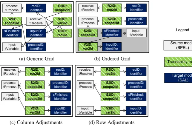
The different problems we addressed with the use of domain-specific layout algorithms for

traceability visualization are illustrated inFigure 4. In each figure we use a small subset of the

(8)

r_s r_t receive: tReceive R2ID: rec2id recID: identifier process: tProcess S2ID: scope2id processID: identifier S2ID: scope2id sFinished: identifier receive: tReceive R2ID: rec2id recID: identifier process: tProcess S2ID: scope2id processID: identifier S2ID: scope2id receive: tReceive R2ID: rec2id recID: identifier process: tProcess S2ID: scope2id processID: identifier S2ID: scope2id sFinished: identifier input: tVariable V2ID: var2id inputID: identifier input: tVariable V2ID: var2id input: tVariable V2ID: var2id inputID: identifier sFinished: identifier inputID: identifier receive: tReceive R2ID: rec2id recID: identifier process: tProcess S2ID: scope2id processID: identifier S2ID: scope2id sFinished: identifier input: tVariable V2ID: var2id inputID: identifier Source model (BPEL) Target model (SAL) Traceability model Legend

(a) Generic Grid

(b) Ordered Grid

r_s r_t receive: tReceive R2ID: rec2id recID: identifier process:

tProcess scope2idS2ID:

processID: identifier S2ID: scope2id sFinished: identifier receive: tReceive R2ID: rec2id recID: identifier process:

processID: identifier S2ID: scope2id receive: tReceive R2ID: rec2id recID: identifier process: tProcess S2ID: scope2id processID: identifier S2ID: scope2id sFinished: identifier input: tVariable V2ID: var2id inputID: identifier input: tVariable V2ID: var2id input: tVariable V2ID: var2id inputID: identifier sFinished: identifier inputID: identifier receive: tReceive R2ID: rec2id recID: identifier process:

processID: identifier S2ID: scope2id sFinished: identifier input: tVariable V2ID: var2id inputID: identifier Source model (BPEL) Target model (SAL) Traceability model Legend r_s r_t receive: tReceive R2ID: rec2id recID: identifier process: tProcess S2ID: scope2id processID: identifier S2ID: scope2id sFinished: identifier receive: tReceive R2ID: rec2id recID: identifier process: tProcess S2ID: scope2id processID: identifier S2ID: scope2id receive: tReceive R2ID: rec2id recID: identifier process: tProcess S2ID: scope2id processID: identifier S2ID: scope2id sFinished: identifier input: tVariable V2ID: var2id inputID: identifier input: tVariable V2ID: var2id input: tVariable V2ID: var2id inputID: identifier sFinished: identifier inputID: identifier receive: tReceive R2ID: rec2id recID: identifier process: tProcess S2ID: scope2id processID: identifier S2ID: scope2id sFinished: identifier input: tVariable V2ID: var2id inputID: identifier Source model (BPEL) Target model (SAL) Traceability model Legend

(c) Column Adjustments

(d) Row Adjustments

r_s r_t receive: tReceive R2ID: rec2id recID: identifier process:

processID: identifier S2ID: scope2id sFinished: identifier receive: tReceive R2ID: rec2id recID: identifier process:

processID: identifier S2ID: scope2id receive: tReceive R2ID: rec2id recID: identifier process: tProcess S2ID: scope2id processID: identifier S2ID: scope2id sFinished: identifier input: tVariable V2ID: var2id inputID: identifier input: tVariable V2ID: var2id input: tVariable V2ID: var2id inputID: identifier sFinished: identifier inputID: identifier receive: tReceive R2ID: rec2id recID: identifier process:

processID: identifier S2ID: scope2id sFinished: identifier input: tVariable V2ID: var2id inputID: identifier Source model (BPEL) Target model (SAL) Traceability model Legend

Figure 4: Visualizing the Traceability Model

their corresponding identifiers from the SAL model (SAL variables) and the traceability records in-between. The different parts of the graph are colored differently, and the arc captions are removed to maintain readability of the graphs.

Algorithm selectionWe have chosen a three-column grid layout algorithm, as columns could

provide a clean separation of the different parts (thus fulfilling requirementR4). Although the

generic grid layout gives the worst visualization results without further information, it is easier to customize using incorporated domain-specific information.

The generic grid layout does not distinguish between different parts of the model, instead it

places the nodes in an unpredictable way similar to the layout inFigure 4a. It is important to note,

that the generic layout algorithm does not utilize domain-specific filtering, however for the sake of readability we omitted some (from the traceability point of view) less relevant elements from the figures, like the internal structure of the source or target models.

FilteringThe use of (meta)model-dependent filters helps to provide more relevant domain-specific layout algorithm: by removing unnecessary entities or relations the resulting visualization becomes more focused.

When displaying the traceability model, the intra-model relations of source or target models are often unimportant. By filtering out these relations the resulting visualization is more relevant.

Removing irrelevant nodes or relations also reduces the number of crossing arcs (requirementR2).

The removed intra-model relations can either be evaluated using the existing model space editors or a less strict filter should be applied. When applying such a filter, in order to keep the visualization readable, the source, target and traceability models should be filtered similarly. The development of such filters are planned in the future.

In case of huge models a large number of nodes/connections may remain visible after the filter

application (e.g. about 300 nodes are displayed in the SENSORIAcase study [AD07]), emphasizing

(9)

Filters can also be defined in the user interface: the user can decide which elements are relevant, and others can be filtered out. This can be used as a kind of search functionality inside the traceability model: it is possible to list only a type from the source or target model, and display its corresponding nodes.

The filtering can happen on both the model and metamodel level: in the first case it is possible to filter out some model elements (typically initiated by the user on the user interface), or entire types (typically built-in filters, provided by the framework).

OrderingCustom ordering can be used to force an algorithm to place the nodes in a predefined order. It is important to note, that some layout algorithms, such as the grid layout are dependent on the ordering of nodes, but others, typically force-based algorithms (e.g. radial, spring) are ordering-insensitive.

The grid layout implementation used for traceability visualization places the nodes in the order it receives them. Therefore by creating an ordering that puts the corresponding nodes next to each other in source-traceability-target order, the layout will place them next to each other. Secondary ordering can be used to order the tuples by their relations.

Our solution ordered the items by the name of the traceability records (source and target models are ordered by the names of their corresponding traceability nodes). The ordering ensures that corresponding elements are placed close to each other, and can often be connected without arc

crossings (requirementR3andR2respectively).

This simple ordering works very well if there is one-to-one correspondence between the different source, traceability and target model elements, otherwise elements get misplaced between

columns. As bothS2IDelements in the grayed area ofFigure 4b are connected to the same

processnode, they should be placed into the second column, but the ordering misplaced them.

Further Visualization ConstraintsDomain-specific knowledge (e.g. the type of the nodes) makes the layout algorithm capable of more efficient visualization. Filtering and ordering cannot utilize all this information, so slight alterations of the layout algorithm might be needed.

For our traceability visualization the grid layout has been altered in two ways: (1) the algo-rithm decides which model the model elements belong to (simple categorization based on the

metamodel), and places it into its corresponding column (requirementR4), and (2) grid cells are

left empty to align the corresponding model elements together (requirementR3). The second

adjustment is needed, as the first one only ensures that every element appears in the intended

column, but an element can get into a wrong row (as theinputelement inFigure 4c). This issue

is addressed by ensuring that for every source, traceability and target tuple a new row is started in

the layout (seeFigure 4d).

(10)

model manipulations by the BPEL2SAL transformation, while a change in the source (BPEL) model requires the re-execution of the transformation.

The deletion of elements often results in the deletion of a row, also causing row shifting. If instead of deleting the elements they would be marked dirty (i.e. a signal representing the deletion), the layout could be altered to leave their places empty.

We consider that even the basic version of our approach fulfills the change handling

require-mentR5, as typically complete rows are shifted, so locally the mental map is maintained. By

applying the mentioned optimizations the changes can be emphasized.

4.3 Evaluation of the Approach

The visualization fulfills all requirements (R1–R5), and emphasizes the logical structure of the

transformation: the three models are clearly separated in columns, while the connected elements are grouped in rows. A big drawback of our layout algorithm is the large space consumption, especially vertically. This means, vertical scrolling is almost always needed, but that is easy to understand, and does not affect the usability of our solution. It is also possible to enhance the usability of the solution by more advanced filtering options (thus increasing readability), or some kind of searching option (to make the model navigable).

The created visualization can handle large models, we used the SENSORIA Finance case

study [AD07] for evaluation, whose BPEL, traceability and SAL models contain 220,116,6647

elements, respectively. After applying the filters, the remaining elements are visualized resulting in a graph about 300 nodes large. The visualization is initialized in less than a second, and could

be updated fast enough (approx. 50ms) to be usable in a changing environment as well.

Although our approach was only tested using traceability models, where a single traceability record is connected to one source and one target element, we believe, the resulting visualization could also be used with more complex traceability records with more source and/or target elements. In this case it is possible, that arc crossings could not be avoided: therefore a better ordering shall be used to place the related elements close to each other.

Traceability use casesdefined inSection 3take advantage of different aspects of our approach. In the following we evaluate how our approach is used in these scenarios:

In the first use case,reuse, the visualization is mainly used for debugging the source-target

transformation. We found that the ability to dynamically update the layout with new elements during the execution of the transformation helps pinpointing possible errors in the implementation. Furthermore, the filtering capabilities of the visualization help the developer in finding the model fragments which are required for further transformation rules.

In theidentificationuse case, the manual construction of requirements against the business

process with LTL expressions includes looking up the corresponding target elements using the filtering and searching abilities of the approach. By displaying only parts of the model that are used for requirement definition (i.e. the SAL state variables in our case study), the difficulty of finding a given element is reduced.

During the development of the automated back-annotationtransformation, the developer

(11)

4.4 Implementation and Usage Scenarios

VIATRA2 model space visualization The VIATRA2 framework organizes its models using a

model space [VP03] that allows a hierarchical modeling framework similar to the one provided

by the Eclipse Modeling Framework or ontologies.

The model elements can be either entities (graph nodes) or relations (graph edges). Entities rep-resent the basic concepts of the modeling domain, while relations reprep-resent a general relationship between model elements.

The VIATRA2 framework uses a containment-based editor to display and edit model spaces in

the user interface (similar to EMF tree editors), but in many cases this is not the most suitable display for the user of the framework. For this reason we created a model space visualization

component for VIATRA2 based on the Zest [Bul08] visualization framework. Zest is built up on

general purpose graph visualization techniques which can be parameterized.

The visualization component is tightly integrated into the transformation development environ-ment: it reacts to changes of the model space (occurring either during transformation execution or model editing), and links back to the containment hierarchy based editor. This integrated approach also helps to reduce the negative effects of the too strict filtering, as it is possible to see the same element in both the containment hierarchy with all of its relations and the visualized traceability model at the same time.

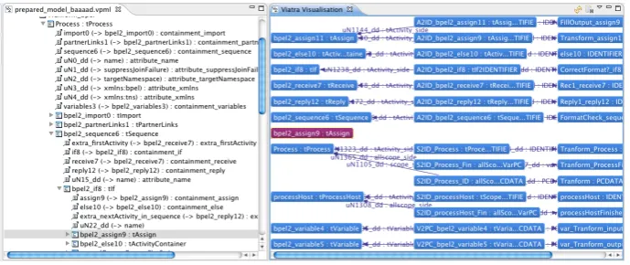
The implemented visualization component is depicted inFigure 5: next to the

containment-based display the graph viewer shows the traceability model using the proposed layout algorithm.

Figure 5: The Visualization of an Erroneous Traceability Record

Traceability Visualization in Transformation DebuggingOur traceability visualization helps

the manual uses of traceability, such as the ones defined inSection 3, as the traceability links are

displayed explicitly. The fact that the visualization is integrated into the transformation IDE helps debugging transformation programs by the easy detection of erroneous traceability links.

It is possible to detect missing (or maybe misplaced) traceability records by looking for model

elements without connections in the visualization: as the visualization ofFigure 5shows, the

(12)

The dynamic update mechanism also gives an overview of the transformation status: before the transformation is executed, only the source model is displayed, then as the transformation is executed, the trace records and the related target elements are displayed as they are created.

Our visualization layout (and component) can be used to visualize similar traceability models,

which may use different metamodels. A more detailed evaluation is available on our website1.

5 Related Work

In this section a brief overview of various initiatives in the graph visualization field is provided with special focus on model-specific visualization techniques and their use on traceability models.

VisualizationGraph drawing is a critical area of information visualization. The graph drawing

community researched layout algorithms [KW01], such as different tree layouts or algorithms

based on physical analogies such as springs or energy levels. All these algorithms can be used as the base of domain-specific layouts.

The publication information visualizer tool SHriMPBib [All03] uses domain-specific layout

algorithms by customizing the Jambalaya ontology visualization tool. Its method is similar to our approach, as filters were defined together with the settings of visual and layout parameters, but the actual design decisions were not published.

The DiaMeta editor generator framework allows specifying metamodel-dependent layout

algorithms [MM08]. The visualization is a constraint-based enhancement process: in every step it

tries to enhance the existing layout, then checks whether some metamodel-based layout constraints hold. The approach is general and flexible, especially in terms of mental map preservation after modifications, although the evaluation of the constraints could be resource-intensive.

The KIELER tool [FH10] also defines automatic layouting for graphical editors. It defines

so-called meta-layouts, that allow the application of different layouts on different parts of the diagram, and also provides a strong filtering mechanism.

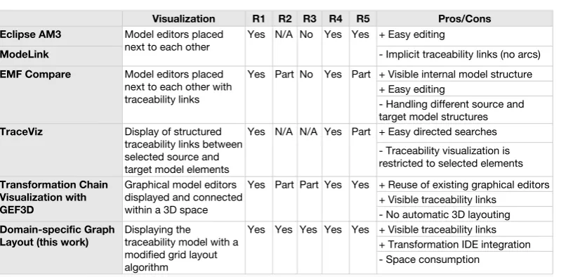
Traceability Model VisualizationWe compare several traceability model visualization

ap-proaches inFigure 6. Both the Eclipse AM3 [JVB+10] and the ModeLink [MLi] projects ease the

manual editing of trace models by putting two or three EMF editors side by side, and making it easy to add links between the editors. This approach works well for manual editing, but it is harder to get an overview of the connection between the source and target models, as the connections are

not displayed graphically but by the values of attributes. As no arcs are used, requirementR2is

not applicable, while the corresponding nodes are not grouped together (requirementR3).

The EMF Compare [BP08] project also displays the EMF editors side by side, but marks the

differences between them similarly to relations. Such a view can also be used for displaying traceability relations. In this case the entire model structure is visible in both the source and target models, but the complex structure makes it harder to get a quick overview of the traceability

relations: the nodes are not grouped together (requirementR3), and in case of different source

and target model structures it becomes hard to avoid arc crossing (requirementR2).

The TraceViz [MXP05] tool follows another approach: it displays a list of source and target

model elements, and displays the traceability links between the selected elements in a large central

(13)

Visualization R1 R2 R3 R4 R5 Pros/Cons Eclipse AM3

ModeLink

EMF Compare

TraceViz

Transformation Chain Visualization with GEF3D

Domain-specific Graph Layout (this work)

Model editors placed next to each other

Yes N/A No Yes Yes + Easy editing

- Implicit traceability links (no arcs) Model editors placed

next to each other with traceability links

Yes Part No Yes Part + Visible internal model structure + Easy editing

- Handling different source and target model structures Display of structured

traceability links between selected source and target model elements

Yes N/A N/A Yes Part + Easy directed searches - Traceability visualization is restricted to selected elements

Graphical model editors displayed and connected within a 3D space

Yes Part Part Yes Yes + Reuse of existing graphical editors + Visible traceability links

- No automatic 3D layouting Displaying the

traceability model with a modified grid layout algorithm

Yes Yes Yes Yes Yes + Visible traceability links + Transformation IDE integration - Space consumption

Figure 6: Overview of the Traceability Visualization Solutions

area. This interface allows efficient, user-directed search, but is harder to visualize changes in

this way (as the changed elements might be hidden - partial support for requirementR5). As the

connections are not displayed, requirementR2andR3cannot be applied.

The transformation chain visualization of [PVSB08] also includes a three dimensional

visual-ization of traceability links. The main idea of the approach is to put the existing model editors in a three dimensional space, and connect them with traceability links, on the other hand although the layouting options of the existing editors are reused, the traceability links are simply connect the

corresponding nodes. This way requirementR2andR3are only partially solved, as they depend

on the positioning of the editors and the camera position.

Triple Graph Grammars (TGG) are introduced in [Sch95], which also define a basic layout

that separates the three models but lacks further placement guidelines. TGGs are also used for

defining transformations in [GLMD09] include traceability information inherently, while the

VizMODLE tool supports the visualization of correspondence structures. However these do not include specific layouting for traceability models, therefore these approaches are not evaluated against the requirements.

6 Conclusion and Future Work

In case of complex model transformations (e.g. for automatic model analysis) debugging and back-annotation of the transformation necessitates the visualization of traceability connections between the source and target models in an intuitive, easy to understand way. Unfortunately generic purpose graph layout algorithms frequently fail to properly display the underlying logical structure of traceability models. To solve this problem we proposed a semi-automatic technique with domain-specific layouting by customizing generic and parameterized layout algorithms, and introduced our techniques on the BPEL2SAL case study.

(14)

we plan to investigate how to identify the structure of the source and target models, and use this information to make the visualization more intuitive.

Another extension of our proposed layout is the visualization of traceability chains: by putting the further model elements into new columns, it is possible to visualize entire traces. The main

challenge using this approach is to reduce the number of arc crossings (requirementR2), for that

an enhanced ordering method is required.

Bibliography

[AD07] M. Alessandrini, D. Dost. SENSORIADeliverable D8.3.a: Finance Case Study:

Re-quirements modelling and analysis of selected scenarios. Technical report, S&N AG, August 2007.

[All03] M. M. Allen. Empirical Evaluation of a Visualization Tool for Knowledge Engineering.

Master’s thesis, University of Victoria, 2003.

[BP08] C. Brun, A. Pierantonio. Model differences in the eclipse modelling framework.

UP-GRADE, The European J. for the Informatics ProfessionalIX(2):29–34, Apr. 2008.

[Bul08] I. Bull.Model Driven Visualization: Towards A Model Driven Engineering Approach

For Information Visualization. Ph.D. thesis, University of Victoria, BC, Canada, 2008.

[DKPF09] N. Drivalos, D. Kolovos, R. Paige, K. Fernandes. Engineering a DSL for Software

Traceability. InSoftware Language Engineering. Pp. 151–167. Springer Berlin /

Hei-delberg, 2009.

[ELMS91] P. Eades, W. Lai, K. Misue, K. Sugiyama. Preserving the mental map of a diagram. InProceedings of COMPUGRAPHICS. Volume 91, p. 2433. 1991.

[FH10] H. Fuhrmann, R. von Hanxleden. Taming Graphical Modeling. In Petriu et al. (eds.),

Model Driven Engineering Languages and Systems. Lecture Notes in Computer Sci-ence 6394, pp. 196–210. Springer Berlin / Heidelberg, 2010.

[GHV10] L. Gönczy, Á. Hegedüs, D. Varró. Methodologies for Model-Driven Development

and Deployment: an Overview. In Wirsing (ed.),Rigorous Software Engineering for

Service-Oriented Systems: Results of theSENSORIAproject on Software Engineering for Service-Oriented Computing. Springer-Verlag, 2010. To appear.

[GLMD09] E. Guerra, J. de Lara, A. Malizia, P. D´ıaz. Supporting user-oriented analysis for

multi-view domain-specific visual languages. Information & Software Technology

51(4):769–784, 2009.

[HBRV10] Á. Hegedüs, G. Bergmann, I. Ráth, D. Varró. Back-annotation of Simulation Traces

with Change-Driven Model Transformations. InProceedings of the Eigth International

(15)

[JVB+10] F. Jouault, B. Vanhooff, H. Bruneliere, G. Doux, Y. Berbers, J. Bezivin. Inter-DSL

coordination support by combining megamodeling and model weaving. InProc. of the

2010 ACM Symposium on Applied Computing. Pp. 2011–2018. 2010.

[KW01] M. Kaufmann, D. Wagner.Drawing Graphs. Lecture Notes in Computer Science

Vol-ume 2025/2001. Springer Berlin / Heidelberg, 2001.

[MLi] The ModeLink Project.http://www.eclipse.org/gmt/epsilon/doc/modelink/.

[MM08] S. Maier, M. Minas. A Generic Layout Algorithm for Meta-model Based Editors. In

Applications of Graph Transformations with Industrial Relevance. Volume Volume 5088/2008, pp. 66–81. Springer Berlin / Heidelberg, Oct. 2008.

[MXP05] A. Marcus, X. Xie, D. Poshyvanyk. When and how to visualize traceability links? In

Proceedings of the 3rd international workshop on Traceability in emerging forms of software engineering. Pp. 56–61. ACM, Long Beach, California, 2005.

[OAS07] OASIS. Web Services Business Process Execution Language Version 2.0 (OASIS

Standard). 2007.”http://docs.oasis-open.org/wsbpel/2.0/wsbpel-v2.0.html”.

[Pur97] H. Purchase. Which aesthetic has the greatest effect on human understanding? In

Graph Drawing. Lecture Notes in Computer Science, pp. 248–261. Springer Berlin / Heidelberg, 1997.

[PVSB08] J. von Pilgrim, B. Vanhooff, I. Schulz-Gerlach, Y. Berbers. Constructing and

Vi-sualizing Transformation Chains. InModel Driven Architecture Foundations and

Applications. Pp. 17–32. 2008.

[R ÖV09] I. Ráth, A. Ökrös, D. Varró. Synchronization of Abstract and Concrete Syntax in

Domain-specific Modeling Languages.Journal of Software and Systems Modeling,

2009.

[Sch95] A. Sch¨urr. Specification of Graph Translators with Triple Graph Grammars. InWG

’94: Proceedings of the 20th International Workshop on Graph-Theoretic Concepts in Computer Science. Pp. 151–163. Springer-Verlag, London, UK, 1995.

[SEN05] SENSORIA(Software Engineering in Service-Oriented Overlay Computers) EU FP6

Project. 2005.http://sensoria-ist.eu.

[Sha00] N. Shankar. Symbolic Analysis of Transition Systems. In Gurevich et al. (eds.),ASM

2000. LNCS 1912, pp. 287–302. Springer-Verlag, Monte Verit`a, Switzerland, 2000.

[V2] VIATRA2 Model Transformation Framework.http://www.eclipse.org/gmt/VIATRA2/.

[VP03] D. Varr´o, A. Pataricza. VPM: A visual, precise and multilevel metamodeling framework

for describing mathematical domains and UML.Journal of Software and Systems

Modeling2(3):187–210, October 2003.

[XLW08] K. Xu, Y. Liu, C. Wu. BPSL Modeler – Visual Notation Language for Intuitive Business