Multi-objective chance constrained transportation problem with fuzzy parameters

Multi-objective chance constrained transportation

problem with fuzzy parameters

Surapati Pramanik

Department of Mathematics, Nandalal Ghosh B.T. College,

P.O.-Panpur, Dist-North 24

Parganas, W.B., India

Durga Banerjee

Ranaghat Yusuf Institution,

Ranaghat, Dist. Nadia, West Bengal,

India

Bibhas C. Giri

Jadavpur University, Kolkata, West Bengal,

India

ABSTRACT

This paper deals with multi-objective chance constrained transportation problems. The coefficients of each objective function are considered as fuzzy numbers. The inequality constraints describing supplies and demands are stochastically defined. In the model formulation, objective functions are converted into the functions with crisp coefficients by using α-cut method (Lee and Li, 1993). Supplies and demands related chance constraints are transformed into equivalent deterministic constraints with the help of known distribution function. Then the membership functions are formulated by considering individual best solution. In the solution process, two fuzzy goal programming models are proposed. Lastly, Euclidean distance function is considered to identify the best compromise solution based on the solutions obtained from two fuzzy goal programming models. The efficiency of proposed approach is demonstrated by solving a numerical example.

General Terms

Optimization, modeling, decision making.

Keywords

Transportation Problems, Fuzzy Numbers, α-cut, Chance Constrained Programming, Fuzzy Goal Programming, Membership Function, Distribution Function.

1.

INTRODUCTION

solve MOTP with fuzzy coefficients. In the solution process, they proposed two FGP models. In 2008, Pramanik and Roy [14] studied priority based FGP for multi-objective transportation model with fuzzy parameters. Sensitivity analysis to the solution with the change of priorities of fuzzy goals was performed.

In the present paper, we consider chance constrained multi-objective transportation problem (CCMOTP) with fuzzy parameters. Here, the coefficients of the objective functions are taken as fuzzy numbers. Using Lee and Li’s [15] α-cut method (1993), the fuzzy coefficients of objective functions are transformed into crisp coefficients. The supplies and demands constraints are defined as chance constraints. With the help of given distribution function, chance constraints are transformed into equivalent deterministic constraints. In the model formulation, fuzzy goals for objective functions are suggested first. Then membership functions are constructed. For the solution, we use two FGP models which minimize only negative deviational variables. Euclidean distance function is applied to select the appropriate solution.

This paper is designed in the following ways:

In Section 2, some relevant definitions are stated. In Section 3, chance constrained multi-objective transportation problem with fuzzy parameters is described. Chance constraints are converted into equivalent deterministic constraints in the Section 4. In Section 5, fuzzy goal and membership function for each objective function are constructed. Section 6 is devoted to formulate two FGP models to solve the CCMOTP. Application of Euclidean distance function is discussed in Section 7. In Section 8, the summary of the proposed approach is described. A numerical example is solved in Section 9. The paper is concluded in Section 10 providing future scope of research.

2.

SOME RELEVANT DEFINITIONS

In this section, we state some well known definitions which are relevant in this territory.

2.1 Definition

Fuzzy Set and Membership Function: A fuzzy set A~ in X is defined by A~ = {(x, _A~ (x))  xX},where A~

 (x): X 

[0, 1] is called the membership function of A~ and _A~ (x) is the degree of membership to which xA

~

2.2 Definition

Normal Fuzzy Set: A fuzzy set A~ is said to be a normal fuzzy set if there exists at least one point x in X such that _A~ (x)

= 1. Otherwise, the set A~ is said to be a subnormal fuzzy set.

2.3 Definition

Convex Fuzzy Set: A fuzzy set A~ is said to be a convex fuzzy set if for any x and1 x2 X and[0,1],

)] x ( ), x ( [ min ] x ) 1 ( x

[ 1 2 A~ 1 A~ 2

A~      

 .

2.4 Definition

- cut: The - cut of a fuzzy set A~ of X is defined as A~[x:~_A(x),(0,1),xX]

2.5 Definition

Fuzzy Number: A fuzzy number is a normal and convex fuzzy set of real line R.

2.6 Definition

Trapezoidal Fuzzy Number: A trapezoidal fuzzy number can be defined by the foursome

) r , r , r , r (

4 4 3 3 4 4 3 2 2 1 1 2 1 1 R ~ r ≥ r , 0 r ≤ r ≤ r , r -r r -r r ≤ r ≤ r , 1 r ≤ r ≤ r , r -r r -r r ≤ r , 0 = ) r ( μ

The - cut of trapezoidal fuzzy number can be written by the interval R~[R~L,R~U][(r₂r₁)r₁,r₄(r₄r₃)] .

2.7 Definition

Triangular Fuzzy Number: A triangular fuzzy number is the triplet R~(r1,r2,r3)with the membership function defined

as: 3 3 2 2 3 3 2 2 1 1 2 1 1 R~ r r , 0 r ≤ r ≤ r , r -r r -r r r , 1 r ≤ r ≤ r , r -r r -r r ≤ r , 0 ) r (    

The - cut of the triangular fuzzy number can be written by the interval R~ [ R~ , R~ ] [(r2 r1) r1,r3 (r3 r2) ]

U

L      

  



.

3.

CONSTRUCTION OF CCMOTP WITH FUZZY PARAMETERS

Consider the following CCMOTP with trapezoidal fuzzy numbers.

Min  

  m i n 1 j ij 4 k ij 3 k ij 2 k ij 1 k ij

k(X) (C ,C ,C ,C )x

Z ~

,

k = 1, 2, …, K (1)

subject to

P ( n _i

1 j xija



 ) ≥ 1- i_, i = 1, 2, …, m (2)

P (m _j

1 i xij b



 ) ≥ 1-



j_, j = 1, 2, …, n (3)

0 < i< 1, 0 <



j< 1, (4) 0

xij (5)

P (.) means the probability of (.).

Here, we consider K objective functions, m origins and n destinations. ( k4 ij 3 k ij 2 k ij 1 k

ij,C ,C ,C

C ) is the penalty to transport a

unit of product from source i to destination j. xijbe the quantity shipped from i- th origin to j-th destination. i,



j are

Suppose C~be the - cut of a fuzzy trapezoidal number ~C(C1,C2,C3,C4)

and_C~L

,_C~U

are the lower and upper

bound of the - cut of C~.Then C~L C1(C2C1)

and C~U C4(C4C3)

.

According to Lee and Li (1993), the minimization type objective functions are replaced by the lower bound of its - cut

i.e. if L k Z ~  , U k Z ~ 

be the lower and upper limits of the objective function Z~k(X), then the equation (1) reduces to

ij m 1 i n 1 j 1 k ij 2 k ij 1 k ij L

k [C (C C ) ]x

Z~ 

 

 _{   }

(6)

And for the maximization type problem, objective function is replaced by the upper bound of its - cut i.e.

ij m 1 i n 1 j 3 k ij 4 k ij 4 k ij U

k [C (C C ) ]x

Z

~ _

 

 _{   }

(7)

Then our present problem reduces to

Min ij m 1 i n 1 j 1 k ij 2 k ij 1 k ij L

k [C (C C ) ]x

Z ~     _{   } ,

k = 1, 2, …, K, 0 <



< 1, subject to

P ( i

n 1 j xija



 ) ≥ 1- i_,

P (m _j

1 i xij b



 ) ≥ 1-



j_,

0 < i< 1, 0 <



j< 1, 0

xij where i = 1, 2, …, m, j = 1, 2, …, n (8)

4.

FORMULATION OF EQUIVALENT DETERMINISTIC CONSTRAINTS

Supplies and demands related chance constraints of the type P ( i n

1 j xija



 ) ≥ 1- i, i = 1, 2, …, m

can be written as:

P ( ) a var( ) a ( E a ) a var( ) a ( E x i i i i n 1

j ij i  

 

) ≥ 1- i_,

i = 1, 2, …, m

  

 _i 1 P (

) a var( ) a ( E a ) a var( ) a ( E x i i i i n 1

j ij i  

 

),

i = 1, 2, …, m

) ) a var( ) a ( E a ) a var( ) a ( E x ( P i i i i n 1

j ij i i        ,

    ) ( F i 1 ) a var( ) a ( E x i n 1

j ij i



  _{, i = 1, 2, …, m}

 

 _{  }

 n

1

j ij i i i 1 ) a ( E x ) a var( ) (

F , i = 1, 2, …, m

   _    n 1

j i i

1 i

ij E(a ) F ( ) var(a )

x ,

i = 1, 2, …, m (9)

where F (.) and F-1 (.) represent respectively the distribution function and inverse of distribution function.

Supplies and demands related chance constraints of the type P(m _j 1 i xijb



 ) ≥ 1-



j, j = 1, 2, …, n

can be written as:

P ( ) b var( ) b ( E b ) b var( ) b ( E x j j j j j m 1

i ij  



 _{) ≥}

1-j



,

j = 1, 2, …, n

j

j j m

1

i ij _{) 1}

-) b var( ) b ( E x (

F   

  _{, j = 1, 2, …, n}

j j j m 1 i ij -1 ) ) b var( ) b ( E x (-F

1   

  _{, j = 1, 2, …, n}

j j

j m

1

i ij ₎

) b var( ) b ( E x

(-F  

  _{, j = 1, 2, …, n}

) b var( ) b ( E x ) ( F j j m 1 i ij j

1   

  

, j = 1, 2, …, n

) b var( ) b ( E x ) ( F j j m 1 i ij j

1   



   _{, j = 1, 2, …, n}

   _    m 1

i j j

1 j

ij E(b ) F ( ) var(b )

x ,

j = 1, 2, …, n (10)

Then the problem (1) reduces to

Min m _ij

1 i n 1 j 1 k ij 2 k ij 1 K ij L

k [C (C C ) ]x

Z ~     _{   } ,

k = 1, 2, …, K (11)

subject to    _   n 1

j i i

1 i

ij E(a) F ( ) var(a)

   _   m 1

i j j

1 j

ij E(b ) F ( ) var(b )

x (13)

The deterministic constraints (5), (12) and (13) are denoted by S.

5.

CONSTRUCTION OF FUZZY GOAL AND MEMBERSHIP FUNCTION

The k-th objective function is L k

Z ~



which represents either TP cost or time or damages during transportation. Our

problem is to minimize L k

Z ~



subject to the system constraints (12), (13) and (5). Let the individual best and worst value

of the objective function subject to system constraints be L k B

Z and U

k W

Z respectively where S ∈ x Min L k Z ~  = L k B

Z and S ∈ x Max U k Z~  = U k W

Z . The fuzzy goals appear as L k Z ~ 

~



L k B

Z , k = 1, 2, …, K. The membership function μ ( Z~L)

k α

k for the k-th

fuzzy goal can be constructed as follows:

U k W L k U k W L k L k B L k B U k W L k U k W L k B L k L k k Z ≥ Z ~ if , 0 Z ≤ Z ~ ≤ Z if , Z -Z Z ~ -Z Z ≤ Z ~ if , 1 ) Z ~ (      _  ,

k = 1, 2, …, K

(14)

Using the concept of Pramanik and Roy [16] and Pramanik and Dey [17], the corresponding membership goals for membership functions can be written as



 _

 k

L k k Z ) d

~

( = 1, k = 1, 2, …, K (15)

where dk is the negative deviational variable.

6.

FGP MODEL FORMULATION

New FGP models for CCMOTP with fuzzy parameter are given below:

6.1

FGP model I a

For prescribed value of, the FGP model can be presented as follows:

Min  





 K _k

1

k wkd

subject to 

 _

 L _k

k k Z ) d

~

( = 1,

1 d 0 k 

 _{, k = 1, 2, …, K}

S

X

where wk = 1/(

L k B U k W Z

Z  ) (16)

The numerical weight wk represents the associated weight for the k- th negative deviational variable.

6.2

FGP model I b

Min  =   K 1 k k d subject to   _

 L _k

k k Z ) d

~

1 d 0 k 

 _{, k = 1, 2, …, K}

S

X (17)

6.3

FGP model II

Min

subject to

 _≥ 

k

d ,



 _

 L _k

k k Z ) d

~

( = 1,

1 d 0 k 

 _{, k = 1, 2, …, K}

S

X (18)

7.

USE OF EUCLIDEAN DISTANCE FOR BEST COMPROMISE SOLUTION

We use two FGP models to solve the problem (1). In multi-objective decision making situation, we are not able to reach the ideal solution point of each objective function. Then our motto is to obtain such a solution for which overall regrets will be minimal. Euclidean distance function [17] is applied to detect the satisfactory solutions obtained from two FGP models. The Euclidean distance function can be defined as follows:

D=



K



1/2

1 k

2 L k k

)) Z ~ ( 1 (

 





 . (19)

Minimum value of the distance function D will represent the best compromise solution.

8.

SUMMARY

To solve the CCMOTP with fuzzy parameters, the following steps are followed.

Step 1: First we convert the fuzzy coefficients of the objective functions into equivalent crisp coefficients.

Step 2: In the next step we transform the chance constraints into equivalent deterministic constraints.

Step 3: After determining individual the best and worst solutions as the lower and upper bounds, we formulate the membership functions.

Step 4: In the next step, we formulate two FGP models.

Step 5: In the next step, we solve the two FGP models.

Step 6: Euclidean distance is calculated for the solutions obtained from two FGP models.

Step 7: The solution having least Euclidean distance is chosen as the compromise solution.

9.

NUMERICAL EXAMPLE

The following CCMOTP with fuzzy parameters is considered to demonstrate our approach.

Min~Z₁~5x₁₁~2x₁₂~3x₁₃8x₂₁~9x₂₂~4x₂₃, (20) Min~Z₂ 3x₁₁~4x₁₂~2x₁₃~6x₂₁~3x₂₂1~5x₂₃, (21)

P ( 3 ₁ 1 j 1j

a x 



 ) ≥ 1-1, (23)

P ( 3 ₂

1 j x2ja



 ) ≥ 1-2_, (24)

P ( 2 ₁

1 i xi1b



 ) ≥ 1- 1_, (25)

P ( 2 ₂

1 i xi2b



 ) ≥ 1- 2 , (26)

P ( 3

2 1 i xi3b



 ) ≥ 1- 3_, (27)

xij ≥ 0 , i = 1, 2 and j = 1, 2, 3. (28)

The mean, variance and the confidence levels are described below:

E (a1) = 20, var (a1) = 4, α1= 0.01

E (a2) = 5, var (a2) = 2, α2= 0.03

E (b1) = 16, var (b1) = 9, β1= 0.02

E (b2) = 8, var (b2) = 3, β2= 0.05

E (b3) = 25, var (b3) = 16, β3= 0.02

The triangular fuzzy coefficients are~5=[4,5,6],~2=[1,2,3],~3=[2,3,4],~9=[8,9,10],~4=[3,4,5],~6=[4,6,8], 15~=[14,15,16], ] 14 , 12 , 10 [ = 2 ~

1 , 7~=[6,7,8],1~4=[12,14,16].

Using (9), (10) the chance constraints defined in (23) to (27) are converted into equivalent deterministic constraints as follows:

65 . 24 ≤

∑3_x

1 = j 1j

,∑x ≤7.67

3 1 = j 2j

, ∑2_x ≥9.835 1

= i i1

,∑2_x ≥5.15 1

= i i2

,∑3_x ≥16.78 1

= i i3

(29)

Using (11), the objective functions are transformed as follows:

Min L 1 Z ~  23 22 21 13 12

11 (1 )x (2 )x 8x (8 )x (3 )x x

) 4

(          

 (30)

Min L 2 Z ~  23 22 21 13 12

11 (3 )x (1 )x (4 2 )x (2 )x (14 )x x

3           

 (31)

Min L 3 Z~  23 22 21 13 12

11 (6 )x (12 2 )x (1 )x (4 )x x x

) 2 10

(            

 (32)

Then for prescribed value of



(0 <



< 1), the proposed CCMOTP reduces to

Min L k

Z~



k = 1, 2, 3.

subject to 65 . 24 x 3 1 j 1j



 , x 7.67

3 1 j 2j



 , x 9.835

2 1 i i1



 , x 5.15

2 1 i i2



 , x 16.78

3 1 i i3





Now the FGP models defined in (16), (17), (18) are solved for different values of α and all results are shown in the table 1.

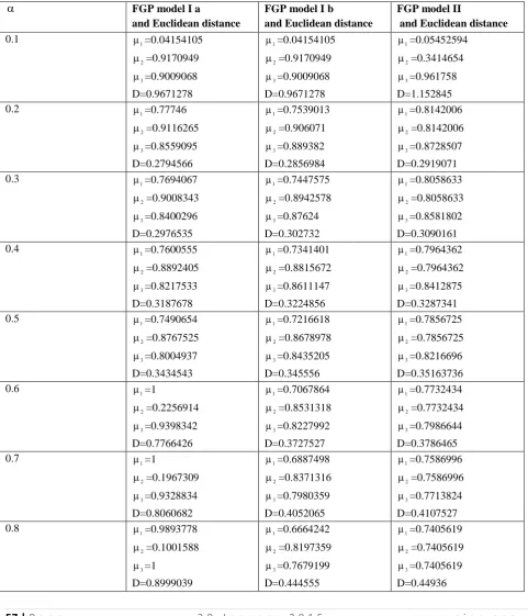
Table 1 Membership functions with Euclidean distance



α FGP model I a and Euclidean distance

FGP model I b and Euclidean distance

FGP model II

and Euclidean distance

0.1 ₁=0.04154105

2  =0.9170949 3  =0.9009068 D=0.9671278 1  =0.04154105 2  =0.9170949 3  =0.9009068 D=0.9671278 1  =0.05452594 2  =0.3414654 3  =0.961758 D=1.152845

0.2 ₁=0.77746

2  =0.9116265 3  =0.8559095 D=0.2794566 1  =0.7539013 2  =0.906071 3  =0.889382 D=0.2856984 1  =0.8142006 2  =0.8142006 3  =0.8728507 D=0.2919071

0.3 ₁=0.7694067

2  =0.9008343 3  =0.8400296 D=0.2976535 1  =0.7447575 2  =0.8942578 3  =0.87624 D=0.302732 1  =0.8058633 2  =0.8058633 3  =0.8581802 D=0.3090161

0.4 ₁=0.7600555

2  =0.8892405 3  =0.8217533 D=0.3187678 1  =0.7341401 2  =0.8815672 3  =0.8611147 D=0.3224856 1  =0.7964362 2  =0.7964362 3  =0.8412875 D=0.3287341

0.5 ₁=0.7490654

2  =0.8767525 3  =0.8004937 D=0.3434543 1  =0.7216618 2  =0.8678978 3  =0.8435205 D=0.345556 1  =0.7856725 2  =0.7856725 3  =0.8216696 D=0.35163736

0.6 ₁=1

2  =0.2256914 3  =0.9398342 D=0.7766426 1  =0.7067864 2  =0.8531318 3  =0.8227992 D=0.3727527 1  =0.7732434 2  =0.7732434 3  =0.7986644 D=0.3786465

0.7 ₁=1

2  =0.1967309 3  =0.9328834 D=0.8060682 1  =0.6887498 2  =0.8371316 3  =0.7980359 D=0.4052065 1  =0.7586996 2  =0.7586996 3  =0.7713824 D=0.4107527

0.8 ₁=0.9893778

0.9 ₁=0.9879445

2

 =0.06283278

3

 =1 D=0.9372448

1

 =0.6380737

2

 =0.8007536

3

 =0.7305055 D=0.4932718

1

 =0.7140385

2

 =0.7140385

3

 =0.7140385 D=0.4952998

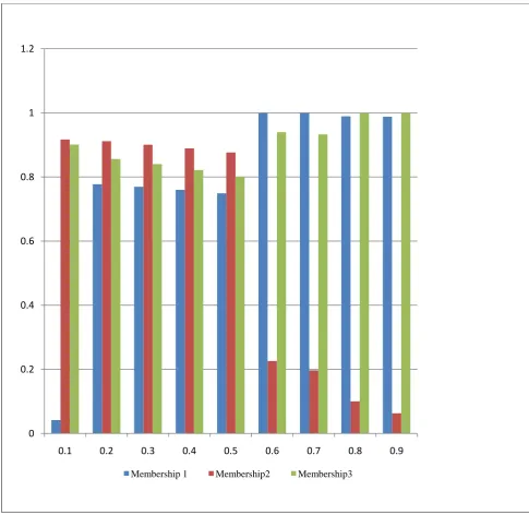
The obtained values of three membership functions for each value of α are depicted by the bar diagrams for the three models.

Fig 1:The obtained values of three membership functions for each value of α for the model I a

0 0.2 0.4 0.6 0.8 1 1.2

0.1 0.2 0.3 0.4 0.5 0.6 0.7 0.8 0.9

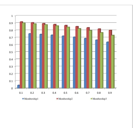
Fig 2: The obtained values of three membership functions for each value of α for model I b 0

0.1 0.2 0.3 0.4 0.5 0.6 0.7 0.8 0.9 1

0.1 0.2 0.3 0.4 0.5 0.6 0.7 0.8 0.9

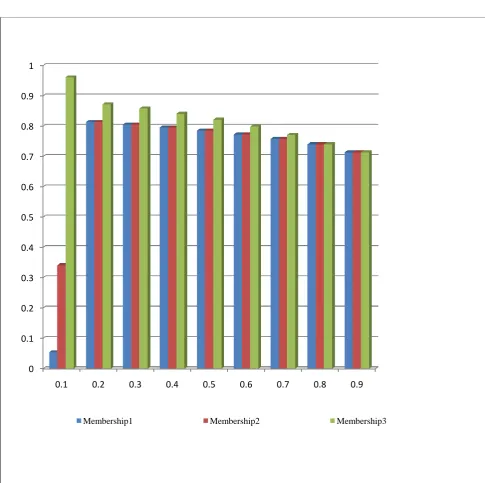
Fig 3: The obtained values of three membership functions for each value of α for the model II.

The distance values obtained from three FGP models for each value of α are plotted in the following bar diagram.

0 0.1 0.2 0.3 0.4 0.5 0.6 0.7 0.8 0.9 1

0.1 0.2 0.3 0.4 0.5 0.6 0.7 0.8 0.9

Comparing the height of the bar, the best compromise solution occurs with least height of the bar.

10.

CONCLUSION

In this paper, chance constrained multi-objective transportation problem with fuzzy parameters is studied. In real life situation, it is not always possible to describe the exact value of penalties for transportation. So, fuzzy parameters are used to describe penalties. In TP, it is noticed that capacity of origin and the demand of destination are random in nature. In this study, the inequality constraints describing supplies and demands are stochastically defined. Two new FGP models are formulated for solving multi-objective chance constrained transportation problem with fuzzy parameters. Euclidean distance function is applied to identify best compromise solution. It is hoped that the proposed approach can be extended for chance constrained bi-level as well as multi- level transportation problems.

11.

ACKNOWLEDGMENTS

Our thanks to the experts who have contributed towards development of the template.

12.

REFERENCES

0 0.1 0.2 0.3 0.4 0.5 0.6 0.7 0.8 0.9 1 1.1 1.2 1.3 1.4 1.5

0.1 0.2 0.3 0.4 0.5 0.6 0.7 0.8 0.9

[1] Hitchcock, F. L. 1941. The distribution of a product from several sources to numerous localities. Journal of Mathematical Physics, 20(1), 224–230.

[2] Koopmans, T. C. Activity analysis of production and allocation. Cowels Commission Monograph, Wiley, New York, 13.

[3] Charnes, A. and Cooper, W. W. 1954. The stepping stone method for explaining linear programming calculation in transportation problem.Management Science, 1(1), 49-69.

[4] Wagner, H. M. 1959. ON a class of capacitated transportation problems. Management Science, 5(3), 304-318.

[5] Kantorovitch, L. V. 1960. Mathematical methods in the organization and planning of production. Publication House of the Leningrad State University (in Russian Language), English translation in Management Science, 6(4), 366 – 422.

[6] Haley, K. B. 1963. The solid transportation problem. Operation Research,10(4), 448-463.

[7] Isermann, H. 1979. The enumeration of all efficient solutions for a linear multi-objective transportation problem. Naval Research. Logistic, Quarterly, 26(1), 123139.

[8] Ringuest, J. L. and Rinks, D. B. 1987. Interactive solutions for the linear multi-objective transportation problem. European Journal of Operational Research, 32(1), 96-106.

[9] Bit, A. K., Biswal, M. P. and Alam, S. S. 1992. Fuzzy programming approach to multi-criteria decision making transportation problem. Fuzzy Sets and Systems, 50(2), 135-141.

[10] Li, L. and Lai, K. K. 2000. A fuzzy approach to multi-objective transportation problem. Computers and Operations Research, 27(1), 43–57.

[11] Gao, S. P. and Liu, S. A. 2004. Two-phase fuzzy algorithms for multi-objective transportation problem. The Journal of Fuzzy Mathematics, 12(1), 147-155.

[12] Abd El-Wahed, W. F. and Lee, S. M. 2006. Interactive fuzzy goal programming for multi-objective transportation problems. Omega, 34(2), 158-166.

[13] Pramanik, S. and Roy, T. K. 2006. A fuzzy goal programming technique for solving multi-objective transportation problem. Tamsui Oxford Journal of Management Science, 22(1), 67-89.

[15] Lee, E. S. and Li, R. J. 1993. Fuzzy multiple objective programming and compromise programming with Pareto optimum. Fuzzy Sets and Systems, 53(2), 275–288.

[16] Pramanik, S. and Roy, T. K. 2007. Fuzzy goal programming approach to multilevel programming problems. European Journal of Operational Research, 176(2), 1151-1166.