Identifying Effective Features
and Classifiers for Short Term
Rainfall Forecast Using Rough Sets
Maximum Frequency Weighted
Feature Reduction Technique
Sudha Mohankumar
1and Valarmathi Balasubramanian
21Information Technology Department, School of Information Technology and Engineering, VIT University, Vellore, India 2Software and Systems Engineering Department, School of Information Technology and Engineering, VIT University,
Vellore, India
Precise rainfall forecasting is a common challenge across the globe in meteorological predictions. As rainfall forecasting involves rather complex dy-namic parameters, an increasing demand for novel approaches to improve the forecasting accuracy has heightened. Recently, Rough Set Theory (RST) has at-tracted a wide variety of scientific applications and is extensively adopted in decision support systems. Al-though there are several weather prediction techniques in the existing literature, identifying significant input for modelling effective rainfall prediction is not ad-dressed in the present mechanisms. Therefore, this in-vestigation has examined the feasibility of using rough set based feature selection and data mining methods, namely Naïve Bayes (NB), Bayesian Logistic Re-gression (BLR), Multi-Layer Perceptron (MLP), J48, Classification and Regression Tree (CART), Random Forest (RF), and Support Vector Machine (SVM), to forecast rainfall. Feature selection or reduction process is a process of identifying a significant feature subset, in which the generated subset must characterize the information system as a complete feature set. This pa-per introduces a novel rough set based Maximum Fre-quency Weighted (MFW) feature reduction technique for finding an effective feature subset for modelling an efficient rainfall forecast system. The experimen-tal analysis and the results indicate substantial im-provements of prediction models when trained using the selected feature subset. CART and J48 classifiers have achieved an improved accuracy of 83.42% and 89.72%, respectively. From the experimental study, relative humidity2 (a4) and solar radiation (a6) have been identified as the effective parameters for model-ling rainfall prediction.
ACM CCS (2012) Classification: Computing
meth-odologies → Machine learning → Machine learning algorithms → Feature selection;
Information systems → Information retrieval → Re
-trieval tasks and goals → Clustering and classification; Applied computing → Operations research → Fore -casting
Keywords: rainfall prediction, rough set, maximum frequency, optimal reduct, core features and accuracy
1. Introduction
pro-posed model could predict rainfall in significant consistency with real measurements. [3] de-scribed a feature selection approach using ge-netic algorithm for heavy rainfall predictions in South Korea. They used weather data collected from European Medium Range Weather Fore-cast centre between 1989 and 2009. Despite the existence of several works related to rainfall prediction, there is always a demand for better techniques for prediction due to the magnitude of impact rainfall has on the environment. The foremost intent of this research is to accom-plish improved prediction accuracy through the use of effective weather parameters using proposed rough set feature selection and data mining methods. This research is different from previous work as it delves into identifying the influencing features that enable efficient rain-fall forecast. The proposed model not only fo-cuses on feature reduction but also on finding a list of parameters contributing to precision instead of just finding a subset or attaining di-mensionality reduction.
2. Foundation
Rough Set Theory (RST), as proposed by Z. Pawlak in 1982, is a mathematical model that deals with vague and imperfect knowledge. RST does not require any prior knowledge or additional information about the data [4] [5] [6]. In rough set, data analysis starts from a ta-ble referred to as decision or information tata-ble representing an information system. Rough set having a wide scope has been adopted in a wide range of scientific and medical applications, es-pecially in the field of pattern recognition, data mining, machine learning, process control and knowledge representation systems [7] [8] [9]. Rough sets have been used in various medical, meteorological applications for knowledge dis-covery [10].
Definition 1. Information System
Let an information system be I = {X, A, V, S}, where X is a universal set that constitutes the domain objects of the system. { } {A → C D∪
}
is a feature set that includes condition features and the decision feature. V→(
VrXr∈ R rV)
is a set of features. Vr is the feature value range of:. X
r AS∈ × →A V is an information function, which designates each object feature value in V that constitutes an information system.
Definition 2. Decision Table
It is a finite set of objects that constitute an in-formation system description represented as a table. The decision table consists of a finite set of conditional and decision features. The sam-ple information table of this rainfall forecast system is presented in Table 1. The dataset has eight conditional attributes or features repre-sented as (a1, a2, a3, a4, a5, a6, a7, and a8) and one decision variable (Rf).
Definition 3. Approximation Space
In an information system I = {X, A, V, S}, the rough set concept can be defined by means of topological operations, i.e., interior and closure, called approximations. The key concept of the presented rough set approach is the mathemat-ical formulation of the concept of equality of sets defined as approximation space [6].
Definition 4. Discernible and Indiscernible Re-lation
For an information system I = (O, A), O → {} is a non-empty set of objects and A → {} a non-empty set of features where each {SA} → subset of features of {A}. 'R' is the equivalence relation called indiscernibility re-lation on the set {I} that contains the elements with similar feature values and complements of it as discernible relation. This equivalence re-lation partitions the universe to several classes and union of all equivalence relations form the set {I}. The equivalence class of R determined by element x is denoted by R(x).
Definition 5. Lower and Upper Approximation Let I = (U, A) and let B ⊆ A and X ⊆ U, we can approximate X using only the informa-tion obtained in B by constructing the B-lower and B-upper approximations of X denoted as BX and BX, respectively. A lower approxi-mation set of X is the set of all elements of U that are certainly classified as elements of X, where BX=
{
x| x[ ]
B⊆ X}
. Upper approxima-tion set of X contains all data which can pos-sibly be classified as belonging to the set X is[ ]
{
B}
BX= x| x ∩X≠ϕ . Approximation
accu-racy is determined using the lower and upper approximation space.
Definition 6. Reduct and Core
The two fundamental concepts of RST are core and reduct. The reduct set {R} is the indispens-able part of an information system with all pos-sible subsets of features. Reduct set can discern all objects as a complete feature set {A}. The core is the indispensable feature of reducts, where
{ } { } { }
{ }
Core= R1 ∩ R2 ∩ R3 ...∩ Rn (1) The proposed rough set based Maximum Fre-quency Weighted (MFW) feature reduction model is designed based on RST. This model is used to reduce the feature space of meteoro-logical (rainfall) dataset and to identify the sig-nificant features. Initially, the required possible combinations of feature reduct sets are gener-ated using Rosetta (http://rosetta.org), which is an open source Rough Set Toolkit for data analysis (Rosetta) [11]. The required target in-put for the proposed algorithm is determined using Rosetta's genetic algorithm based feature reduction technique. These sets of reducts are then used in identifying the effective features based on the novel feature ranking based fre-quency weighted feature reduction approach. In the next phase, the impact of succeeding set of feature subsets is evaluated based on the perfor-mance of classification models. The proposed algorithm background and implementation tails are described in subsection 5.2. The de-tailed working model and the performance out-comes are discussed in the experimental results and discussion sections.
3. Related Works
[12] proposed a feature selection approach using genetic algorithm to select key features from the complete feature set using data mining methods. They proposed an improved Naïve Bayes classifier technique and explored the use of genetic algorithms (GAs) for selecting a subset of the input features in the classification. [13] described Johnson selection algorithm and the Object Reduct using Feature Weight-ing technique (ORFW) for reduct computation. Both algorithms aim at reducing the number of
features in the dataset based on discernibility matrix. [14] described a modified binary dis-cernibility matrix for feature selection algo-rithm based on discernibility matrix that dealt directly with inconsistent decision-making sys-tem. Ordering and simple link technique in the algorithm reduced the size of the input table, which, in turn, reduced the computation and storage space. [15] reported a two-step feature selection technique. A discretisation process of reducing the domain of a continuous features with irreducible and an optimal set of cuts was adopted based on the discernibility matrix. [16] described a reduct optimization method based on the conditional features to generate representative data to simplify the discernibil-ity matrix. [17] described a reduct construction method based on discernibility matrix simpli-fication. Elements of a minimum discernibil-ity matrix are either the empty set or singleton subsets, in which the union derives a reduct using heuristic reduct algorithms. [18] inves-tigated Support Vector Machine (SVM) classi-fier as a suitable model for rainfall forecasting. [19] utilized a new fuzzy based feature selec-tion approach for a medical dataset in tumour diagnosis. In this approach, feature selection method based on the fuzzy gain ratio under the framework of fuzzy RST has been described by experiment results. They have demonstrated the effectiveness of the proposed approach by comparing the proposed approach with several other approaches on three real world tumour datasets in gene expression. This model will be useful for various medical data diagnosis. [20] proposed a new feature selection algorithm us-ing analogical matrix. The proposed algorithm can reduce time complexity and spatial com-plexity after feature selection without breaking the coherence of the information contained in the decision table.
posed model could predict rainfall in significant consistency with real measurements. [3] de-scribed a feature selection approach using ge-netic algorithm for heavy rainfall predictions in South Korea. They used weather data collected from European Medium Range Weather Fore-cast centre between 1989 and 2009. Despite the existence of several works related to rainfall prediction, there is always a demand for better techniques for prediction due to the magnitude of impact rainfall has on the environment. The foremost intent of this research is to accom-plish improved prediction accuracy through the use of effective weather parameters using proposed rough set feature selection and data mining methods. This research is different from previous work as it delves into identifying the influencing features that enable efficient rain-fall forecast. The proposed model not only fo-cuses on feature reduction but also on finding a list of parameters contributing to precision instead of just finding a subset or attaining di-mensionality reduction.
2. Foundation
Rough Set Theory (RST), as proposed by Z. Pawlak in 1982, is a mathematical model that deals with vague and imperfect knowledge. RST does not require any prior knowledge or additional information about the data [4] [5] [6]. In rough set, data analysis starts from a ta-ble referred to as decision or information tata-ble representing an information system. Rough set having a wide scope has been adopted in a wide range of scientific and medical applications, es-pecially in the field of pattern recognition, data mining, machine learning, process control and knowledge representation systems [7] [8] [9]. Rough sets have been used in various medical, meteorological applications for knowledge dis-covery [10].
Definition 1. Information System
Let an information system be I = {X, A, V, S}, where X is a universal set that constitutes the domain objects of the system. { } {A → C D∪
}
is a feature set that includes condition features and the decision feature. V→(
VrXr∈ R rV)
is a set of features. Vr is the feature value range of:. X
r AS∈ × →A V is an information function, which designates each object feature value in V that constitutes an information system.
Definition 2. Decision Table
It is a finite set of objects that constitute an in-formation system description represented as a table. The decision table consists of a finite set of conditional and decision features. The sam-ple information table of this rainfall forecast system is presented in Table 1. The dataset has eight conditional attributes or features repre-sented as (a1, a2, a3, a4, a5, a6, a7, and a8) and one decision variable (Rf).
Definition 3. Approximation Space
In an information system I = {X, A, V, S}, the rough set concept can be defined by means of topological operations, i.e., interior and closure, called approximations. The key concept of the presented rough set approach is the mathemat-ical formulation of the concept of equality of sets defined as approximation space [6].
Definition 4. Discernible and Indiscernible Re-lation
For an information system I = (O, A), O → {} is a non-empty set of objects and A → {} a non-empty set of features where each {SA} → subset of features of {A}. 'R' is the equivalence relation called indiscernibility re-lation on the set {I} that contains the elements with similar feature values and complements of it as discernible relation. This equivalence re-lation partitions the universe to several classes and union of all equivalence relations form the set {I}. The equivalence class of R determined by element x is denoted by R(x).
Definition 5. Lower and Upper Approximation Let I = (U, A) and let B ⊆ A and X ⊆ U, we can approximate X using only the informa-tion obtained in B by constructing the B-lower and B-upper approximations of X denoted as BX and BX, respectively. A lower approxi-mation set of X is the set of all elements of U that are certainly classified as elements of X, where BX=
{
x| x[ ]
B⊆ X}
. Upper approxima-tion set of X contains all data which can pos-sibly be classified as belonging to the set X is[ ]
{
B}
BX= x| x ∩X≠ϕ . Approximation
accu-racy is determined using the lower and upper approximation space.
Definition 6. Reduct and Core
The two fundamental concepts of RST are core and reduct. The reduct set {R} is the indispens-able part of an information system with all pos-sible subsets of features. Reduct set can discern all objects as a complete feature set {A}. The core is the indispensable feature of reducts, where
{ } { } { }
{ }
Core= R1 ∩ R2 ∩ R3 ...∩ Rn (1) The proposed rough set based Maximum Fre-quency Weighted (MFW) feature reduction model is designed based on RST. This model is used to reduce the feature space of meteoro-logical (rainfall) dataset and to identify the sig-nificant features. Initially, the required possible combinations of feature reduct sets are gener-ated using Rosetta (http://rosetta.org), which is an open source Rough Set Toolkit for data analysis (Rosetta) [11]. The required target in-put for the proposed algorithm is determined using Rosetta's genetic algorithm based feature reduction technique. These sets of reducts are then used in identifying the effective features based on the novel feature ranking based fre-quency weighted feature reduction approach. In the next phase, the impact of succeeding set of feature subsets is evaluated based on the perfor-mance of classification models. The proposed algorithm background and implementation tails are described in subsection 5.2. The de-tailed working model and the performance out-comes are discussed in the experimental results and discussion sections.
3. Related Works
[12] proposed a feature selection approach using genetic algorithm to select key features from the complete feature set using data mining methods. They proposed an improved Naïve Bayes classifier technique and explored the use of genetic algorithms (GAs) for selecting a subset of the input features in the classification. [13] described Johnson selection algorithm and the Object Reduct using Feature Weight-ing technique (ORFW) for reduct computation. Both algorithms aim at reducing the number of
features in the dataset based on discernibility matrix. [14] described a modified binary dis-cernibility matrix for feature selection algo-rithm based on discernibility matrix that dealt directly with inconsistent decision-making sys-tem. Ordering and simple link technique in the algorithm reduced the size of the input table, which, in turn, reduced the computation and storage space. [15] reported a two-step feature selection technique. A discretisation process of reducing the domain of a continuous features with irreducible and an optimal set of cuts was adopted based on the discernibility matrix. [16] described a reduct optimization method based on the conditional features to generate representative data to simplify the discernibil-ity matrix. [17] described a reduct construction method based on discernibility matrix simpli-fication. Elements of a minimum discernibil-ity matrix are either the empty set or singleton subsets, in which the union derives a reduct using heuristic reduct algorithms. [18] inves-tigated Support Vector Machine (SVM) classi-fier as a suitable model for rainfall forecasting. [19] utilized a new fuzzy based feature selec-tion approach for a medical dataset in tumour diagnosis. In this approach, feature selection method based on the fuzzy gain ratio under the framework of fuzzy RST has been described by experiment results. They have demonstrated the effectiveness of the proposed approach by comparing the proposed approach with several other approaches on three real world tumour datasets in gene expression. This model will be useful for various medical data diagnosis. [20] proposed a new feature selection algorithm us-ing analogical matrix. The proposed algorithm can reduce time complexity and spatial com-plexity after feature selection without breaking the coherence of the information contained in the decision table.
and experimentation, they had concluded that BCO algorithm based rough set as optimum ex-ibited consistent and better performance when compared with other methods. Therefore, they had recommended the Bee Colony Based Re-duct (BeeRSAR) approach for the numerical datasets.
[22] described an approach for reduct computa-tion based on ACO methodology. The proposed approach has three steps: (1) updated phero-mone trails are directed to the nodes that are visited by the ants rather than the edges con-necting these nodes, (2) the pheromone trail values are limited between max and min trails, (3) heuristic values are dynamically estimated during the Ant Colony based search. The out-puts of experimentation have shown that the proposed approach can produce a short reduct with fewer iterations in comparison to other ACO based feature selection approaches. [23] described the application of rough set concept for hybrid data which involved different data with imperfect knowledge, which can be han-dled efficiently using rough set. [24] described the use of rough sets concept for multi-criteria data analysis. [25] reported a new classifica-tion approach by integrating feature selecclassifica-tion algorithms to enhance predictor accuracy. [26] created a rainfall prediction model based on Bayesian classifier. In Bayesian approach, the model performed well for those datasets with predictor class label; however, in the absence of predictor class label for a given dataset, the Bayesian classification model assumed the record with zero probability thereby affecting the overall accuracy. On the other hand, [27] formulated a new reduct optimization method
based on the condition attributes to simplify the discernibility matrix and the complexity of the attribute reduction. Analogical matrix based at-tributed reduction algorithm is a new approach towards attribute reduction. Experimental eval-uation exposed that it can reduce the time com-plexity and spatial comcom-plexity without breaking the coherence of the information contained in the decision table [28].
In general, rainfall prediction is an important disaster prevention task; hence the demand for new methodologies in this field of study never subsides [29] [30]. Therefore, the main intent of this research is to identify the most influencing weather parameters using rough set approach. This proposed model is an attempt to identify the parameters that can improve the prediction efficiency of the classification models without blindly reducing the feature vector. This study introduces a novel MFW feature reduction technique for estimating the significance of the features based on ranking to enhance the pre-diction accuracy.
4. Materials and Methods
Dataset: The daily rainfall data, measured in millimetre (mm), were obtained from the de-partment of meteorology, Tamil Nadu Agricul-tural University (TNAU), Coimbatore, India. The assessment of rainfall prediction data for a period of 29 years from 1984 to 2013 consisted of observatory records of eight atmospheric parameters. The dataset had 0.5% of missing data and 0.3% of outliers in the raw dataset, which was identified and removed during data
Table 1. Daily rainfall observatory records (1984 – 2013).
a1 a2 a3 a4 a5 a6 a7 a8 Rf
Celsius Celsius % % Km/Hrs KCalories Hrs mm mm
28 14 94 55 7.4 260 10.2 3.4 0
28 18 95 51 9 232 9.4 4.2 0
28.5 18 95 42 7.4 200 8.1 4 0
28 18.5 85 46 7.4 213.6 9.6 4.8 0
28.4 23.2 88 85 7.5 200.2 1.9 3.6 1
28 23 68 60 11.8 231 0 2.3 1
33 22.7 84 74 6.4 182.4 5.3 2.6 1
32.6 20 93 34 14.1 405 8.8 7.8 1
pre-processing phase. The eight conditional variables and one decision variable in the tar-get dataset are represented as: Maximum tem-perature (a1), Minimum temtem-perature (a2), Rel-ative humidity1 (a3), RelRel-ative humdity2 (a4), Wind speed (a5), Solar radiation (a6), Sunshine (a7), Evapotranspiration (a8) and Rainfall (Rf). The rainfall (Rf) is a binary decision variable; (Rf = 0) → no rainfall and (Rf = 1) → rainfall occurrence. The sample target dataset used as input for the proposed investigation is repre-sented in Table 1.
5. Rough Set Based Feature
Selection Techniques
Rough set based feature selection techniques are of wide ranges as shown in Figure 1. The reduct sets are generated based on rough sets discernibility matrix, indiscernibility matrix using the elements of the approximation space. The algorithms used for feature selection are of three types, namely filter, wrapper, and hybrid techniques. In this model, the discernible rela-tion based wrapper technique has been adopted for feature selection.
Figure 1. Rough set based feature reduction techniques.
5.1 Input Data Selection Methodology This investigation identifies set of features as optimal feature reduct set from 'n' feature sub-sets generated using rough set genetic algorithm. The genetic algorithm is an evolutionary com-putational heuristic search that impersonates the human progression of evolution. This search strategy can generate solutions to achieve global optimization in search problems. A typical ge-netic algorithm procedure starts from the pop-ulation of completely random individuals, and then it determines the fitness of the complete population. Each generation consists of some important operations, such as selection, cross-over, mutation, and replacement. Few individu-als in the existing population are replaced with new individuals to form a new population. Fi-nally, this generational process is repeated, until a termination condition is reached. This input data selection phase introduces a novel rough set based MFW feature selection approach for computing the most relevant weather parameter for effective prediction. It is an exhaustive task having a suitable stopping criterion to terminate the selection process.
5.2. Maximum Frequency Weighted Feature Reduction Technique
MFW feature selection identifies the significant weather parameter from the complete set of
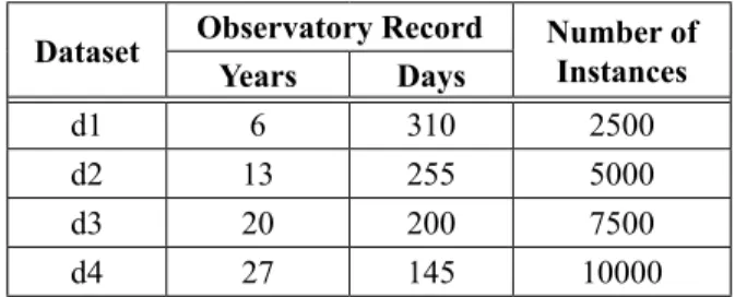
duct sets based on the individual parameters frequency ranking. The target input dataset for the proposed MFW feature selection approach is partitioned as four segments, namely d1, d2, d3, and d4 as shown in Table 2 for conducting a performance evaluation of the proposed ap-proach. Table 3 projects the feature reduct sub-sets generated for each data partitions.
Table 2. Target input.
Dataset Observatory Record Number of Instances Years Days
d1 6 310 2500
d2 13 255 5000
d3 20 200 7500
d4 27 145 10000
The complete feature reduct sets CFRs {} for
dataset d1, d2, d3 and d4 are determined using Rosetta. The minimal feature reduct set MFS {}
for {d1, d2, d3 and d4} and the optimal feature set OFRs {} for {d1, d2, d3 and d4} are
com-puted by MFW feature selection approach, as in Algorithm 1.
( ) ( )
total number of fea Average
tures
frequency of all features
FreW =
∑
(2)The estimated frequency of each and every indi-vidual weather parameter (a1, a2, a3, a4, a5, a6, a7 and a8) for the dataset d1, d2, d3 and d4 are evaluated based on the proposed approach. Ta-ble 4 projects the obtained individual and aver-age frequency rating of the features for each data partition. The set of features having their fre-quencies equal to or greater than the determined average frequency weighting (FreW) as in Table 5 will constitute the minimal feature sets.
The average frequency rating as shown in Table 5 is the minimal feature subset selection crite-rion for the complete set of features. The set of features having frequency rating greater than or equal to 50.73%, 57.14%, 60.22%, and 62.49% are identified as members in the minimal
fea-ture set of d1, d2, d3, and d4. Table 4. Maximum Frequency Weight (MComputaion. freW)
Feature La-bel Estimation of MfreW (%) d1 d2 d3 d4
Max
temperature a1 41.17 100 54.54 53.84 Mini
temperature a2 47.05 57.14 72.72 69.23 Relative
humidity 1 a3 52.94 57.14 63.63 61.53 Relative
humidity 2 a4 70.58 57.14 81.81 76.92 Wind a5 64.71 57.14 72.72 84.62 Solar
radiation a6 70.58 57.14 72.72 76.92 Sunshine a7 58.82 71.42 63.63 76.92
Evapotran-spiration a8 0 0 0 0
Average (FreW) 50.73 57.14 60.22 62.49
Table 5. Minimal feature subset selection criterion.
Dataset Average (FreW) (%)
d1 50.73
d2 57.14
d3 60.22
d4 62.49
Table 6. Minimal feature set.
Minimal Feature Reduct Set
d1 d2 d3 d4
{a3, a4, a5,
a6, a7} {a1, a2, a4, a5, a7} {a2, a4, a5, a6, a7} {a2, a4, a5, a6, a7} {a4, a5,
a6, a7} {a1, a2, a4, a6, a7} {a2, a3, a4, a6, a7} {a2, a3, a4, a5, a6} – {a1, a2, a3, a4, a7} {a2, a3, a4, a5, a6} {a2, a3, a5, a6, a7}
– {a1, a3, a4, a5, a7} – –
The proposed feature selection technique ini-tially identifies the minimal feature reducts among the finite feature subsets. Then the per-formance of the minimal feature set was evalu-ated based on the classifier prediction accuracy. The subset with the highest prediction accuracy among the minimal feature set was then deter-mined as optimal reduct. Following classifiers, namely, Naïve Bayes (NB), Bayesian Logistics Regression (BLR), Multi-Layer Perceptron (MLP), J48, Classification and Regression Tree (CART), Random Forest (RF) and SVM, were used for the evaluation. The optimal feature re-duct is a minimal feature rere-ducts set that attains the peak prediction accuracy.
Algorithm 1. MFW feature reduction algorithm
_____________________________________________________________________________________ start
Initialize a set CFRs {} with n feature reducts
Initialize j = 8 (the number of features (a1, a2, a3, a4, a5, a6, a7 and a8) Initialize an empty set Minimal Feature Set (MFRs) {}
compute
Maximum Frequency Weight (MfreW) = maximum number of prevalence of a1in CFRs if MfreW ≥ Average (FreW) then include it in MFRs {} else ignore
j‒ ‒
repeat (steps 1-4 [for all input parameter]) until j = 0 (stopping criteria) return MFRs{}
Initialize an Optimal Feature Reduct set OFRs {} (empty set)
compute
Evaluate the Prediction Accuracy of subsets of {MFRs} using classifiers
if prediction accuracy of {MFRS} = Peak Prediction Rate then include in OFRs {} else ignore return OFRs
end
_____________________________________________________________________________________
Table 3. Input for MFW feature reduction model.
d1
Feature Subset Feature Subsetd2 Feature Subsetd3 Feature Subsetd4
{a1, a3, a5, a6} {a1, a2, a3, a4, a7} {a1, a2, a3, a4, a6} {a1, a2, a3, a5, a6} {a1, a3, a6, a7} {a1, a2, a3, a6, a7} {a1, a2, a3, a5, a6} {a1, a2, a4, a5, a7} {a1, a4, a5, a6} {a1, a2, a4, a5, a7} {a1, a2, a4, a5, a6} {a1, a2, a5, a6, a7} {a1, a5, a6, a7} {a1, a2, a4, a6, a7} {a1, a2, a4, a5, a7} {a1, a3, a4, a5, a7} {a2, a3, a4, a5} {a1, a3, a4, a5, a7} {a1, a3, a4, a5, a7} {a1, a3, a4, a6, a7} {a2, a3, a4, a6} {a1, a3, a5, a6} {a1, a3, a4, a6, a7} {a1, a4, a5, a6, a7} {a2, a4, a5, a6} {a1, a3, a5, a6} {a2, a3, a4, a5, a6} {a2, a3, a4, a5, a6} {a2, a4, a5, a7} {a1, a2, a3, a4, a7} {a2, a3, a4, a5, a7} {a2,a3, a4, a6, a7} {a2, a4, a6, a7} {a1, a2, a3, a6, a7} {a2, a3, a4, a6, a7} {a2, a3, a5, a6, a7} {a2, a5, a6, a7} {a1, a2, a4, a5, a7} {a2, a5, a6, a7} {a2, a4, a5, a6, a7} {a3, a4, a5, a6} {a1, a2, a4, a6, a7} {a4, a5, a6, a7} {a3, a4, a5, a6, a7} {a3, a4, a5, a7} {a1, a3, a4, a5, a7} – {a1, a2, a4, a5, a6} {a3, a4, a6, a7} {a1, a3, a5, a6} – {a2, a3, a4, a5, a7} {a1, a2, a3, a4, a7} {a1, a4, a5, a6} – –
{a4, a5, a6, a7} – – –
{a1, a2, a5, a7} – – –
6. Experimental Results and
Discussions
Minimal feature sets were assessed in terms of accuracy rate, to identify the optimal features using WEKA Software. Weka is a reliable open source machine learning and data mining tool widely adopted for a wide range of applica-tions [31]. The accuracy rate is the percentage of instances that are correctly classified by the classifier for the specified testing and training set using 10-fold cross-validation in WEKA. In 10-fold cross-validation, the model accuracy is calculated as the average error across the ten folds. The key point of this cross-validation is that it uses every possible sample for testing, and it can avoid an ill-fated split. A confusion matrix is expected as the most relevant measure for 10-fold cross-validation. The classifier per-formance for the reduct set was estimated using confusion matrix and accuracy was estimated from the confusion matrix as given in equation (3). The confusion matrix describes the actual and predicted classification done by each clas-sifier individually. The prediction accuracy of classifiers before MFW feature selection is given in Tables 7 to 10. The minimal feature
subsets projected in Table 6 is determined based on the selection criteria as represented in equation (2). The minimal and optimal feature reducts of proposed method are represented in Tables 11 and 14.
( )
R(
Tp)
Accuracy Ra Tn
Tp Tn F n e A
F t c
p
+ + + +
= (3)
[(Tp, Tn) – True positive and True negative; (Fp, Fn) – False positive and False negative] The seventeen reduct subsets generated using Rosetta for the data partition d1 and the classi-fication accuracy achieved by NB, BLR, MLP, J48, CART, RF, and SVM are presented in Ta-ble 7.
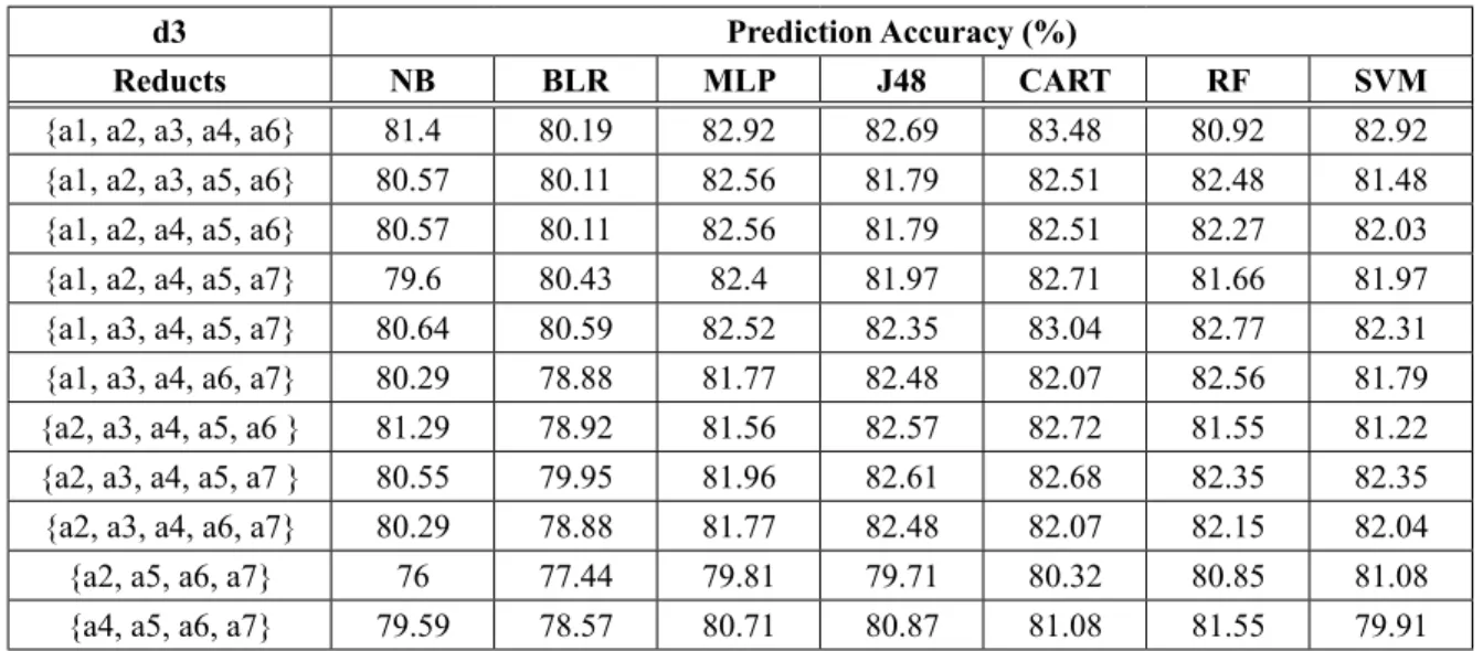
The fourteen and eleven reduct subsets gener-ated using Rosetta for the data partition d2 and d3 and the classification accuracy achieved by NB, BLR, MLP, J48, CART, RF, and SVM are presented in Tables 8 and 9.
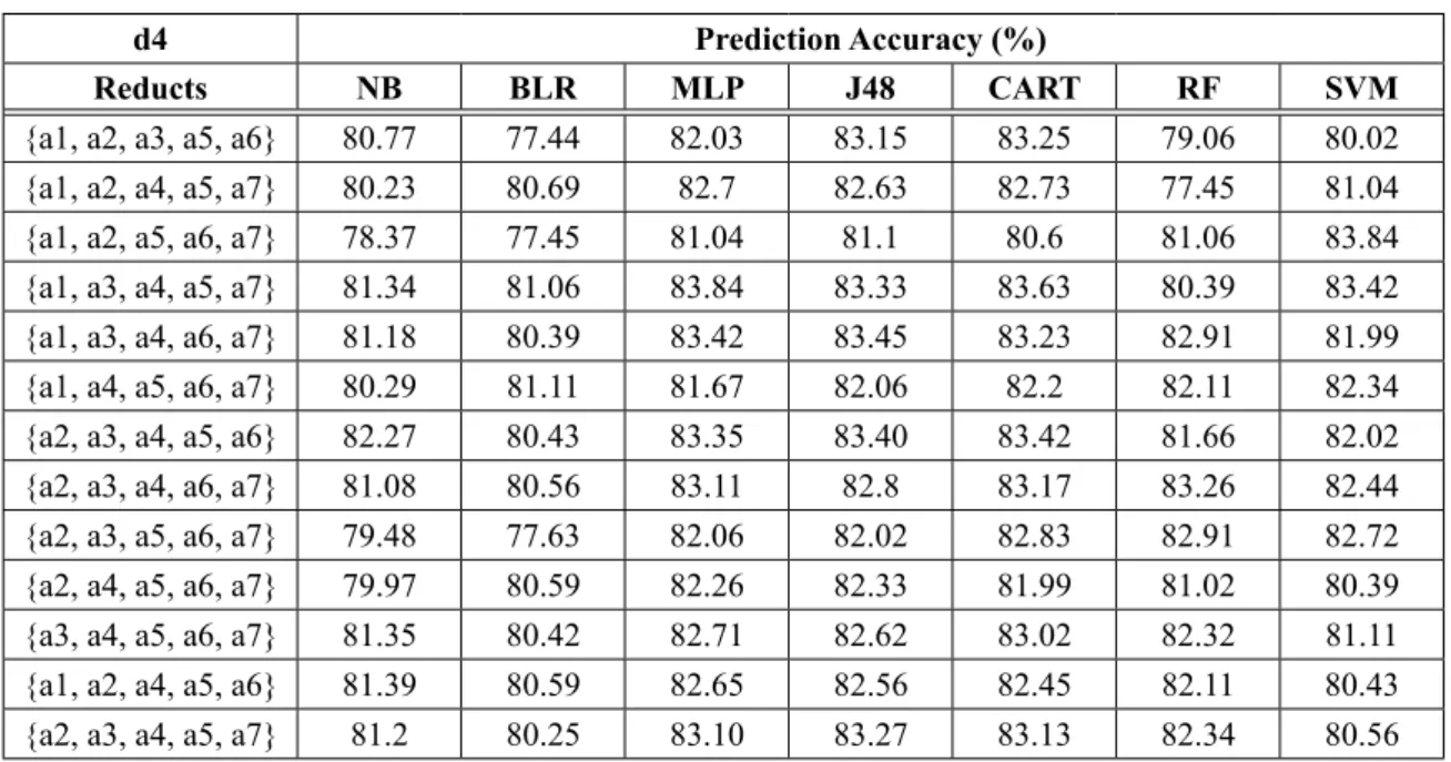
The thirteen reduct subsets generated using Ro-setta for the data partition d4 and the classifica-tion accuracy achieved by NB, BLR, MLP, J48, CART, RF, and SVM are presented in Table 10.
Table 8. Prediction accuracy of 5000 days observatory records (d2).
d2 Prediction Accuracy (%)
Reducts NB BLR MLP J48 CART RF SVM
{a1, a2, a3, a4, a7} 80.96 82.68 83.28 83.14 82.68 81.64 82.33 {a1, a2, a3, a6, a7} 82.52 80.74 84.92 83.9 84.52 81.24 81.38 {a1, a2, a4, a5, a7} 79.84 82.62 83.78 83.08 82.9 81.64 81.02 {a1, a2, a4, a6, a7} 81.64 81.38 83.5 83.32 83.78 81.24 81.38 {a1, a3, a4, a5, a7} 81.24 81.02 82.98 83.14 82.9 84.92 81.02 {a1, a3, a5, a6} 79.11 80.74 81.5 82.66 82.82 83.78 80.74 {a1, a5, a6, a7} 79.56 80.74 82.94 82.5 83.32 84.92 83.91 {a1, a2, a3, a4, a7} 80.96 82.68 83.28 83.14 82.68 83.78 81.38 {a1, a2, a3, a6, a7} 82.52 80.74 84.92 83.9 84.52 84.52 84.55 {a1, a2, a4a5, a7} 79.84 82.62 83.78 83.08 82.9 82.9 83.89 {a1, a2, a4, a6, a7} 81.64 81.38 83.5 83.32 83.78 83.78 82.62 {a1, a3, a4, a5, a7} 81.24 81.02 82.98 83.14 82.9 82.9 82.45 {a1, a3, a5, a6} 79.01 80.74 81.5 82.66 82.82 82.82 82.13 {a1, a5, a6, a7} 79.56 80.74 82.94 82.5 83.32 82.32 82.08
Table 9. Prediction accuracy of 7500 days observatory records (d3).
d3 Prediction Accuracy (%)
Reducts NB BLR MLP J48 CART RF SVM
{a1, a2, a3, a4, a6} 81.4 80.19 82.92 82.69 83.48 80.92 82.92 {a1, a2, a3, a5, a6} 80.57 80.11 82.56 81.79 82.51 82.48 81.48 {a1, a2, a4, a5, a6} 80.57 80.11 82.56 81.79 82.51 82.27 82.03 {a1, a2, a4, a5, a7} 79.6 80.43 82.4 81.97 82.71 81.66 81.97 {a1, a3, a4, a5, a7} 80.64 80.59 82.52 82.35 83.04 82.77 82.31 {a1, a3, a4, a6, a7} 80.29 78.88 81.77 82.48 82.07 82.56 81.79 {a2, a3, a4, a5, a6 } 81.29 78.92 81.56 82.57 82.72 81.55 81.22 {a2, a3, a4, a5, a7 } 80.55 79.95 81.96 82.61 82.68 82.35 82.35 {a2, a3, a4, a6, a7} 80.29 78.88 81.77 82.48 82.07 82.15 82.04 {a2, a5, a6, a7} 76 77.44 79.81 79.71 80.32 80.85 81.08 {a4, a5, a6, a7} 79.59 78.57 80.71 80.87 81.08 81.55 79.91
Table 7. Prediction accuracy of 2500 days observatory records (d1).
Prediction Accuracy of Classifiers before MFW Feature Reduction
d1 Prediction Accuracy (%)
Reducts NB BLR MLP J48 CART RF SVM
{a1, a2, a3, a4, a7} 82.68 79.68 85.12 83.8 84.28 86.4 84.56 {a4, a5, a6, a7} 86.24 77.44 89.56 89.72 89.04 86.4 89.04 {a1, a2, a5, a7} 79.64 80.44 83.6 81.52 82.08 86.4 82.08 {a1, a3, a4, a6} 86.48 79.84 88.16 87.84 88.2 79.84 88.2 {a1, a3, a5, a6} 85.68 77.44 87.04 87.08 87.36 77.44 88.16 {a1, a3, a6, a7} 88.24 77.48 89.64 88.76 89.16 77.48 89.4 {a1, a4, a5, a6} 86.4 77.92 88.4 88.04 88.16 77.92 82.56 {a1, a5, a6, a7} 86.76 77.48 89.52 89.16 89.4 89.02 88.4 {a2, a3, a4, a5} 80.28 77.4 82.24 81.36 82.56 82.24 89.52 {a2, a3, a4, a6} 87.56 78.28 88.72 87.8 88.01 82.24 82.24 {a2, a4, a5, a6} 86.4 77.4 88.62 87.87 88.54 82.24 86.81 {a2, a4, a5, a7} 81.94 78.57 85.36 85.22 84.92 77.44 85.83 {a2, a4, a6, a7} 86.81 77.44 89.18 89.44 89.39 77.44 86.35 {a2, a5, a6, a7} 85.83 77.44 89.72 89.02 89.41 78.30 79.12 {a3, a4, a5, a6} 86.35 78.3 88.45 88.28 88.62 88.4 86.81 {a3, a4, a5, a7} 79.92 80.6 81.32 80.25 81.17 89.52 85.83 {a3, a4, a6, a7} 87.37 77.8 89.34 89.66 89.48 82.24 86.35
The possible minimal reduct sets generated us-ing MFW feature selection technique for the data partition d1, d2, d3, and d4 and the classi-fication accuracy achieved by NB, BLR, MLP, J48, CART, RF, and SVM are presented in Ta-ble 11.
6.1 Comparative Analysis
The names and parameters for Weka's exhaustive search based feature selection algorithm used for comparative study is given below.
Exhaustive Search Based Feature Selection (existing method)
Run information (Weka 3.7.12)
Evaluator: weka.attributeSelection.CfsSubsetEval Search: weka.attributeSelection.ExhaustiveSearch Relation: target input
Instances: 10 000 (d4), 7500 (d3), 5000 (d3) and 2500 (d1)
Attributes: 9 (a1, a2, a3, a4, a5, a6, a7, a8, and a9) Evaluation mode: 10-fold cross-validation
6. Experimental Results and
Discussions
Minimal feature sets were assessed in terms of accuracy rate, to identify the optimal features using WEKA Software. Weka is a reliable open source machine learning and data mining tool widely adopted for a wide range of applica-tions [31]. The accuracy rate is the percentage of instances that are correctly classified by the classifier for the specified testing and training set using 10-fold cross-validation in WEKA. In 10-fold cross-validation, the model accuracy is calculated as the average error across the ten folds. The key point of this cross-validation is that it uses every possible sample for testing, and it can avoid an ill-fated split. A confusion matrix is expected as the most relevant measure for 10-fold cross-validation. The classifier per-formance for the reduct set was estimated using confusion matrix and accuracy was estimated from the confusion matrix as given in equation (3). The confusion matrix describes the actual and predicted classification done by each clas-sifier individually. The prediction accuracy of classifiers before MFW feature selection is given in Tables 7 to 10. The minimal feature
subsets projected in Table 6 is determined based on the selection criteria as represented in equation (2). The minimal and optimal feature reducts of proposed method are represented in Tables 11 and 14.
( )
R(
Tp)
Accuracy Ra Tn
Tp Tn F n e A
F t c
p
+ + + +
= (3)
[(Tp, Tn) – True positive and True negative; (Fp, Fn) – False positive and False negative] The seventeen reduct subsets generated using Rosetta for the data partition d1 and the classi-fication accuracy achieved by NB, BLR, MLP, J48, CART, RF, and SVM are presented in Ta-ble 7.
The fourteen and eleven reduct subsets gener-ated using Rosetta for the data partition d2 and d3 and the classification accuracy achieved by NB, BLR, MLP, J48, CART, RF, and SVM are presented in Tables 8 and 9.
The thirteen reduct subsets generated using Ro-setta for the data partition d4 and the classifica-tion accuracy achieved by NB, BLR, MLP, J48, CART, RF, and SVM are presented in Table 10.
Table 8. Prediction accuracy of 5000 days observatory records (d2).
d2 Prediction Accuracy (%)
Reducts NB BLR MLP J48 CART RF SVM
{a1, a2, a3, a4, a7} 80.96 82.68 83.28 83.14 82.68 81.64 82.33 {a1, a2, a3, a6, a7} 82.52 80.74 84.92 83.9 84.52 81.24 81.38 {a1, a2, a4, a5, a7} 79.84 82.62 83.78 83.08 82.9 81.64 81.02 {a1, a2, a4, a6, a7} 81.64 81.38 83.5 83.32 83.78 81.24 81.38 {a1, a3, a4, a5, a7} 81.24 81.02 82.98 83.14 82.9 84.92 81.02 {a1, a3, a5, a6} 79.11 80.74 81.5 82.66 82.82 83.78 80.74 {a1, a5, a6, a7} 79.56 80.74 82.94 82.5 83.32 84.92 83.91 {a1, a2, a3, a4, a7} 80.96 82.68 83.28 83.14 82.68 83.78 81.38 {a1, a2, a3, a6, a7} 82.52 80.74 84.92 83.9 84.52 84.52 84.55 {a1, a2, a4a5, a7} 79.84 82.62 83.78 83.08 82.9 82.9 83.89 {a1, a2, a4, a6, a7} 81.64 81.38 83.5 83.32 83.78 83.78 82.62 {a1, a3, a4, a5, a7} 81.24 81.02 82.98 83.14 82.9 82.9 82.45 {a1, a3, a5, a6} 79.01 80.74 81.5 82.66 82.82 82.82 82.13 {a1, a5, a6, a7} 79.56 80.74 82.94 82.5 83.32 82.32 82.08
Table 9. Prediction accuracy of 7500 days observatory records (d3).
d3 Prediction Accuracy (%)
Reducts NB BLR MLP J48 CART RF SVM
{a1, a2, a3, a4, a6} 81.4 80.19 82.92 82.69 83.48 80.92 82.92 {a1, a2, a3, a5, a6} 80.57 80.11 82.56 81.79 82.51 82.48 81.48 {a1, a2, a4, a5, a6} 80.57 80.11 82.56 81.79 82.51 82.27 82.03 {a1, a2, a4, a5, a7} 79.6 80.43 82.4 81.97 82.71 81.66 81.97 {a1, a3, a4, a5, a7} 80.64 80.59 82.52 82.35 83.04 82.77 82.31 {a1, a3, a4, a6, a7} 80.29 78.88 81.77 82.48 82.07 82.56 81.79 {a2, a3, a4, a5, a6 } 81.29 78.92 81.56 82.57 82.72 81.55 81.22 {a2, a3, a4, a5, a7 } 80.55 79.95 81.96 82.61 82.68 82.35 82.35 {a2, a3, a4, a6, a7} 80.29 78.88 81.77 82.48 82.07 82.15 82.04 {a2, a5, a6, a7} 76 77.44 79.81 79.71 80.32 80.85 81.08 {a4, a5, a6, a7} 79.59 78.57 80.71 80.87 81.08 81.55 79.91
Table 7. Prediction accuracy of 2500 days observatory records (d1).
Prediction Accuracy of Classifiers before MFW Feature Reduction
d1 Prediction Accuracy (%)
Reducts NB BLR MLP J48 CART RF SVM
{a1, a2, a3, a4, a7} 82.68 79.68 85.12 83.8 84.28 86.4 84.56 {a4, a5, a6, a7} 86.24 77.44 89.56 89.72 89.04 86.4 89.04 {a1, a2, a5, a7} 79.64 80.44 83.6 81.52 82.08 86.4 82.08 {a1, a3, a4, a6} 86.48 79.84 88.16 87.84 88.2 79.84 88.2 {a1, a3, a5, a6} 85.68 77.44 87.04 87.08 87.36 77.44 88.16 {a1, a3, a6, a7} 88.24 77.48 89.64 88.76 89.16 77.48 89.4 {a1, a4, a5, a6} 86.4 77.92 88.4 88.04 88.16 77.92 82.56 {a1, a5, a6, a7} 86.76 77.48 89.52 89.16 89.4 89.02 88.4 {a2, a3, a4, a5} 80.28 77.4 82.24 81.36 82.56 82.24 89.52 {a2, a3, a4, a6} 87.56 78.28 88.72 87.8 88.01 82.24 82.24 {a2, a4, a5, a6} 86.4 77.4 88.62 87.87 88.54 82.24 86.81 {a2, a4, a5, a7} 81.94 78.57 85.36 85.22 84.92 77.44 85.83 {a2, a4, a6, a7} 86.81 77.44 89.18 89.44 89.39 77.44 86.35 {a2, a5, a6, a7} 85.83 77.44 89.72 89.02 89.41 78.30 79.12 {a3, a4, a5, a6} 86.35 78.3 88.45 88.28 88.62 88.4 86.81 {a3, a4, a5, a7} 79.92 80.6 81.32 80.25 81.17 89.52 85.83 {a3, a4, a6, a7} 87.37 77.8 89.34 89.66 89.48 82.24 86.35
The possible minimal reduct sets generated us-ing MFW feature selection technique for the data partition d1, d2, d3, and d4 and the classi-fication accuracy achieved by NB, BLR, MLP, J48, CART, RF, and SVM are presented in Ta-ble 11.
6.1 Comparative Analysis
The names and parameters for Weka's exhaustive search based feature selection algorithm used for comparative study is given below.
Exhaustive Search Based Feature Selection (existing method)
Run information (Weka 3.7.12)
Evaluator: weka.attributeSelection.CfsSubsetEval Search: weka.attributeSelection.ExhaustiveSearch Relation: target input
Instances: 10 000 (d4), 7500 (d3), 5000 (d3) and 2500 (d1)
Attributes: 9 (a1, a2, a3, a4, a5, a6, a7, a8, and a9) Evaluation mode: 10-fold cross-validation
Table 10. Prediction accuracy of 10 000 days observatory records (d4).
d4 Prediction Accuracy (%)
Reducts NB BLR MLP J48 CART RF SVM
{a1, a2, a3, a5, a6} 80.77 77.44 82.03 83.15 83.25 79.06 80.02 {a1, a2, a4, a5, a7} 80.23 80.69 82.7 82.63 82.73 77.45 81.04 {a1, a2, a5, a6, a7} 78.37 77.45 81.04 81.1 80.6 81.06 83.84 {a1, a3, a4, a5, a7} 81.34 81.06 83.84 83.33 83.63 80.39 83.42 {a1, a3, a4, a6, a7} 81.18 80.39 83.42 83.45 83.23 82.91 81.99 {a1, a4, a5, a6, a7} 80.29 81.11 81.67 82.06 82.2 82.11 82.34 {a2, a3, a4, a5, a6} 82.27 80.43 83.35 83.40 83.42 81.66 82.02 {a2, a3, a4, a6, a7} 81.08 80.56 83.11 82.8 83.17 83.26 82.44 {a2, a3, a5, a6, a7} 79.48 77.63 82.06 82.02 82.83 82.91 82.72 {a2, a4, a5, a6, a7} 79.97 80.59 82.26 82.33 81.99 81.02 80.39 {a3, a4, a5, a6, a7} 81.35 80.42 82.71 82.62 83.02 82.32 81.11 {a1, a2, a4, a5, a6} 81.39 80.59 82.65 82.56 82.45 82.11 80.43 {a2, a3, a4, a5, a7} 81.2 80.25 83.10 83.27 83.13 82.34 80.56
Table 11. Minimal feature reduct sets Prediction Accuracy.
Prediction Accuracy of Classifiers After MFW Feature Reduction
Dataset Minimal Reducts NB BLR MLP J48 CART RF SVM
d1 {a3, a4, a5, a6, a7} 79.92 80.6 81.32 80.25 81.17 81.72 81.07 {a4, a5, a6, a7} 86.24 77.44 89.56 89.72 89.04 83.53 82.65
d2
{a1, a2, a4, a5, a7} 79.84 82.62 83.78 83.08 82.90 82.11 81.02 {a1, a2, a4, a6, a7} 81.64 81.38 83.5 83.32 83.78 83.45 81.38 {a1, a2, a3, a4, a7} 80.96 82.68 83.28 83.14 82.68 83.07 82.33 {a1, a3, a4, a5, a7} 81.24 81.02 82.98 83.14 82.90 81.57 82.45
d3
{a2, a4, a5, a6, a7} 81.29 78.92 81.56 82.57 82.72 81.72 82.03 {a2, a3, a4, a6, a7} 80.29 78.88 81.77 82.48 82.07 82.32 82.04 {a2, a3, a4, a5, a6} 81.29 78.92 81.56 82.57 82.72 82.21 82.35
d4
{a2, a4, a5, a6, a7} 79.17 80.59 82.26 82.33 81.99 82.32 80.39 {a2, a3, a4, a5, a6} 82.27 80.43 83.35 83.4 83.42 83.01 82.02 {a2, a3, a5, a6, a7} 79.48 77.63 82.06 82.02 82.83 81.79 82.72
An existing exhaustive search based attribute selection approach was used for comparison and validation of the proposed MFW feature reduction model. The existing approach identi-fied {a3, a4, a7, a8}, {a2, a3, a4, a7, a8}, {a2, a4, a6, a7, a8}, and {a2, a4, a6} feature subsets for the input d4, d3, d2, and d1 as projected in Table 13 using WEKA (http://www.cs.waikato. ac.nz/ml/weka).
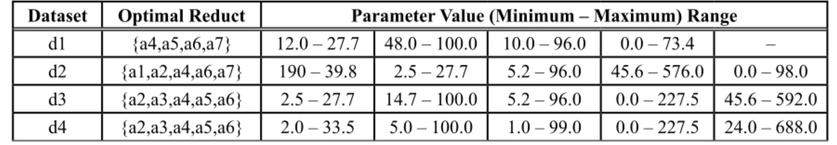
The optimal reduct set and the achieved pre-diction accuracy is shown in Table 14. The weather parameter values of optimal reduct sets
for classifiers in achieving classification results are shown in Table 15.
The accuracy of subsets generated using the existing exhaustive search and the proposed MFW feature reduction approach have been thoroughly examined.
For the above investigational results presented in Table 7 to Table 14 the clasisfiers were set with default parameter values. Some of the parameters values for classifiers in achieving classification results are presented in Table 16.
The rainfall prediction accuracy of proposed model when compared with some popular ex-isting models as in Table 17 reveal that the proposed technique outperformed the existing approaches.
The classifiers trained using the feature sub-sets generated using MFW reduction technique have improved the prediction accuracy. CART
and J48 classifier obtained 83.42%, 83.72%, 83.78% and 89.72% prediction accuracy for dataset d4, d3, d2 and d1 respectively. MFW feature selection approach is capable of find-ing some set of suitable subsets rather than just finding one subset after the attribute evaluation. From the possible combinations one can identify the indispensable attribute using the 'core'
prop-Table 12. Feature subsets generated using existing exhaustive search approach.
Attributes Number of folds (%) attribute
d4 d3 d2 d1
a1 (Max) 0 0 0 0
a2 (Min) 0 100 100 100
a3 (RH1) 50 100 40 0
a4 (RH2) 100 100 100 100
a5 (WS) 0 0 0 0
a6 (SR) 0 0 100 100
a7 (SS) 100 100 100 20
a8 (EVP) 100 100 100 0
Feature Subset {a3,a4,a7,a8} {a2,a3,a4,a7,a8} {a2,a4,a6,a7,a8} {a2,a4,a6}
Table 13. Prediction accuracy (%) of reducts based on existing exhaustive search.
Dataset Reducts NB BLR MLP J48 CART RF SVM
d1 {a2,a4,a6} 86.22 81.56 87.09 88.12 86.53 84.34 88.07 d2 {a2,a4,a6,a7,a8} 81.34 7921 82.5 79.04 81.08 79.67 81.07 d3 {a2,a3,a4,a7,a8} 79.98 80.33 81.85 82.33 82.12 78.55 80.01 d4 {a3,a4,a7,a8} 81.23 80.07 79.05 81.21 81.07 79.04 79.71
Table 14. Prediction accuracy (%) of optimal reducts based on MFW feature selection.
Dataset Optimal Reducts NB BLR MLP J48 CART RF SVM
d1 {a4,a5,a6,a7} 86.24 77.44 89.56 89.72 89.04 86.4 89.04 d2 {a1,a2,a4,a6,a7} 81.64 81.38 83.5 83.32 83.78 81.24 81.38 d3 {a2,a3,a4,a5,a6} 81.29 78.92 81.56 82.57 82.72 81.55 81.22 d4 {a2,a3,a4,a5,a6} 82.27 80.43 83.35 83.4 83.42 81.66 82.02
Table 15. Parameter values of optimal reduct for achieving better prediction accuracy.
Dataset Optimal Reduct Parameter Value (Minimum – Maximum) Range
Table 10. Prediction accuracy of 10 000 days observatory records (d4).
d4 Prediction Accuracy (%)
Reducts NB BLR MLP J48 CART RF SVM
{a1, a2, a3, a5, a6} 80.77 77.44 82.03 83.15 83.25 79.06 80.02 {a1, a2, a4, a5, a7} 80.23 80.69 82.7 82.63 82.73 77.45 81.04 {a1, a2, a5, a6, a7} 78.37 77.45 81.04 81.1 80.6 81.06 83.84 {a1, a3, a4, a5, a7} 81.34 81.06 83.84 83.33 83.63 80.39 83.42 {a1, a3, a4, a6, a7} 81.18 80.39 83.42 83.45 83.23 82.91 81.99 {a1, a4, a5, a6, a7} 80.29 81.11 81.67 82.06 82.2 82.11 82.34 {a2, a3, a4, a5, a6} 82.27 80.43 83.35 83.40 83.42 81.66 82.02 {a2, a3, a4, a6, a7} 81.08 80.56 83.11 82.8 83.17 83.26 82.44 {a2, a3, a5, a6, a7} 79.48 77.63 82.06 82.02 82.83 82.91 82.72 {a2, a4, a5, a6, a7} 79.97 80.59 82.26 82.33 81.99 81.02 80.39 {a3, a4, a5, a6, a7} 81.35 80.42 82.71 82.62 83.02 82.32 81.11 {a1, a2, a4, a5, a6} 81.39 80.59 82.65 82.56 82.45 82.11 80.43 {a2, a3, a4, a5, a7} 81.2 80.25 83.10 83.27 83.13 82.34 80.56
Table 11. Minimal feature reduct sets Prediction Accuracy.
Prediction Accuracy of Classifiers After MFW Feature Reduction
Dataset Minimal Reducts NB BLR MLP J48 CART RF SVM
d1 {a3, a4, a5, a6, a7} 79.92 80.6 81.32 80.25 81.17 81.72 81.07 {a4, a5, a6, a7} 86.24 77.44 89.56 89.72 89.04 83.53 82.65
d2
{a1, a2, a4, a5, a7} 79.84 82.62 83.78 83.08 82.90 82.11 81.02 {a1, a2, a4, a6, a7} 81.64 81.38 83.5 83.32 83.78 83.45 81.38 {a1, a2, a3, a4, a7} 80.96 82.68 83.28 83.14 82.68 83.07 82.33 {a1, a3, a4, a5, a7} 81.24 81.02 82.98 83.14 82.90 81.57 82.45
d3
{a2, a4, a5, a6, a7} 81.29 78.92 81.56 82.57 82.72 81.72 82.03 {a2, a3, a4, a6, a7} 80.29 78.88 81.77 82.48 82.07 82.32 82.04 {a2, a3, a4, a5, a6} 81.29 78.92 81.56 82.57 82.72 82.21 82.35
d4
{a2, a4, a5, a6, a7} 79.17 80.59 82.26 82.33 81.99 82.32 80.39 {a2, a3, a4, a5, a6} 82.27 80.43 83.35 83.4 83.42 83.01 82.02 {a2, a3, a5, a6, a7} 79.48 77.63 82.06 82.02 82.83 81.79 82.72
An existing exhaustive search based attribute selection approach was used for comparison and validation of the proposed MFW feature reduction model. The existing approach identi-fied {a3, a4, a7, a8}, {a2, a3, a4, a7, a8}, {a2, a4, a6, a7, a8}, and {a2, a4, a6} feature subsets for the input d4, d3, d2, and d1 as projected in Table 13 using WEKA (http://www.cs.waikato. ac.nz/ml/weka).
The optimal reduct set and the achieved pre-diction accuracy is shown in Table 14. The weather parameter values of optimal reduct sets
for classifiers in achieving classification results are shown in Table 15.
The accuracy of subsets generated using the existing exhaustive search and the proposed MFW feature reduction approach have been thoroughly examined.
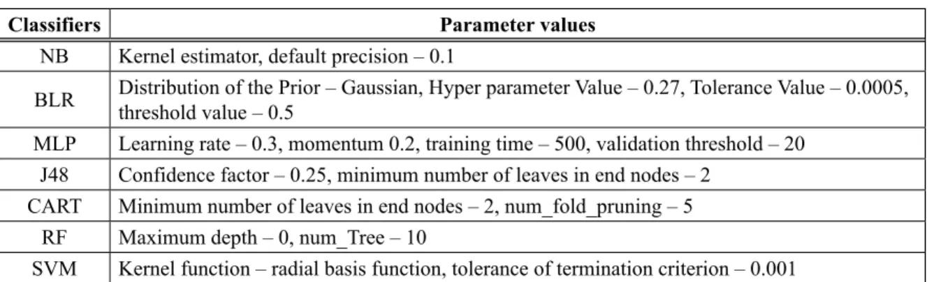
For the above investigational results presented in Table 7 to Table 14 the clasisfiers were set with default parameter values. Some of the parameters values for classifiers in achieving classification results are presented in Table 16.
The rainfall prediction accuracy of proposed model when compared with some popular ex-isting models as in Table 17 reveal that the proposed technique outperformed the existing approaches.
The classifiers trained using the feature sub-sets generated using MFW reduction technique have improved the prediction accuracy. CART
and J48 classifier obtained 83.42%, 83.72%, 83.78% and 89.72% prediction accuracy for dataset d4, d3, d2 and d1 respectively. MFW feature selection approach is capable of find-ing some set of suitable subsets rather than just finding one subset after the attribute evaluation. From the possible combinations one can identify the indispensable attribute using the 'core'
prop-Table 12. Feature subsets generated using existing exhaustive search approach.
Attributes Number of folds (%) attribute
d4 d3 d2 d1
a1 (Max) 0 0 0 0
a2 (Min) 0 100 100 100
a3 (RH1) 50 100 40 0
a4 (RH2) 100 100 100 100
a5 (WS) 0 0 0 0
a6 (SR) 0 0 100 100
a7 (SS) 100 100 100 20
a8 (EVP) 100 100 100 0
Feature Subset {a3,a4,a7,a8} {a2,a3,a4,a7,a8} {a2,a4,a6,a7,a8} {a2,a4,a6}
Table 13. Prediction accuracy (%) of reducts based on existing exhaustive search.
Dataset Reducts NB BLR MLP J48 CART RF SVM
d1 {a2,a4,a6} 86.22 81.56 87.09 88.12 86.53 84.34 88.07 d2 {a2,a4,a6,a7,a8} 81.34 7921 82.5 79.04 81.08 79.67 81.07 d3 {a2,a3,a4,a7,a8} 79.98 80.33 81.85 82.33 82.12 78.55 80.01 d4 {a3,a4,a7,a8} 81.23 80.07 79.05 81.21 81.07 79.04 79.71
Table 14. Prediction accuracy (%) of optimal reducts based on MFW feature selection.
Dataset Optimal Reducts NB BLR MLP J48 CART RF SVM
d1 {a4,a5,a6,a7} 86.24 77.44 89.56 89.72 89.04 86.4 89.04 d2 {a1,a2,a4,a6,a7} 81.64 81.38 83.5 83.32 83.78 81.24 81.38 d3 {a2,a3,a4,a5,a6} 81.29 78.92 81.56 82.57 82.72 81.55 81.22 d4 {a2,a3,a4,a5,a6} 82.27 80.43 83.35 83.4 83.42 81.66 82.02
Table 15. Parameter values of optimal reduct for achieving better prediction accuracy.
Dataset Optimal Reduct Parameter Value (Minimum – Maximum) Range
References
[1] J. H. Seo and Y. H. Kim, “A survey on rainfall forecast algorithms based on machine learning technique”, in Proceedings of the KIIS Fall Con-ference, Korea, 2011.
[2] G. E. Afandi et al., “Heavy rainfall simulation over Sinai Peninsula using the weather research and forecasting model”, International Journal of Atmospheric Sciences, p. 11, 2013.
[3] H. D. LEE et al., “Feature selection for heavy rain prediction using genetic algorithms”, in Interna-tional Symposium on Advanced Intelligent Sys-tems, IEEE, Kobe, Japan, November 2012. [4] Z. Pawlak et al., “Rough sets”, Communications
of the ACM, vol. 38, no. 11, pp. 89–95, 1995. http://dx.doi.org/10.1145/219717.219791
[5] Z. Pawlak and R. Slowinski, “Rough set approach to multi-attribute decision analysis”, European Journal of Operational Research, vol. 72, no. 3, pp. 443–459, 1994.
http://dx.doi.org/10.1016/0377-2217(94)90415-4 [6] Z. Pawlak and R. Slowinski, “Decision analysis
using rough sets”, International Transactions on Operational Research, vol. 1, pp. 107–114, 1994. http://dx.doi.org/10.1016/0969-6016(94)90050-7 [7] Z. Pawlak, “Rough sets”, International Journal
of Information and Computer Sciences, vol. 11, no. 5, pp. 341–356, 1982.
http://dx.doi.org/10.1007/BF01001956
[8] Z. Pawlak, “Rough sets and its applications”,
Journal of Telecommunications and Information Technology, pp. 7–10, 2002.
[9] Z. Pawlak and A. Skowron, “Rough sets: some extensions”, Information Sciences, vol. 177, pp. 28–40, 2007.
http://dx.doi.org/10.1016/j.ins.2006.06.007 [10] Q. Shen and R. Jensen, “Rough sets their
exten-sions and applications”, International Journal of Automation and Computing, vol. 4, no. 1, pp. 100–106, 2007.
http://dx.doi.org/10.1007/s11633-007-0217-y [11] A. Ohrn, Rosetta technical reference manual,
De-partment of Computer and Information Science, Norwegian University of Science and Technol-ogy, Trondheim, Norwa, 2001.
[12] J. N. K. Liu et al., “An improved Naive Bayesian classifier technique coupled with a novel input solution method”, IEEE Transactions on Systems, Man and Cybernetics, vol. 31, no. 2, pp. 249–256, 2001.
http://dx.doi.org/10.1109/5326.941848
Table 16. Classifier (default) parameter value.
Classifiers Parameter values
NB Kernel estimator, default precision – 0.1
BLR Distribution of the Prior – Gaussian, Hyper parameter Value – 0.27, Tolerance Value – 0.0005, threshold value – 0.5 MLP Learning rate – 0.3, momentum 0.2, training time – 500, validation threshold – 20
J48 Confidence factor – 0.25, minimum number of leaves in end nodes – 2 CART Minimum number of leaves in end nodes – 2, num_fold_pruning – 5
RF Maximum depth – 0, num_Tree – 10
SVM Kernel function – radial basis function, tolerance of termination criterion – 0.001
Table 17. Rainfall prediction accuracy (%) of existing approaches.
Literature Meteorological Data Registered (Region) Technique Prediction Accuracy
[32] Cuddalore in East Coast of India. Temperature, dew point, wind speed, visibility Predictive a priori Algorithm, K*
Algorithm 75.72%
[33]
Accuweather.com of Indian Meteorological Department. (1998 to 2012) 9 Yrs. Humidity,
temperature, pressure, wind speed, and dew point
Supervised Learning in Quest decision tree using gain ratio
Decision Tree
77.78%
[34] temperature, maximum temperature, pressure, Assam (2007 – 2012) 6 Yrs. Minimum wind direction, relative humidity
Multiple Linear
Regression 63%
[35] Dongtai – coastal city of East China. Pressure, temperature, extreme maximum temperature, relative humidity
Tree Augmented Naïve Bayes model Naïve
Bayes 62.5% 50%
[13] E. A. Alikhashashneh and Q. A. Al-Radaideh, “Evaluation of discernibility matrix based reduct computation techniques”, in International Con-ference on Computer Science and Software En-gineering, 2013.
http://dx.doi.org/10.1109/csit.2013.6588762 [14] L. Ju, “Attribution reduction algorithm based on
improved binary dicernibility matrix”, in Inter-national Conference on Computer and Electrical Engineering, Chengdu, Sichuan, China, 2010. [15] T. Kanik, “Hepatitis disease diagnosis using
rough set modification of the pre-processing al-gorithm”, in Proceedings in Information and Communication Technologies International Con-ference, Atlanta, Georgia, 2012.
[16] W. Hao and X. Zhang, A simplified discernibility matrix of the attribute selection method, Interna-tional conference on Information Management, (2010).
[17] Y. Y. Yao and Y. Zhao, “Discernibility matrix sim-plification for constructing attribute reducts”, In-formation Sciences, vol. 179, no. 5, pp. 867–882, 2009.
http://dx.doi.org/10.1016/j.ins.2008.11.020 [18] W. C. Hong, “Rainfall forecasting by
technolog-ical machine learning models”, Applied Mathe-matics and Computation, vol. 1, pp. 41–57, 2008. http://dx.doi.org/10.1016/j.amc.2007.10.046 [19] J. Dai and Q. Xu, “Attribute selection based on
in-formation gain ratio in fuzzy rough set theory with application to tumour classification”, Applied Soft Computing, vol. 13, pp. 211–221, 2013.
http://dx.doi.org/10.1016/j.asoc.2012.07.029 [20] Y. Huang and S. Chen, “An algorithm of attribute
selection based on rough sets”, Physics procedia, pp. 2025–2029, 2013.
[21] N. Suguna and G. Thanushkodi, “An indepen-dent rough set approach hybrid with artificial bee colony algorithm for dimensionality reduction”,
American Journal of Applied Sciences, vol. 8, no. 3, pp. 261–266, 2011.
http://dx.doi.org/10.3844/ajassp.2011.261.266 [22] T. Qablan and S. A. Shuqeir, “A reduct
computa-tion approach based on ant colony optimizacomputa-tion”,
Basic Science and Engineering, vol. 21, no. 1, pp. 29–40, 2012.
[23] W. Wei et al., “A comparative study of rough sets for hybrid data”, Information Sciences, vol. 190, pp. 1–16, 2012.
http://dx.doi.org/10.1016/j.ins.2011.12.006 [24] S. Greco et al., “Rough set theory for
multi-crite-ria decision analysis”, European Journal of Oper-ational Research, pp. 1–47, 2001.
http://dx.doi.org/10.1016/S0377-2217(00)00167-3 erty of rough set from equation (1) as defined
by Pawlak. The experimental study of learning algorithms before and after using MFW feature selection revealed that the performance of the learning algorithms has been improved when trained using optimal feature set.
7. Conclusion
The novel MFW feature reduction has identified relative humidity2 (a4) and solar radiation (a6) as indispensable or core parameters for rain-fall prediction according to RST. Experimental study and evaluations conducted using the op-timal subset on classification algorithms indi-cated that the accuracy rate of the classification models has improved after the feature selection using MFW feature selection approach. Exper-imental results conclude that this investigation