Robust H1 Control of a Doubly Fed Asynchronous Machine

Robust H

∞

Control of a Doubly Fed Asynchronous Machine

Gherbi Sofiane

Department of electrical engineering, Faculty of Science of the engineer 20 August 1956 University, Skikda, Algeria

E-mail: [email protected] Yahmedi Said

Department of electronic, Faculty of Science of the engineer Badji Mokhtar University, Annaba, Algeria

E-mail: [email protected] Sedraoui Moussa

Department of electronics, Faculty of Science of the engineer Constantine University, road of AIN EL BEY Constantine, Algeria E-mail : [email protected]

Keywords:doubly fed asynchronous machine, robust control,H_control, LMI’s

Received:April 25, 2008

The doubly fed asynchronous machine is among the most used electrical machines due to its low cost, simplicity of construction and maintenance [1]. In this paper, we present a method to synthesize a robust controller of doubly fed asynchronous machine which is the main component of the wind turbine system (actually the most used model [2]), indeed: there is different challenges in the control of the wind energy systems and we have to take in a count a several parameters that perturb the system as: the wind speed variation, the consumption variation of the electricity energy and the kind of the power consumed (active or reactive) ...etc.. The method proposed is based on the Hcontrol problem with the linear

matrix inequalities (LMI’s) solution: Gahinet-Akparian [3], the results show the stability and the performance robustness of the system in spite of the perturbations mentioned before.

Povzetek: Opisana je metoda upravljanja motorja vetrnih turbin.

1 Introduction

From all the renewable energy electricity production systems, the wind turbine systems are the most used specially the doubly fed asynchronous machine based systems, the control of theses systems is particularly difficult because all of the uncertainties introduced such as: the wind speed variations, the electrical energy consumption variation, the system parameters variations, in this paper we focus on the robust control (H_controller design method) of the doubly fed

asynchronous machine which is the most used in the wind turbine system due to its low cost, simplicity of construction and maintenance [1].

This paper is organised as follow:

Section 2 presents the wind turbine system equipped with the doubly fed asynchronous machine and then the mathematical electrical equations from what the system is modelled (in the state space form) are given.

The section 3 presents the H robust controller design

method with the LMI’s solution used to control our system.

The section 4 presents a numerical application and results in both the frequency and time plan are presented And finally a conclusion is given in section 5.

2 System presentation and

modelling

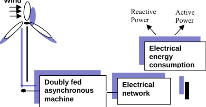
The following figure represents the wind turbine system

The system use the wind power to drag the double fed asynchronous machine who acts as a generator, the output power produced must have the same high quality when it enters the electrical network, i.e.: 220 volts amplitude and 60 Hz frequency and the harmonics held

Active Power

Doubly fed asynchronous machine Wind

Electrical network

Electrical energy consumption

Reactive Power

to a low level in spite of wind speed changes and electrical energy consumption in active or reactive power form. References [4], [5], [6] describe detailed models of wind turbines for simulations, we use the model equipped with the doubly fed induction generators (asynchronous machine) (for more details see [7]), the system electrical equations are given in

 

d, frame orientation, then the stator voltage q

differential equations are:

qs s ds ds s ds w dt d I R

V  .     (1)

ds s qs qs s qs w dt d I R

V  .     (2) The rotor voltage differential equations are:

qr r dr dr r dr w dt d I R

V  .     (3)

dr r qr qr r qr w dt d I R

V  .     (4) The stator flux vectors equations are:

dr ds s

ds L .I M.I

 (5)

qr qs s

qs L .I M.I

 (6) The rotor flux vectors equations:

ds dr r

dr L .I M.I

 (7)

qs qr

r

qr L .I M.I

 (8) The electromagnetic couple flux equation :

) . .

(

. _{ds qr qs dr}

s

em I I

L M p

C    (9)

The electromagnetic couple mecanic equation : 

  

 f.

dt d J C

C_{em r} (10)

With:

qs ds V

V , : Statoric voltage vector components in ‘d’

and ‘q’ axes respectively. qr

dr V

V , : Rotoric voltage vector components in ‘d’

and ‘q’ axes respectively. qs

ds I

I , : Statoric current vector components in ‘d’

and ‘q’ axes respectively. qr

dr I

I , : Rotoric current vector components in ‘d’

and ‘q’ axes respectively. qs

ds 

 , : Statoric flux vector components in ‘d’

and ‘q’ axes respectively. qr

dr 

 , : Rotoric flux vector components in ‘d’

and ‘q’ axes respectively. r

s R

R , : Stator and rotor resistances (of one phase) respectively.

r s L

L , : Stator and rotor cyclic inductances respectively.

r s w

w , : Statoric and rotoric current pulsations respectively.

M : Cyclic mutual inductance.

p : Number of pair of the machine poles.

r

C : Resistant torque.

f : Viscous rubbing coefficient.

J : Inertia moment.

2.1

State space model

In order to apply the robust controller design method, we have to put the system model in the state space from; we consider the rotoric voltage

V

dr

,

V

qras the inputs

and the statoric voltage

V

_ds

,

V

_qs as the outputs, i.e. we have to design a controller who acts on the rotoric voltages to keep the output statoric voltages at

volts

220 and50Hzfrequency in spite of the electric

network perturbations (demand variations … etc) and the wind speed variations (see figure.2).

Figure 2: A Doubly fed wind turbine system control configuration

Where: u,yand eare the rotoric voltage vector

(control vector), statoric output voltage vector and the error signal between the input reference and the output system respectively.K,Gare the controller and the

wind turbine system respectively.

R

: is the statoric voltage references vector and perturbations are the

electric energy demand variations, wind speed variations …etc.

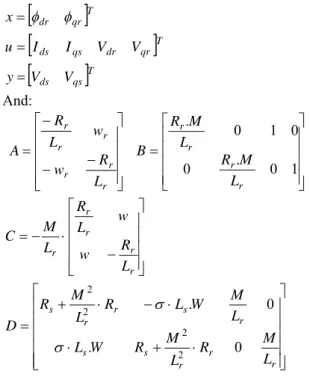
Let us consider





T qr dr

x   as a state vector, and





T

qs ds qs

ds I V V I

u as the command vector, the

stator flux vector is oriented in d axis of Parks reference frame then : _qs 0 and Ids,Iqsare considered constant in the steady state i.e.: I_ds I_qs 0.

We use the folowing doubly fed asynchronous machine parameters:

 5

s

R ;R_r 1.0113 ;M 0.1346H H

L_s0.3409 ;L_r0.605H ;w_r 146.6Hz ; Hz

w_s 250

Let wwswr and

r s L L M   1 2

 .

The state space (11) can be obtained by the combining of the equations (1) to (8) as follow:

           u D x C y u B x A x (11) Where: ons perturbati G

R e u y





T qr dr

x  





T

qr dr qs

ds I V V

I u





T

qs ds V V y And:                 r r r r r r L R w w L R A              1 0 . 0 0 1 0 . r r r r L M R L M R B                 r r r r r L R w w L R L M C                       r r r s s r s r r s L M R L M R W L L M W L R L M R D 0 . 0 . 2 2 2 2  

3 The

H

∞

controller design method

It is necessary to recall the basics of a control loop (figure.3). With G’_{: the perturbed system.}

Figure 3: The control loop with the output multiplicative uncertainties

The multiplicative uncertainties at the process output which include all the perturbations that act in the system are then : _{ (} '_{ ).} 1

G G G

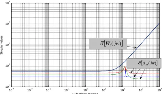
m , with GG(Im) : is

the perturbed system, figure.4 show the singular values plot at the frequency plan of



_m, we can see that the uncertainties are smaller at low frequencies and grow at the medium and high frequencies, this mean a strong perturbation at high frequencies (the transient phase), we also note a pick at:





260

rad

/

s

, this is due to the fact that the system is highly coupled at this pulsation.

We can bound the system uncertainties by the following weighting matrix function:

                 ) 0001 . 0 1 ( ) 1 02 . 0 ( 55 . 0 0 0 ) 0001 . 0 1 ( ) 1 02 . 0 ( 55 . 0 ) ( jw jw jw jw jw

W_t (12)

The figure.5 show that the singular values of )

(jw

W_t bounds the maximum singular values of the

uncertainties in the entire frequency plan. The robust stability condition [11] is then:





T

   

jw Wt jw



1 (13) Or:





T

 

jw







W_t

 

jw



1 (14)

Where:



is the maximum singular value and T

 

jw is

the nominal closed loop transfer matrix defined by:

 

_

   

_{ }



_

   

_



1

jw K jw G I jw K jw G jw

T (15)

The equations (13) allow us to guaranty the stability robustness, in other hand we most guaranty satisfying performances (no overshoot, time response …etc) in the closed loop (performances robustness), this can by done by the performance robustness condition [8]:

 

 



S

jw



W

_p

jw





1



(16) Or:

 





_



 



1

jw

W

jw

S



_p



(17) Where:

 

jw

S is the sensitivity matrix given by:

 

_



_

   

_



1

jw K jw G I jw

S (18)

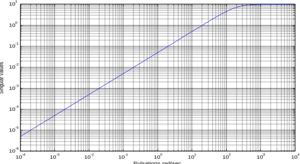
) (jw

W_P is a weighting matrix function designed to meet

the performance specifications desired in the frequency plan, we choose the following matrix function:

               jw jw jw jw jw Wp 05 . 0 ) 1 005 . 0 ( 0 0 05 . 0 ) 1 005 . 0 ( )

( (19)

The figure.6 represent the singular values of W_P

 

jw in

the frequency plan, one notice that the specifications on the performances are bigger in low frequencies (integrator frequency behaviour), and this guaranty no static error.

Then the standard problem of H∞ Control theory is then:

   

 



 

_



jw

W

jw

S

jw

W

jw

p g stabili K t sin

T

min

(20)

i.e.: to find a stabilising controllerKthat minimise the norm (20).

With: _ is The Hinfinity norm.

∆m

K G y

G’

_

4 Application

The minimisation problem (20) is solved by using two Riccati equations [9] or with the linear matrix inequalities approach. For our system, we use the linear matrix inequalities solution (for more details see [10]). The solution (controller) can be obtained via the Matlab instruction hinflmi available at ‘LMI Toolbox’ of

Matlab®_{Math works Inc [11].}

The figure 7 and the figure 8 show the satisfaction of the stability and performances robustness conditions (14) and (17).

The figure.9 show the step responses step responses of the closed loop controlled nominal system with:



0₁



0 1

_

_  

 V_{ds ref} V_{qs ref}

R respectively.

The Outputs Vds and Vqs follow the references with a

good time response and no overshoot.

10-4 10-3 10-2 10-1 100 101 102 103 104

10-0.6 10-0.5 10-0.4 10-0.3 10-0.2 10-0.1

Pulsations

S

in

gu

la

r

v

al

u

e

s

Figure 4: The system uncertainties maximum singular values

10-4 10-3 10-2 10-1 100 101 102 103 104

10-1 100 101 102 103

Pulsations rad/sec

S

in

g

u

la

r

v

a

lu

e

s

Figure 5: Maximum singular values of the system uncertainties mbounded by the singular values ofWt

 

jw .



W

_t

(

jw

)







_m(jw)







_m(jw)





10-4 10-3 10-2 10-1 100 101 102 103 104 10-6

10-5 10-4 10-3 10-2 10-1 100 101

Pulsations rad/sec

S

in

gu

la

r

va

lu

es

Figure 6: Singular Values of the weighting performance specification

10-4 10-3 10-2 10-1 100 101 102 103 104

10-5 10-4 10-3 10-2 10-1 100 101

Pulsations rad/sec

S

in

gu

la

r

va

lu

es

Figure 7: Stability robustness condition



T

(

jw

)







_{( )}



1

10-4 10-3 10-2 10-1 100 101 102 103 104 10-6

10-5 10-4 10-3 10-2 10-1 100 101

Pulsations rad/sec

S

in

gu

la

r

va

lu

es

Figure 8: Performances robustness condition

Figure 9: Step response of the controlled closed loop nominal system

5 Conclusion

In this paper we deal with the control problem of a wind turbine equipped with a doubly fed asynchronous machine subject to various perturbations and system uncertainties (wind speed variations, electrical energy consumption, system parameters variations ...etc), we show that the H∞ controller design method can be successfully applied to this kind of systems keeping

stability and good performances in spite of the perturbations and system uncertainties.



S

(

jw

)







_{( )}



1

jw Wp 

0 0.05 0.1 0.15 0.2 0.25

0 0.2 0.4 0.6 0.8 1

Time (sec)

O

u

tp

u

ts

0 0.05 0.1 0.15 0.2 0.25

0 0.2 0.4 0.6 0.8 1

Time (sec)

O

u

tp

u

ts

Vds

Vqs

Vqs

References

[1] G. L. Johnson (2006), ‘Wind energy systems: Electronic Edition’, Manhattan, KS, October 10. [2] ‘AWEA Electrical Guide to Utility Scale Wind

Turbines’, (2005), The American Wind Energy Association, available at http://www.awea.org. [3] P. Gahinet, P. Akparian (1994), ‘A linear Matrix

Inequality Approach to H∞ Control ‘, Int. J. of

Robust & Nonlinear Control“, vol. 4, pp. 421-448. [4] J. Soens, J. Driesen, R. Belmans (2005), ‘

Equivalent Transfer Function for a Variable-speed Wind Turbine in Power System Dynamic Simulations ‘, International Journal of Distributed Energy Resources, Vol.1 N°2, pp. 111-133.

[5] ‘Dynamic Modelling of Doubly-Fed Induction Machine Wind-Generators’ (2003), Dig Silent GmbH Technical Documentation, available at http://www.digsilent.de.

[6] J. Soens, J. Driesen, R. Belmans (2004), ‘ Wind turbine modelling approaches for dynamic power system simulations ‘, IEEE Young Researchers Symposium in Electrical Power Engineering

-Intelligent Energy Conversion, (CD-Rom), Delft, The Netherlands.

[7] J. Soens, V. Van Thong, J. Driesen, R. Belmans (2003), ‘ Modelling wind turbine generators for power system simulations ‘, European Wind Energy Conference EWEC.

[8] Sigurd Skogestad, Ian Postlethwaite (1996), ‘Multivariable Feedback Control Analysis and Design’, John Wiley and Sons. pp: 72 to 75

[9] J. C. Doyle, K. Glover, P. P. Khargonekar and Bruce A. Francis (1989), ‘State-Space Solution to Standard

H

₂and

H

_Control Problems’, IEEE Transactions on Automatic Control, Vol. 34, N°. 8. [10] D.-W. Gu, P. Hr. Petkov and M. M. Konstantinov

(2005), ‘Robust Control Design with MATLAB® _’,

© Springer-Verlag London Limited.pp:27 to 29 [11] P. Gahinet, A. Nemirovski, A. J. Laub, M. Chilali

(1995). “LMI Control Toolbox for Use with MATLAB®”_{, User’s Guide Version 1, The Math}