Modeling of Communication Complexity in Parallel Computing

Published online July 30, 2014 (http://www.sciencepublishinggroup.com/j/ajnc) doi: 10.11648/j.ajnc.s.2014030501.13

ISSN: 2326-893X (Print); ISSN: 2326-8964 (Online)

Modeling of communication complexity in parallel

computing

Juraj Hanuliak

Dubnica Technical Institute, Sladkovicova 533/20, Dubnica nad Vahom, 018 41, Slovakia

Email address:

[email protected]

To cite this article:

Juraj Hanuliak. Modeling of Communication Complexity in Parallel Computing. American Journal of Networks and Communications. Special Issue: Parallel Computer and Parallel Algorithms. Vol. 3, No. 5-1, 2014, pp. 29-42. doi: 10.11648/j.ajnc.s.2014030501.13

Abstract:

Parallel principles are the most effective way how to increase parallel computer performance and parallel algorithms (PA) too. Parallel using of more computing nodes (processors, cores), which have to cooperate each other in solving complex problems in a parallel way, opened imperative problem of modeling communication complexity so in symmetrical multiprocessors (SMP) based on motherboard as in other asynchronous parallel computers (computer networks, cluster etc.). In actually dominant parallel computers based on NOW and Grid (network of NOW networks) [31] there is necessary to model communication latency because it could be dominant at using massive (number of processors more than 100) parallel computers [17]. In this sense the paper is devoted to modeling of communication complexity in parallel computing (parallel computers and algorithms). At first the paper describes very shortly various used communication topologies and networks and then it summarized basic concepts for modeling of communication complexity and latency too. To illustrate the analyzed modeling concepts the paper considers in its experimental part the results for real analyzed examples of abstract square matrix and its possible decomposition models. These illustration examples we have chosen first due to wide matrix application in scientific and engineering fields and second from its typical exemplary representation for any other PA.

Keywords:

Parallel Computer, NOW, Grid, Shared Memory, Distributed Memory, Parallel Algorithm, MPI, Open MP, Model, Decomposition, Communication, Complexity, Modeling, Optimization, Overhead

1. Introduction

Communications in parallel and distributed computing has been considered as two separate research disciplines.

Parallel computing has addressed problems of

communication and intensive computation on highly coupled computing nodes while distributed computing has been concerned with coordination, availability, timeliness, etc., of more likely coupled computing nodes. Current trends, such as parallel computing on networks of high performance computing nodes (workstations) and Internet computing, suggest the advantages of unifying these two research disciplines.

Parallel and distributed computing share the same basic computational model consisting on physically distributed parallel processes that operate concurrently and interact with each other in order to accomplish a task as a whole. In parallel computing, processes are assumed to be placed closer to each other and they could communicate frequently

and hence the ratio of computation/communication of parallel applications is usually much smaller than that in distributed applications. On the other hand, distributed computing focuses on parallel processes that could be allocated in a wide area i. e., communication between some parallel processes is assumed to be more costly than in parallel computing.

A number of recent trends point to a convergence of communication research in parallel and distributed computing [9, 15]. First, increased communication bandwidth and reduced latency make geographical distribution of computing nodes less of a barrier to parallel computing.

2. Communications in Parallel

Computing

follows

communications in parallel computers communications in parallel algorithms.

2.1. Communications in Parallel Computers

Communications in parallel computers we can divide as follows

communications in parallel computers with shared memory

communications in parallel computers with

distributed memory.

2.1.1. Communication Networks with Shared Memory

To parallel computers with shared memory belong parallel computers as follows

classic parallel computers multiprocessors

massive parallel computers (supercomputers) [17, 28]

modern symmetrical multiprocessor systems (SMP) SMP multiprocessors

SMP multicores

mixed (processors, cores).

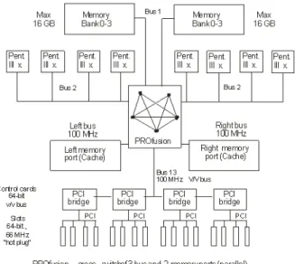
Typical actual example of SMP multiprocessor systems (Intel Xeon) illustrates Fig. 1.

Figure 1. Architecture of SMP parallel computer (8-Intel processor).

From illustrated Fig. 1 we can see that parallel using of computing nodes (processors) requires at least one communication network (at Fig. 1 PROfusion) to realize computing nodes cooperation solving any complex problem in a parallel way. Concretely it means two basic types of communications and that

inter process communications (IPC) of processors via shared memory

access of computing nodes to shared input/output (I/O) devices (I/O communications).

To this time various realized communication network

(switches) mainly in classic parallel computers with shared memory have used topologies or communication networks as follows [2, 25, 32]

deterministic bus (multibus) multistage array crossbar annulus (ring)

mesh, annuloid (torus)

boolean n-dimension cubes (hypercube) butterfly

omega

shuffle (perfect, logarithmic, with exchange, k-routes)

De Bruin network Banyan network Batcher network Benes network

ATM (asynchronous transfer mode) FDDI (Fiber Distributed Data Interface) trees (X-tree, H-tree, fat tree, hyper tree) stochastic

hash networks.

2.1.2. Communication Networks for Parallel Computers with Distributed Memory

For parallel computers with distributed memory (computer networks, cluster, NOW, Grid) the typical used topologies or communication networks are as follows [27, 33]

bus, multibus star

tree ring

Ethernet (Fast, Giga, 10 Giga) high speed communication networks

Myrinet Infiniband Quadrics.

2.2. Communications in Parallel Algorithms

In principal we can divide communication in parallel algorithms (PA) to the following groups

inter process communications in parallel algorithm using shared memory (PAsm). Shared memory (at least a part) allow to use it for communications via I/O instructions of given computing node (processor) or supported parallel developing standards

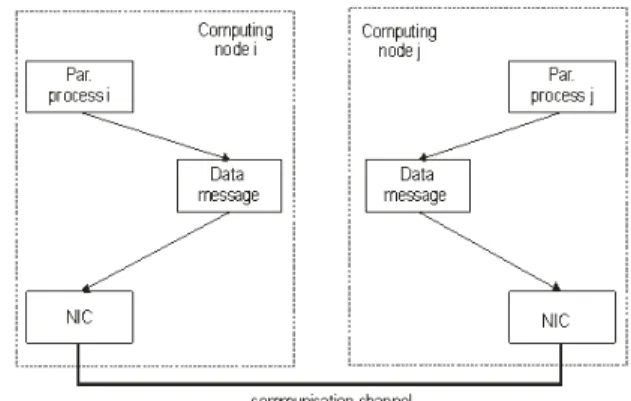
inter process communications in parallel algorithm using distributed memory (PAdm). All needed cooperation of parallel processes have to use only asynchronous data message communication via parallel supported developing standards

The main difference between PAsm and PAdm is in form of inter process communication (IPC) among created parallel processes [5, 17]. Generally we can say that IPC communication in parallel system with shared memory can use more existed communication possibilities (I/O instructions, communication services in shared memory) than in distributed systems (only network communication).

2.2.1. Inter Process Communication

In general we can say that dominated elements of parallel algorithms are their sequential parts (Parallel processes) and inter process communication (IPC) among performed parallel processes.

2.2.1.1. Inter Process Communication in Shared Memory

Inter process communication (IPC) for parallel algorithm with shared memory (PAsm) is defined within supporting developing standards as following

• OpenMP

• OpenMP threads

Pthreads Java threads other.

The concrete communication mechanisms use existence of shared memory which allows every parallel process to story communicating data at some addressed memory place and then another parallel process to read stored data.

2.2.2.2. Inter Process Communication in Distributed Memory

Inter process communication (IPC) for parallel algorithm with distributed memory (PAdm) is defined within supporting developing standards as following

MPI (Message passing interface)

• point to point (PTP) communication commands send commands

receive commands

• collective communication commands

data distribution commands data gathering commands PVM (Parallel virtual machine)

Java (Network communication services) other.

Typical MPI network communication is at Fig. 2. Based on existed communication links MPI contains mentioned collective communication commands.

2.3. Influence of Communications to Performance Tuning

Performance tuning means performance modeling and optimization of PA (effective PA). This step contents modeling and analysis in such a way to minimize the whole execution time of parallel computing. To achieve effective PA depends mainly from following factors

optimal selection of communication networks in parallel computers

minimization of needed inter process

communication and other accompanying overheads

(parallelization, control of PA, waiting times) [16]. In actually dominated asynchronous parallel computers (NOW, Grid) there are necessary to reduce (optimize) mainly number of inter process communications IPC (Communication complexity) for example through possible using of alternative decomposition model.

Figure 2. Typical MPI network communication.

3. Parallel Computing Models

Parallel computational model is an abstract model of parallel computing, which should include overhead and accompanying delays. Model is characterized by the possibility of parallel computers, which are for parallel computing deterministic. Abstraction degree should

characterize also communication structure and

contemporary permit at least approximation of its basic parameters (complexity, performance etc.) [14, 29]. On the other hand approximation accuracy is limited by requirement that abstract communication models have to represent similar parallel computer architectures and parallel algorithms [18]. It is clear that for every specific parallel computer and parallel algorithm too we are able to

create their own communication model, which

characterizes in detail their specific characteristics. Parallel communication models can be classified according various criterions. One of most used criteria is presentation way of model parameters. Typical used communication parameters can be divided into two groups as follows

semantic

communications network architecture

(architecture, channels, control)

communication methods (communication

protocols)

communication delay (latency)

performance (complexity, efficiency). Typical parameters are

working load s for given PA

size of the parallel system p (number of processors)

parallel speed up S(s, p) efficiency E(s, p) isoefficiency w(s)

average time of computation unit tc (instruction, defined computing step etc.)

communication technical parameters

average time to initialize communication (startup time) – ts

average time to transmit data unit (data word) - tw.

3.1. Communication Model with Shared Memory 3.1.1. PRAM Model

Model of parallel computer with shared memory PRAM (Parallel Random Access Machine) was previously used for its high degree of universality and abstractness. PRAM model still represents an idealized model, because it is not considering any delay. Although this approach has an important role in the theoretical design and development of parallel computers and parallel algorithms but for real modeling it is necessary to complete it by modeling at least of communication delays. Typical PRAM model illustrates Fig. 3.

Figure 3. PRAM model.

In PRAM model computing nodes communicate via shared memory whereby every addressed place according PRAM model is available at the same time. Computing nodes are at their activities synchronized and communicate via shared memory. For practical design of a parallel algorithm programmer specifies sequences of parallel operations using shared memory. In performing parallel processes may come to long waiting delays which are increased proportionally to number of used parallel processes [4]. These time delays is necessary to model, analyze their behavior and make their real evaluation (removing of idealized PRAM model assumption).

3.1.1.1. Fixed Communication Model

Fixed communication model GRAM (Graph Random Access Machine) was one of the ways how to solve problem of waiting delays in PRAM model using distributed memory with precisely defined structure of its communication network in which symbol G determines topology graph of used communication network [25]. As

examples we can name two dimensional communication networks and hypercube topology.

3.2. SPMD Model

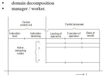
Parallel computing model SPMD (Single Process Multiple Data) corresponded to classical parallel computers with shared memory (supercomputers, massive SMP) which were primary focused on massive data parallelism. Illustration of this model is shown at Fig.4. Such an

orientation program assumes mostly following

decomposition models [1, 17] domain decomposition manager / worker.

Figure 4. SPMD model.

3.3. Flexible Models

Previous models were not sufficiently precise, because increasing robustness of parallel computers cause also rises of communication overheads in parallel algorithms. The precise developed parallel computer represented robustness by number of computing nodes with parameter p, whereby every computing node was ready to work with n / p parallel processes. Parallel algorithm then consisted of sequence of defined parallel steps named as super steps, in which were done needed local calculations followed by communication exchange of data messages. It is obvious that such implemented parallel algorithm, in which number of super steps was small and independent of input load n, will be effective in any parallel computer providing efficient implementation just of communications procedures.

3.3.1. Flexible GRAM Model

Basic difference between fixed and flexible GRAM model is in number of computing nodes (Processors), which was considered with defined parameter p. At every stage of communication phase computing node could send data messages with their variable length to its neighbor computing nodes. Communication prize could be also subject of modeling and included following parts

communication section to initialize communication (Startup time)

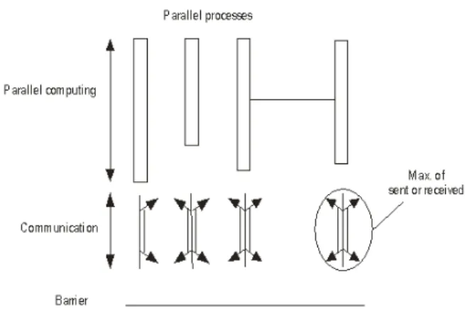
3.3.2. BSP Model

Communication model BSP (Bulk Synchronous Parallel) is a realistic alternative of PRAM model (Fig. 5.). Number of parallel super steps (input load n) was divided to p computing processors. Updates of this communication model have used instead of synchronization after every performed instruction only synchronization at the end of performed partial computation referred as super step. Super step consisted from defined number of instructions (bulk). Each super step consisted of three following phases

own partial computation

global communications of processors barrier synchronization.

At super step used processors are performing their instructions asynchronously, whereby all read operations of collective memory of every processor were performed before performing the first write operation to shared memory. Existing delays of parallel algorithm were defined as follows

parallel computation time were given by the maximum number of computation cycles w

synchronization delay has its lower bound as the

waiting time for transmission of minimal

communication data messages through

communications network

• communication delay was given as the product g.h cycles, where parameter g characterizes throughput of communication network. Parameter h specified number of cycles for communication of maximal data message at super step. To avoid conflicts due to asynchronous communication network activities, send data message in stage by some processor is not dependent on received messages in the same phase of communication execution time for one super step is then given as the sum of the partly considered sub delays and that w + g.h + l.

BSP model does not exclude overlapping of individual super step activities. In the case of overlapping of defined actions execution time of super step were given as max (w, g.h, l).

Figure 5. BSP model.

3.3.2.1. Adjusted BSP Model

Further innovation of BSP model includes adjustments PRAM and BSP models in such a way that modified model could be precisely characterize behavior of real parallel computers. These innovations were based on following

parallel algorithm is performed in sequence of phases. There were following three types of phases and that namely

parallelization overheads T(s, p)overh own parallel computing T(s, p)comp

interaction of computing nodes T(s, p)interact (communication, synchronization).

for given computation phase were determinate input load with parameters that indicate average value of performed operations tc(p)

different interaction imposes different execution times. Execution time could be computed according following relation

( )

_{( ) ( )}

( )

.

) , (

int t p mt p

p r

m p t p m

T _eract = _s + = _s + _c

∞

In this relationship m indicates data message length in bytes, ts(p) is communication start up time and r ∞ (p) is bandwidth limit of used communication channels.

3.3.2.2. CGM (Coarse Grained Multicomputer) Model

This model is based on BSP model and is represented by p processors whereby each of them with O(n / p) local memories for which every super step has h = O(n / p) communication cycles. The aim is to concentrate on a proposal with fewer super steps in order to achieve higher effectiveness of developed parallel algorithms. The ideal situation means to perform constant number of super steps as it was done in developed parallel algorithms as sorting, image processing, optimization problems etc.

3.3.2.3. Log P Model

Log P model is based on BSP model and focuses on a

looser bound parallel computer architectures

(Asynchronous parallel computers).The emphasis is on a parallel computer with distributed memory with parameters according Fig. 6 where

L: time for communication initialization (Startup time)

o: overflow due to communication activities. It is defined as the time interval during which computing node performs only control of performed communication

Figure 6. Log P model.

In this model they are considered the resources with their limited capacity. Consequently then only L / g data messages can be at a given time in communication network. Price for basic communication data block between two computing nodes is L + 2 o. If we require acknowledgement (ACK) then price is given as 2 L 2 + o.

3.4. Communication Models with Distributed Memory 3.4.1. Model MPMD

Computational model MPMD (Multiple Process

Multiple Data) is associated with computer networks mainly in asynchronous parallel computers. As network topologies in computer networks (LAN, WAN) there is typically used following topological structure [6]

bus star tree ring.

Suitable decomposition models are those which tend to functional parallelism, that mean to create of parallel processes, which can then perform allocated part of parallel algorithms on corresponding data. Typical decomposition models are as following [8]

functional decomposition

manager / server (Server / client, master / worker) object oriented programming OOP.

4. Complexity in Communication

Networks

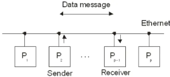
Typical communication network using single shared communication channel is illustrated at Fig. 7. The main disadvantage of such communication network is a serial communication among connected computer nodes. To analyze communication complexity we can apply analytical method of complexity theory. Then upper limit of communication complexity at Ethernet is given as O (p) for

supposed network connection according Fig. 7.

Communication network with this communication

complexity limits development of effective parallel algorithms using serial communications as in case of

Ethernet network.

Figure 7. Communication in Ethernet network.

Typical communication network in NOW is based on Ethernet network. The communication principles in this network are illustrated at Fig. 7 where P1, P2, ... Pp-1, Pp could by common powerful single workstations or SMP parallel computers. Generally implementing computational model MPMD brings different overhead delays as follows

parallelization of complex problem

synchronization of decomposed parallel processes inter process communication (IPC) delay.

All these delays in parallel computers with distributed memory are reflected to communication complexity of used communication network.

Figure 8. Real communication models.

Real application models should take into account potential lack of limited communication channels at implementation of parallel algorithms (technical communication limits) respectively other limited required technical resources [19]. Illustration of resource technical limits illustrates Fig. 8.

4.1. Modeling of Communication Complexity

To model communication complexity in actual parallel computing is of high importance from these causes [20]

it plays important role in achieving high performance of all actual parallel computers (SMP, Now, Grid)

to develop effective PA there is necessary to model and optimize inter process communications mainly for parallel algorithms with distributed memory [10].

parallel algorithms with intensive IPC communications.

Figure 9. Relations among parts of parallel execution time.

We can easily show that limit of processing time T(s, p)comp with increasing number of computing nodes p goes to null using theory of complexity. Processing time complexity T(s, p)comp is given through quotient of running time of the greatest parallel process PP (product of its complexity Zpp and a constant tc as an average value of performed computation operations) through number of used computation nodes of the given parallel computer. Based on them we are able to derive for parallel computation time T(s, p)comp following relation

p t Z s

T comp pp c

. )

p ,

( =

Supposing ideally parallelized problem (for example matrix PA) and theoretical unlimited number of computation nodes p mathematical limit of T(s, p)comp is given as

0 . lim )

p ,

( = _→∞ =

p t Z s

T comp p pp c

For effective parallel algorithms we are seeking for the bottom part of whole execution time according Fig. 9.

4.2. Communication Latencies

Inter process communication of parallel processes (IPC) T(s, p)comm (communication latency) influences in a decisive degree used decomposition model of PA. Obviously it is higher in parallel algorithms with distributed memory PAdm than in other ones. To model communication latency we have applied theory of complexity to inter process communication T(s, p)comm of parallel processes in a similar way as in modeling computation latency T(s, p)comp focusing to a number of

performed communication steps (communication

complexity). Then communication complexity Z(s, p)comm is given through number of performed communication

steps (communication complexity) for used

decomposition model of given PA. Every communication step within parallel computer based on NOW module we

can characterized through two basic communication parameters as follows

communication parameter ts defined as parameter for initialization of communication step (startup time)

communication parameter tw as parameter for transmission latency of considered data unit (typically word).

Illustration of defined communication parameters is at Fig. 10. These communication parameters ts, tw are constants for defined parallel computer [11]. Then the communication latency T(s, p)comm using communication complexity Z(s, p)comm and the defined communication parameters is given as follows

)

(

)

,

(

)

,

(

s

p

_comm

Z

s

p

_comm

t

_s

t

_w

T

=

+

The whole communication latency is given through two basic following functions

function f1(ts) which represents the whole number of communication initializations for given parallel process

function f2(tw) which correspondents to whole performed data unit transmission (usually time of word transmission for given parallel computer) in given parallel process.

Figure 10. Illustration of communication parameters.

These two defined functions limit performance of used parallel computer on defined NOW module of parallel computer. Then using a superposition we can write for communication latency in NOW module T(s, p)comm. as follows

) ( ) ( )

,

(s pcommNOW f1 ts f2 tw

T = +

various communication networks is defined as number of hops [21, 24].

To model communication latency we need to extend the considered two communication functions f1(ts), f2(tw) in NOW module by third function component f3(th), which will determine potential multiple crossing used NOW modules of integrated parallel computer. This third function is characterized through multiplying hops parameter lh among NOW modules (generally u NOW networks) and average communication latency time of jumped NOW modules with the same communication speed or a sum of individual communication latencies for jumped NOW modules with their different communication speed. Then in general to the whole communication latency in Grid is valid

∑

=

+ +

= u

i

h w s w

s

commGRID f t f t f t t l

p s T

1 3 2

1( ) ( ) ( , , )

) , (

In general communication latency time f3(ts, tw, lh) is time to send data message with m words in one communication step among integrated NOW modules with lh hops. The communication time for one communication step is then given as ts+ m tw lh th, where the new parameters are

lh is the number of network hops

m is the number of transmitted data units (usually words)

th is average communication time for one hop. The new communication parameters th, lh depend from a concrete architecture of Grid communication network and used routing algorithm. In [9] we have developed unified models which could help to establish these parameters for dominant parallel computers. For the complex analytical modeling there is necessary to derive for given parallel algorithm or a group of similar algorithms (matrix parallel algorithms) needed communication functions and that always individually for any decomposition strategy) for

known technical parameters (computational,

communication) of used parallel computer (classic, NOW, Grid).

5. Communication Latencies of PA

To this time known results in complexity modeling on the in the world have used mainly classical parallel computers with shared memory (supercomputers) or massive multiprocessors with distributed memory which in most cases did not consider the influences of overheads in parallel computing (communication, synchronization, parallelization, waiting etc.) supposing that they would be lower in comparison to the latency of performed massive parallel computations [22].

In this sense analysis and modeling of complexity in parallel algorithms (PA) are to be reduced to only complexity analysis of own computations T(s, p)comp, that mean that the function of all existed control and

communication overhead latencies h(s, p) were not a part of derived relations for whole parallel execution time T(s, p). In this sense the dominated function in the relation for used isoefficiency function w(s) of the parallel algorithms is complexity of performed massive computations T(s, p)comp. Such assumption has proved to be really true in using classical parallel computers (supercomputers, massive SMP, SIMD architectures etc.). Putting put on this assumption to the relation for asymptotic isoefficiency w(s) we get w(s) as follows

[

T

s

p

comp

h

s

p

]

T

s

p

comp

s

w

(

)

=

max

(

,

)

,

(

,

)

<

(

,

)

In opposite at parallel algorithms for actually dominant parallel computers based on NOW and Grid there is for complex modeling necessary to analyze at least to evaluate most important overheads from all existed overheads which are [8, 10]

architecture of parallel computer T(s, p)arch own computations T(s, p)comp

communication latency T(s, p)comm start - up time (ts)

data unit transmission (tw) routing

parallelization latency T(s, p)par synchronization latency T(s, p)syn

waiting caused by limiting shared technical

resources T(s, p)wait (memory modules,

communication channels etc.).

All these named overhead latencies build in defined is efficiency function the whole overhead function h(s, p). In general the influence of h(s, p) is necessary to take into account in complex performance modeling of parallel algorithms or at least to evaluate their important individual components. The defined overhead function h(s, p) is as follows

(

)

∑

= T s parch T s ppar T s pcommT s psyn p

s

h( , ) ( , ) , ( , ) , ( , ) ( , )

Overhead function T(s, p)arch is projected into used technical parameters tc, ts, tw, which are constants for given parallel computer.

The second overhead function T(s, p)par depend from chosen decomposition strategy and their consequences are projected so to computation part T(s, p)comp as to communication part T(s, p)comm.

The third overhead function T(s, p)syn we can eliminate through optimization of load balancing among individual computing nodes of used parallel computer. For this purpose we would measure performance of individual used computing nodes for given developed parallel algorithm and then based on done measured results we are able to redistribute better given input load. These activities we can repeat until we have optimal redistributed input load (Load balancing).

performance modeling of parallel algorithms. Then for asymptotic isoefficiency analysis of complex performance analysis we should consider w(s) as follows

[

(, ) , ( , )

]

max )

(s T sp h sp

w = _comp

, where the most important parts for dominant parallel computers (NOW, Grid) in overhead function h(s, p) are in relation to done analysis of individual overhead latencies the influence of communication latency of T(s, p)comm.

Then the kernel of asymptotic analyze of h(s, p) is analysis of communication latency T(s, p)comm including projected consequences of used decomposition methods. In general derived isoefficiency function w(s) could have nonlinear character at gradually increasing number of computing nodes p. Analytical deriving of isoefficiency function w(s) including communication latency T(s, p)comm allow us to predict PA performance of given parallel algorithm so for real as for hypothetical parallel computers.

6. Applied Modeling of Communication

Latency

We will illustrate modeling process of communication latency on approximation solution of steady state solution Ф (x, y) for points in the interior by the function u (x, y) according Fig. 11. Given a two dimensional region and values for points of the region boundaries, We can do this by covering the region with a grid of points and to obtain the values of u (xi, yj) = ui,j of the area. Each inner point is initialized to some initial value. Other stationary values of inner points will by computed applying iterative methods. In each iteration step, the new point value (next) will be defined as average of previous (old) or a combination of previous and new set of values of neighboring points. Iterative computation ends either after performed fixed number of iterations or after reaching defined precision acceptable difference E > 0 (epsilon value) for each new value. Epsilon accuracy is determined as desired difference between the previous and the new point value.

Figure 11. Grid approximation of two dimensional region.

These limits of points that indicate the boundary conditions as follows

according to Dirichlet [10] giving the values of given function analyzed function at both ends of the field (at U = 0 for x = 0, 0 ≤ Y ≤ 1, U = 1 for X = 1,

0 ≤ Y ≤ 1)

according to the Neumann [10] giving the values with solution derivations (for example uy= 0 for Y = 0, 0 ≤ X ≤ 1, uy = 0 for Y = 1 0 ≤ X ≤ 1).

To model communication complexity we will represent two dimensional grid of points with matrix in abstract form that means for empty matrix. Then we are considering the typical following n x m matrix

A =

a , a , … , a a , a , … , a . . . . . . . . . a , a , … , a

To reduce number of variables in deriving modeling process we will consider matrix with m = n (square matrix). For this purpose there are also following causes

• we can transform any matrix n x m to n x n matrix through expanding rows (if m < n) or columns (if m > n)

• derivation process will be the same only when considering the workload instead of n2 (square matrix) we should consider n x m (oblong matrix).

Communication model structure is involved in the communication complexity of the parallel algorithm. We would analyze the basic communication requirements potential using of iterative method. Analysis via iterative methods is based on iterative computation of the new iterative value of given internal point from fixed number of neighboring points according concrete iterative relationship. To compute each new value of one point of approximated network points they are setting to used iteration relation set of specified number of neighboring point values (iteration step). In our case it could be derived to compute the new value X I, j on a two dimensional network of points iterative relation where each new point value is computed as the arithmetic average of the four neighboring points as follows

Xi, j(t +1) = (Xi-1, j(t) + Xi +1, j(t) + Xi, j-1(t) + Xi, j +1(t)) / 4

Iterative calculation according to the following iterative relationship and are repeated sequentially in each iteration step, the new gain values Xi, j(1), Xi, j(2)...etc., while the name Xi, j(t) determines the value at a given point Xi, j t - step. Suppose applying decomposition models create parallel processes for each point, respectively group of points as the two-dimensional network points.

Figure 12. Communication for 4 - point approximation.

The needed communication process is as follows for t = 0 to t–1 do

begin

send Xi,j(t) to each neighbor;

receive Xi-1,j(t),Xi+1,j(t),Xi,j-1(t),Xi,j+1(t) from the neighbors; compute Xi,j(t+1) using the specified iteration relation for Xi; end;

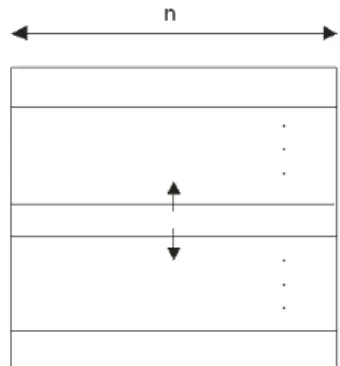
6.1. Matrix Decomposition to Strips

Decomposition method to rows or columns (Strips) are algorithmic the same and for their practical using is critical the way how are the matrix elements putting down to matrix.

Figure 13. Communication consequences for decomposition to strips

(rows).

In this way it is possible send very simple through specification of the beginning address for a given row and through a number of elements in row. Let for every parallel process (strips) two messages are send to neighboring processors and in the same way two messages are received from neighboring processors (Fig. 13) supposing that it is possible to transmit for example one row to one message. Communication time for a calculation step T(s, p)coms is then given as

(

)

4

)

,

(

s

p

comms

t

s

n

t

w

T

=

+

Using these variables for the communication overheads in decomposition method to strips is correct

)

t

(t

4

)

,

(

)

,

(

)

p

,

(

s

T

s

p

h

s

p

s

n

w

T

comm

=

comms

=

=

+

In this case a communication time for one calculation step does not depend on the number of used calculation processors.

6.1.1. Matrix Decomposition to Blocks

For mapping matrix elements in blocks a inter process communication is performed on the four neighboring edges of blocks, which it is necessary in computation flow to exchange. Every parallel process therefore sends four messages and in the same way they receive four messages at the end of every calculation step (Fig. 14.) supposing that all needed data at every edge are sent as a part of any message).

Figure 14. Communication model for decomposition to blocks.

Then the requested communication time for this decomposition method is given as

) (

8 )

,

( _{commb s} t_w p n t p

s

T = +

This equation is correct for p ≥ 9, because only under this assumption it is possible to build at least one square because only then is possible to build one square block with for communication edges. Using these variables for the communication overheads in decomposition method to blocks is correct

) (

8 ) , ( )

, ( ) p ,

( comm commb s tw

p n t p s h p

s T s

T = = = +

Then the requested communication time for this decomposition method is given as

) (

8 s w

comb t

p n t

T = +

Data exchange at all shared edges points for both decomposition strategies (blocks, strips) illustrates Fig. 15.

6.1.2. Optimization of Decomposition Model Selection

For comparison based on derived relations for communication complexity decomposition method to

blocks demands higher communication time as

decomposition to strips (more effective decomposition to strips) if

) ( 4 ) (

8 _s t_w t_s nt_w p

n

t + > +

or after adjusting for technical parameter ts.

. ) 2 1

( _w

s t

p n

t > −

or for second technical parameter tw as follows

. ) 2 1

( s

w t

p n

t > −

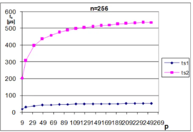
This relation is valid under assumption that p ≥ 9, which is real condition in developed iterative parallel algorithms to build real square block. Fig. 16 illustrates choice optimization of suitable decomposition method based on derived dependences to establishing ts for n = 256 and following values of tw

• tw = 230 ns = 0,23 µs (NOW IBM SP-2) • tw = 2,4 µs (NCUBE 2).

For higher values ts as at given tsi (ts1for tw = 0, 23 µs and ts2 for tw = 2, 4 µs) from the appropriate curve line for n = 256 is more effective decomposition method to strips. Limited values in choice optimal decomposition strategy are at given n for higher values tw. Therefore in general decomposition to strips is more effective for higher values of ts.

Figure 16. Optimization of decomposition method.

Threshold values ts to select the optimal model of matrix decomposition strategy are for given n for larger values of tw greater. Then in generally decomposed into strips (rows, columns) is more effective for higher values of ts (NOW, Grid) and decomposition into blocks again for smaller values of ts (classic massive SMP, supercomputers etc.). Generally the times of ts are significant higher for parallel computers as NOW and Grid. For example NOW for FDDI

based optical cables with ts = 1100 µs, tw = 1.1 µs and for architecture with Ethernet ts= 1500 µs, tw= 5 µs) [8]. In such systems, the use of matrix decomposition method to strips then more effectively.

7. Measurement of Communication

Latency

For experimental measurements of PA delays we can use available services of used parallel development environment (MPI services, Win API 32, Win API 64, etc.). For example to measurement of execution time of parallel processes we have been used following functions Win 32 API and Win API 64

• Query Performance Counter which returns actual value of counter

• Query Performance Frequency which defines counting frequency per second.

Values of both functions depend on used computer nodes. Using of above measuring time functions we can obtain execution times with high accuracy. For example for common Intel Pentium processors or higher it is 0.0008 ms which is sufficient for the time analysis of PA.

To measure communication latencies we can define function to measure time between two points of performed parallel algorithm respectively parallel process. An example of following pseudo code to measure time between two points T1 and T2 is as follows

T1: time (&t1); /*start of time*/ T2: time (&t2); /*stop time*/

measured_ time = difftime (t2,t1); /*measured time = t2-t1*/

printf (“Measured time = % 5.2 f ms“, measured_time); Illustrated approach is for measurement of monitoring times universal that is we can use it so for measurements of parallel algorithms as for measuring monitoring overheads of parallel processes, or measuring delays which are typical to establish technical parameters of parallel computers.

7.1. Communication Technical Parameters 7.1.1. Classic Parallel Computers

We have been derived relations to communication comparisons of possible matrix decomposition models. We have been derived that decomposition model to strips (rows, columns) demands lower inter process communication delays than decomposition model to blocks with respecting derived condition that for blocks p ≥ 9, for communication parameter ts according following inequality

) 2 1 (

p t

n t_s > _w −

parallel algorithms MPA from this is resulting allocation of n = p. In case of massive equations in which n > p computing nodes will be repeatedly perform needed algorithm activities for remaining n > p strips (rows, columns). For example if we supposed for simplicity that the value of parameter n is divisible through parameter p without rest, used computing nodes of parallel computers will be repeatedly perform k times needed algorithm activities till exhausting quotient value of k = n/p. For both complexities (computation, communication) it mean k – multiplying factor of both mentioned complexities as derived complexities for pre n = p. From this fact it is clear that the base outgoing problem is to derive so computational as communication complexity for given n = p. Setting previous equality to the relation for technical parameter ts after needed performed adjustments we get finally following relation

) 2

(n n

t t_s > _w −

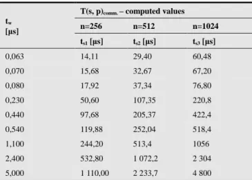
In Tab. 1 we have computed the values ts for known values of communication parameter tw [7, 15].

Table 1. Optimization of decomposition method for ts.

tw

[µs]

T(s, p)comm. – computed values

n=256 n=512 n=1024

ts1 [µs] ts2 [µs] ts3 [µs]

0,063 14,11 29,40 60,48

0,070 15,68 32,67 67,20

0,080 17,92 37,34 76,80

0,230 50,60 107,35 220,8

0,440 97,68 205,37 422,4

0,540 119,88 252,04 518,4

1,100 244,20 513,4 1056

2,400 532,80 1 072,2 2 304

5,000 1 110,00 2 233,7 4 800

Graphical illustrations of optimal decomposition strategy for computed values in Tab. 1 are illustrated are at Fig. 17 (smaller values of ts) and Fig. 18 (higher values of ts).

Figure 17. Optimization of decomposition methods for smaller values of ts.

Figure 18. Optimization of decomposition methods for higher values ts.

This inequality for ts we are able modified for other input parameter (tw, n) and compute remaining parameter. For example after adjustment for value of parameter tw is valid

n n

t

t s

w

2

− <

At Tab. 2 we have been computed the values tw for known values of communication parameter ts [7, 15].

Table 2. Optimization of decomposition method for tw.

ts

[µs]

T(s, p)comm. – computed values

n=256 (224) n=512 (466,75) n=1024 (960) tw1 [µs] tw2 [µs] tw3 [µs]

3 0,01339 0,0064 0,0031

35 0,01560 0,0750 0,0365

64 0,2857 0,1371 0,0666

77 0,3437 0,1650 0,0802

82 0,3661 0,1757 0,0854

87 0,3884 0,1864 0,0906

154 0,6875 0,3299 0,1604

1 150 5,1339 2,4638 1,1979

1 500 6,6964 3,2137 1,5625

Limiting values for optimal selection of decomposition strategy will be at given n for higher values of tw also higher. Then decomposition model to strips will be more effective for higher values of ts (NOW, Grid) and decomposition models to blocks for lower values of ts.

7.2. NOW Parallel Computer

For analyzed decomposition models we are going to analyze generally their communication complexity.

Communication function T(s, p)comm for given

decomposition strategy is principally defined in NOW with defined two communications parameters and that namely

• communication latency due to parameter ts • communication latency due to parameter tw.

an analytical way relations of all MPI collective communication commands in Ethernet. There is possible to evaluate it also for other concrete communication network architectures.

7.2.1. Evaluation of Collective Communication Mechanisms

For the following typical MPI communication

mechanisms on the Ethernet network are valid the following relationships

• MPI command of data dispersion MPI command Broadcast MPI command Scatter • MPI command of data collection

MPI command Gather MPI command All gather MPI command Reduce.

7.2.2. Collective Communication Mechanism Type Broadcast

Collective communication mechanism Broadcast is the only collective communication mechanism that can be effective also in Ethernet communications network. In this case of transmission of one of the same data unit (Byte, word) to all other p computing nodes (Processors) in terms of Ethernet network. Communication complexity T(s, p)comm of this command is O(1) respectively using of established communication parameters ts, tw as

w s

commbr t t

p s

T( , ) = +

To transmit data units various m always only one processor (Point to point) computational complexity is given as O(m), respectively supporting communication parameters established by the following formula

) ( )

,

(s p _commbr m t_s t_w

T = +

For transmission of different data unit’s m-1 remaining processor computational complexity is given by O(p), respectively with the support of established communication parameters as

∑

− =

+ =

1

1

) ( )

, (

p

i

w s

commbr mt t

p s T

The same communication delays are for any other

collective communication mechanisms of Ethernet

communication network. Communication complexity T(s, p)commEth common relationship will be determined as

) ( ) 1 ( ) ( )

, (

1

1

w s p

i

w s

commEth mt t p m t t

p s

T =

∑

+ = − +

−

=

In general the value of the parameter ts is highly significant for asynchronous parallel computers NOW and Grid. For example for parallel computer NOW based on fiber optic cable these communication parameters have

concrete values and that ts = 1100 µs and tw = 1,1 µs and for Ethernet communication network are these parameters even higher and that ts = 1500 µs a tw = 5 µ s. The realized measurements in our home conditions (DTI Dubnica and University of Zilina, Slovakia) of these communication parameters on an unloaded Ethernet network were higher than previous specified values. Causes for the substantial differences are mainly the following

• built sophisticated technical support to data block transmission based on direct memory access (DMA) for collective communication mechanisms

• multiple transmission channels based on multistage structure of communication network

• high speed communication network switches named as HPS (High Performance Switch)

• used high speed communications network as Infiniband, Quadrics and Myrinet [34].

8. Conclusions

Modeling of communication latency as a discipline has repeatedly proved to be critical for design and successful use of parallel computers and parallel algorithms too. At the early stage of design, communication models can be used to project the system performance, scalability and evaluate design alternatives [26, 30]. At the production stage, communication evaluation methodologies can be used to detect bottlenecks and subsequently suggests ways to alleviate them. Analytical methods (order analysis, queuing theory systems), simulation, experimental measurements, and hybrid modeling methods could be successfully used for the evaluation of system and its components too [14, 23]. Via the extended form of theory of complexity to modeling of communication latency we are able to predicate communication latency behavior also in other applied parallel algorithms than analyzed matrix decomposition models.

Acknowledgements

This work was done within the project “Complex modeling, optimization and prediction of parallel computers and algorithms” at University of Zilina, Slovakia. The author gratefully acknowledges help of project supervisor Prof. Ing. Ivan Hanuliak, PhD.

References

[1] Abderazek A. B., Multicore systems on chip - Practical Software/Hardware design, Imperial college press, UK, pp. 200, 2010

[2] Arie M.C.A. Koster Arie M.C.A., Munoz Xavier, Graphs and Algorithms in Communication Networks, Springer Verlag, Germany, pp. 426, 2010

[3] Arora S., Barak B., Computational complexity - A modern Approach, Cambridge University Press, UK, pp. 573, 2009 [4] Barria A. J., Communication network and computer systems,

Imperial College Press, UK, pp. 276, 2006

[5] Casanova H., Legrand A., Robert Y., Parallel algorithms, CRC Press, USA, 2008

[6] Dubois M., Annavaram M., Stenstrom P., Parallel computer organization and design, UK, pp. 560, 2012

[7] Hager G., Wellein G., Introduction to High Performance Computing for Scientists and Engineers, CRC Press, USA, pp. 356, 2010

[8] Hanuliak P., Analytical method of performance prediction in parallel algorithms, The Open Cybernetics and Systemics Journal, Vol. 6, Bentham, UK, pp. 38-47, 2012

[9] Hanuliak M., Unified analytical models of parallel and distributed computing, American J. of Networks and Communication, Science PG, Vol. 3, No. 1, USA, pp. 1-12, 2014

[10] Hanuliak P., Hanuliak I., Performance evaluation of iterative parallel algorithms, Kybernetes, Vol. 39, No.1/ 2010, UK, pp. 107- 126

[11] Hanuliak M., Modeling of parallel computers based on network of computing nodes, American J. of Networks and Communication, Science PG, Vol. 3, USA, 2014

[12] Hanuliak P., Complex modeling of matrix parallel algorithms, American J. of Networks and Communication, Science PG, Vol. 3, USA, 2014

[13] Hanuliak M., Hanuliak I., To the correction of analytical models for computer based communication systems, Kybernetes, Vol. 35, No. 9, UK, pp. 1492-1504, 2006 [14] Harchol-Balter Mor, Performance modeling and design of

computer systems, Cambridge University Press, UK, pp. 576, 2013

[15] Hwang K. and coll., Distributed and Parallel Computing, Morgan Kaufmann, USA, pp. 472, 2011

[16] Kshemkalyani A. D., Singhal M., Distributed Computing, University of Illinois, Cambridge University Press, UK, pp. 756, 2011

[17] Kirk D. B., Hwu W. W., Programming massively parallel processors, Morgan Kaufmann, USA, pp. 280, 2010 [18] Kostin A., Ilushechkina L., Modeling and simulation of

distributed systems, Imperial College Press, USA, pp. 440, 2010

[19] Kumar A., Manjunath D., Kuri J., Communication Networking , Morgan Kaufmann, USA, pp. 750, 2004 [20] Kushilevitz E., Nissan N., Communication Complexity,

Cambridge University Press, UK, pp. 208, 2006,

[21] Le Boudec Jean-Yves, Performance evaluation of computer and communication systems, CRC Press, USA, pp. 300, 2011

[22] McCabe J., D., Network analysis, architecture, and design (3rd edition), Elsevier/ Morgan Kaufmann, USA, pp. 496, 2010

[23] Meerschaert M., Mathematical modeling (4-th edition), Elsevier, pp. 384, 2013

[24] Misra Ch. S., Woungang I., Selected topics in communication network and distributed systems, Imperial college press, UK, pp. 808, 2010

[25] Mieghem P. V., Graph spectra for Complex Networks, Cambridge University Press, UK, pp. 362, 2010

[26] Park K., Willinger W., Self-Similar Network Traffic and Performance Evaluation, John Wiley & Sons, Inc., USA, pp. 558, 2000

[27] Peterson L. L., Davie B. C., Computer networks – a system approach, Morgan Kaufmann, USA, pp. 920, 2011

[28] Resch M. M., Supercomputers in Grids, Int. J. of Grid and HPC, No.1, Germany, pp. 1 - 9, 2009

[29] Riano l., McGinity T.M., Quantifying the role of complexity in a system´s performance, Evolving Systems, Springer Verlag, Germany, pp. 189 – 198, 2011

[30] Ross S. M., Introduction to Probability Models, 10th edition, Academic Press, Elsevier Science, Netherland, pp. 800, 2010

[31] Wang L., Jie Wei., Chen J., Grid Computing: Infrastructure, Service, and Application, CRC Press, USA, 2009

[32] Wolf Marilyn, High-Performance Embedded Computing (Second Edition), Morgan Kaufmann, USA, pp. 600, 2014 [33] Zhuge Hai., The Knowledge Grid, Imperial College Press,

USA , pp. 360, December 2011 www pages