Part III
6
Exploratory and Confi rmatory Factor
Analysis
Rex Kline
6.1 Introduction to Exploratory and Confi rmatory Factor Analysis
Factor analysis is a widely used set of techniques in the behavioral sciences. It is also a primary technique for many researchers, especially those who conduct assessment-related studies. The basic logic and mathematics of factor analysis were fi rst described by Charles Spearman (1904b), and many variations of factor analysis were developed over the fol-lowing century. Factor analysis is unique among multivariate statistical procedures in that it was developed mainly by psychologists in order to test hypotheses about the correspon-dence between scores on observed (manifest) variables, or indicators, and hypothetical constructs (latent variables), or factors, presumed to affect those scores. Spearman and his contemporaries (e.g., Thomson, 1920) used factor analysis to evaluate models about the nature and organization of intelligence. Factor analysis is still widely used today in mental test studies as it is in many other research areas as a means to discover and identify latent variables, given initially only sample covariances among a set of indicators (Mulaik, 1987).
Over the years there have been thousands of published factor analytic studies (e.g., Costello & Osborne, 2005), so the impact of factor analysis in terms of sheer volume of the research literature is undeniable. Whether the typical factor analytic study also makes a substantive contribution, however, has been a matter of longstanding debate (e.g., Furfey & Daly, 1937). One challenge is that factor analysis has many decision points. This aspect of the technique is diffi cult for novices, who must navigate the analysis through a myriad of options about variable selection and sampling, the form of the input data, the method of factor extraction, and interpretive strategies, to name a few. A series of bad choices can compromise the results. It is also does not help that default options in some computer procedures for factor analysis are not actually the best choices in many studies. Based on critical reviews of the use of factor analysis in several different research areas (e.g., Fabrigar, Wegener, MacCallum, & Strahan, 1999; Watson & D. Thompson, 2006), it seems that many, if not most, factor analytic studies have at least one serious fl aw. Common problems include sample sizes that are too small and failure to report suffi cient numerical results so that the work can be critically evaluated.
6.2 Theoretical Foundations of Factor Analysis
Spearman (1904a) is also credited with articulating basic principles of classical measure-ment theory and, not surprisingly, there is close connection between factor analysis and psychometrics. In the latter, an observed score Xij for person i measured at time j is
under-stood as made up of a true component Ti and an error component Eij, or
ij i ij
Because measurement error is random and thus unrelated to true scores, variance in ob-served scores can be broken down into two nonoverlapping parts, or
2 2 2
X T E
(6.2)
Score reliability coeffi cients calculated in samples estimate the ratio of true score variance over total observed variance, or
2 2 ˆ / ˆ
XX T X
r (6.3)
and the quantity 1– rXX estimates the proportion of total variance due to measurement error. For example, if rXX = .80, then 1– .80 = .20, or 20% of the total variance is due to error.
Factor analysis further partitions true variance into common variance and specifi c
vari-ance. Common variance is shared among a set of indicators and is a basis for
intercor-relations among them that depart appreciably from zero. In factor analysis, it is generally assumed that (a) common variance is due to the effects of underlying factors and (b) the number of factors of substantive interest is less than the number of indicators. It is impos-sible to estimate more common factors than indicators, but for parsimony’s sake, there is no point in retaining a model with just as many explanatory entities (factors) as there are entities to be explained (indicators) (Mulaik, 2009). The goal of most factor analyses is thus to identify and interpret a smaller number of factors that explains most of the com-mon variance.
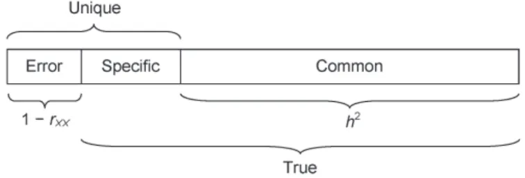
The proportion of total variance that is common is called communality, which is esti-mated by the statistic h2. For example, if h2 = .70, then 70% of total indicator variance
is common and thus potentially explained by underlying factors. The rest, or 30% of the total variance, is unique variance, which is made up of specifi c variance (systematic but unshared) and measurement (random) error. Specifi c variance is not explained by com-mon factors; instead, it may be due to characteristics of individual indicators, such as the particular stimuli that make up a task, that also affect observed scores. The various parti-tions of standardized total indicator variance in factor analysis just described is illustrated in Figure 6.1.
Note in the fi gure that as the proportion of error variance increases, the proportion of systematic (true) variance decreases, which can in turn reduce the overall proportion of common variance. Statistical analysis of unreliable scores usually leads to inaccurate results, and factor analysis is no exception. In general, score reliabilities that exceed .90 are considered excellent, coeffi cients in the range of about .80 are considered good, but coeffi cients appreciably less than .70 are potentially problematic. If rXX < .50, then most
Figure 6.1 Basic partition of standardized indicator variance in factor analysis. h2, proportion of
of total variance is due to measurement error. Indicators with such low score reliabilities should be excluded from the analysis.
6.3 Kinds of Factor Analysis
There are two broad categories of factor analysis, exploratory (EFA) and confi rma-tory (CFA). Differences between these two techniques are listed next and then discussed afterward:
1. Unrestricted measurement models are estimated in EFA, but it is restricted
measure-ment models that are analyzed in CFA. This means that the researcher must explicitly
specify the indicator-factor correspondence in CFA, but there is no option to do so in EFA.
2. Unrestricted measurement models in EFA are not identifi ed, which means there is no unique set of statistical estimates for a particular model. This property concerns the rotation phase, which is part of most applications of EFA. In contrast, CFA models must be identifi ed before they can be analyzed, which means that there is only one exclusive set of estimates. Accordingly, there is no rotation phase in CFA.
3. It is assumed in EFA that the specifi c variance of each indicator is not shared with that of any other indicator. In contrast, CFA permits, depending on the model, estimation of whether specifi c variance is shared between pairs of indicators.
4. Output from CFA computer procedures contains the values of numerous fi t statistics that assess the fi t of the whole model to the data. In contrast, fi t statistics are not gen-erally available in standard methods of EFA (including principle components analysis and principle axis factoring, defi ned later) carried out by computer programs for gen-eral statistical analyses, such as SPSS (IBM, Corp, 2012) and SAS/STAT (SAS Institute, Inc., 2012), but some more specialized computer programs, such as Mplus (Muthén & Muthén, 1998–2012), may print certain types of fi t statistics for particular EFA methods.
5. Procedures for EFA are available in many computer tools for general statistical analy-ses, such as SPSS and SAS/STAT. In contrast, more specialized computer tools for structural equation modeling (SEM) are needed for CFA because the latter is the SEM technique for estimating restricted measurement models. Some widely used SEM com-puter tools include LISREL (Jöreskog & Sörbom, 2012) and Mplus (e.g., Kline, 2010, Chapter 4). The Mplus program has capabilities for both EFA and CFA.
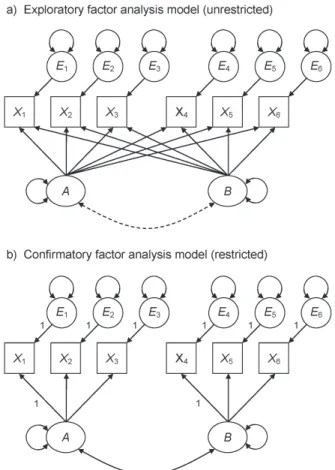
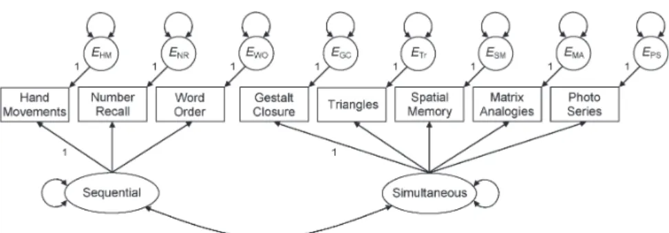
Presented in Figure 6.2 are two hypothetical measurement models for six indicators and two factors represented with symbols from SEM. These include squares or rectangles for observed variables, ellipses or circles for latent variables or error terms, lines with a single arrowhead (→) for presumed direct effects from causal variables to variables affected by them, two-headed curved arrows that exit and re-enter the same variable ( ) for vari-ances of factors or error terms; and curved line with two arrowheads ( ) for covariances (in the unstandardized solution) or correlations (in the standardized one) between either pairs of factors or pairs of error terms (Kline, 2010, chap. 5).
Depicted in Figure 6.2(a) is an unrestricted two-factor model of the kind analyzed in EFA. Without specifi c instruction from the user to do otherwise, an EFA computer proce-dure could theoretically generate all possible unrestricted factor solutions, which equals the number of indicators. The most basic solution is a single-factor model, which refl ects the assumption that all indicators depend on just one common factor. Next is a two-factor model, then a three-factor model, and so on up to the most complex model possible with just as many factors as indicators. In practice, EFA computer procedures rely on default
statistical criteria for determining the number of factors to retain, but these defaults do not always correspond to best practice. These issues are elaborated later in the section about EFA, but the point now is that EFA does not require the researcher to specify the number of factors in advance.
The model in Figure 6.2(a) is unrestricted concerning the correspondence between in-dicators and factors. In EFA, each indicator is regressed on every factor in the model. The statistical estimates for this part of EFA are actually regression coeffi cients that may be in either standardized or unstandardized form, just as in the technique of multiple regres-sion. The difference is that predictors in ordinary regression are observed variables, but the predictors in EFA (and CFA, too) are latent variables. For example, there are two lines with single arrowheads that point to indicator X1 from each of the factors in Figure 6.2(a).
These paths represent the presumed direct effects of both factors on X1, and the proper
name of the statistical estimates of these effects is pattern coeffi cients. Many researchers refer to pattern coeffi cients as “factor loadings” or just “loadings,” but this term is inher-ently ambiguous for reasons explained later and thus is not used here. The larger point is that all possible pattern coeffi cients are calculated for each indicator in EFA.
Pattern coeffi cients in factor analysis are interpreted just as coeffi cients in standard mul-tiple regression.1 Suppose that the unstandardized pattern coeffi cient for the path A → X
1
Figure 6.2 An exploratory factor analysis model and a confi rmatory factor analysis model for
is 5.25 and that the standardized pattern coeffi cient for same path is .60. These results in-dicate that, respectively, (a) a difference of 1point on factor A predicts a difference of 5.25 points in the raw score metric of X1, controlling for the other factors, and (b) a difference
of a full standard deviation on factor A predicts a difference of .60 standard deviations on
X1, again controlling for all other factors. In multiple regression, standardized coeffi cients
are not generally correlation coeffi cients when the predictors covary. It is only in the very special case where all intercorrelations among the predictors are zero that standardized regression coeffi cients are interpreted as correlations. The same distinction holds in factor analysis: When the factors are correlated, the value of an indicator’s standardized pattern coeffi cient will not typically equal that of its structure coeffi cient, which is the estimated correlation between an observed variable and a latent variable. It is only when the fac-tors are independent that standardized pattern coeffi cients will equal the corresponding structure coeffi cient for every indicator. The failure to correctly distinguish standardized pattern coeffi cients from structure correlations when the factors are correlated can lead to misinterpretation of the results (Graham, Guthrie, & Thompson, 2003).
Each indicator in Figure 6.2(a) has an error term, which represents unique variance in factor analysis (see Figure 6.1). The curved line with two arrowheads in the fi gure repre-sents in EFA the possibility to estimate the correlation (or covariance in the unstandard-ized solution) between factors A and B. Because it is not required in EFA to estimate factor correlations, the curve of the symbol in Figure 6.2(a) is presented as dashed instead of solid. When factor correlations are not estimated in EFA, it is assumed that the factors are orthogonal, or all pairwise independent. Most EFA computer procedures by default do not analyze correlated factors. Instead, the user must typically specify a rotation option that permits the factor to covary when the goal is to analyze correlated factors. Whether the computer default to analyze orthogonal factors makes theoretical sense in most ap-plications of EFA is considered later.
Presented in Figure 6.2(b) is a restricted measurement model for two factors and six indi-cators of the kind analyzed in CFA. In the guise of its covariance structure, the model in Figure 6.2(b) represents the hypotheses that indicators X1 – X3 measure factor A,
indica-tors X4 – X6 measure factor B, and the factors covary. This particular model is a standard
CFA model with the characteristics listed next:
1. Each indicator is represented as having two causes—a single factor that the indicator is supposed to measure and all other unique sources of infl uence represented by the error term (e.g., A X1 E1). In CFA models with 2 factors, this property implies
that some pattern coeffi cients are zero. For example, there is no path that connects factor B with indicator X1 in Figure 6.2(b). This specifi cation refl ects the hypothesis
that X1 does not depend on B . It also implies that the pattern coeffi cient for the direct
effect of B on X1 is assumed to equal zero and, consequently, the computer will not
estimate this direct effect. As mentioned, it is the researcher who specifi es the particu-lar pattern coeffi cients to be estimated in CFA, not the computer as in EFA.
2. All possible pairs of factors are assumed to covary in CFA models. This assumption is represented in Figure 6.2(b) by the specifi cation A B, where the curve in the symbol is shown as solid instead of dashed. In models with 3 factors, every pair of factors is connected by the symbol for a covariance. Although it is theoretically possible in CFA to analyze a measurement models where some factors are assumed to be unrelated, such models are not standard models. In fact, some SEM computer tools automatically specify correlations between every pair factors in CFA measurement models.
3. The error terms in the CFA model of Figure 6.2(b) are independent of each other, which refl ects the same assumption as in EFA that indicator specifi c variances do not overlap. However, it may be possible in CFA to estimate error correlations (standard-ized) or error covariances (unstandard(standard-ized) between some pairs of indicators. Suppose that X1 and X7 are the only two indicators in a larger set based on the self-report
method. Because they share a common method, scores on X1 and X7 may covary even
if each indicator depends on a different factor. Specifi c variances of repeated measures variables may also overlap, a pattern called autocorrelation. Correlated errors are represented in CFA model diagrams with the same symbol as for factor correlations, such as E1 E7 for the indicator pair X1 and X7.
Standard CFA models specify unidimensional measurement for all indicators. There are two different ways to specify multidimensional measurement, which also implies a
non-standard CFA model: if any indicator is regressed on 2 or more factors (i.e., there
are 2 pattern coeffi cients for the same indicator) or if correlated errors are specifi ed. For example, adding the direct effect B X1 to the model of Figure 6.2(b) would specify
multidimensional measurement. There is controversy about allowing indicators to depend on more than one factor. On the one hand, some indicators may actually measure more than one domain. An engineering aptitude test with text and diagrams, for instance, may measure both verbal and visual-spatial reasoning. On the other hand, unidimensional models offer more precise tests of convergent validity and discriminant validity. A set of variables presumed to measure the same construct shows convergent validity if their inter-correlations are at least moderate in magnitude. In contrast, a set of variables presumed to measure different constructs shows discriminant validity if their intercorrelations are not too high. If rXY = .90, for instance, then we can hardly say that variables X and Y measure distinct constructs.
The numerals (1) that appear in Figure 6.2(b) next to paths that point to indicators or error terms are scaling constants that represent the assignment of a scale or metric. Because factors and error terms are not directly measured, they require a scale before the computer can generate statistical estimates for them. For example, the specifi cation
1 1 1.0
E X
in Figure 6.2(b) scales the error term so that its variance is related to that of the unex-plained variance in the corresponding indicator. The specifi cations
1 1.0 and 4 1.0
AX BX
in the fi gure scale the factors such that their variances are related to that of the explained (common) variance of the corresponding indicator. Because the scales of X1 and X4 are
“borrowed” in order to scale the factors, each of these indicators is a reference variable. Assuming that indicators of the same factor have equally reliable scores, it is actually arbi-trary which indicator is selected as the reference variable, but both factors and error terms must be assigned scales in CFA (and in SEM, too). Some SEM computer programs, such as LISREL and Mplus, scale factors and error terms automatically, but other programs may require the user to explicitly scale each of these variables. There are actually scaling constants in EFA, but computer procedures for EFA automatically assign these constants as part of the analysis.
Readers should not overinterpret the labels “exploratory” and “confi rmatory.” It is true that EFA does not require a priori hypotheses about factor-indicator correspondence or
even the number of factors. However, there are ways to conduct EFA in a more confi rma-tory mode, such as instructing the computer to extract a certain number of factors based on theory. Also, the technique of CFA is not strictly confi rmatory. Specifi cally, it happens in perhaps most analyses that the initial restricted measurement model does not fi t the data. In this case, the researcher typically modifi es the hypotheses on which the initial model was based and specifi es a revised model. The respecifi ed model is then tested again with the same data. The goal of this process is to “discover” a model with three proper-ties: It makes theoretical sense, it is reasonably parsimonious, and its correspondence to the data is acceptably close.
This is a good point to mention two critical issues in factor analysis. One is the
fac-tor indeterminacy problem, which is that hypothetical constructs can basically never be
uniquely determined by their indicators. This means that although the results of a factor analysis might indicate that a particular measurement model is consistent with observed covariances, there may be nevertheless be other factor structures just as consistent with the same data. A more modern expression of the same idea refers to the problem of equivalent
models, and for measurement models with multiple factors there are actually infi nitely
many equivalent versions. This is not a fatal fl aw of factor analysis but instead a charac-teristic of statistical modeling in general. As noted by Mulaik (1987), such techniques are best seen as hypothesis-generating methods that support inductive reasoning but do not produce defi nitive, incontrovertible results. The second critical issue concerns the naming
fallacy, or the false belief that the name assigned to a factor by a researcher means that the
hypothetical construct is understood or even correctly labeled. Factor names are descrip-tions, not explanadescrip-tions, so we cannot assume that a particular factor label is necessarily the correct one. An example where the same two factors are assigned different labels by different researchers is presented later, but factor labels should be considered as hypoth-eses and not as substitutes for critical thinking.
6.4 Decision Points in Factor Analysis
Listed next are the basic decision points in factor analysis:
1. Whether factor analysis is the appropriate technique and, if so, whether to use EFA or CFA
2. The set of indicators to be analyzed and the composition and size (N) of the sample 3. The data matrix to be analyzed; the basic choice is between a correlation matrix
ver-sus a covariance matrix
6.4.1 When Factor Analysis is Appropriate
The decision whether to conduct a factor analysis is usually not complicated. This is be-cause the technique’s basic purpose— description of latent variables that explain observed correlations—is pretty straightforward. Differences between EFA and CFA were consid-ered in the previous section. The technique of EFA may be a better choice in less mature research areas where basic measurement questions are not yet resolved. It also requires fewer a priori assumptions than CFA, which tests stronger hypotheses than EFA. In as-sessment research, EFA tends to be used in earlier studies and CFA in later studies in the same area. The selection of EFA or CFA implies additional decision point specifi c to each technique that are explained later in this chapter. Considered next are decisions that apply to both EFA and CFA.
6.4.2 Indicator Selection
The selection of indicators is critical because the quality of what comes out of a fac-tor analysis (the results) depends heavily on the nature and quality of scores analyzed. Summarized next are recommendations by Fabrigar et al. (1999) concerning indicator selection: First, the researcher must defi ne the hypothetical constructs of interest. For ex-ample, if the goal is to delineate dimensions of anxiety, then the researcher should consult relevant theoretical and empirical works about the nature and number of factors, such as state anxiety, trait anxiety, anticipatory anxiety, social anxiety, and so on. Next, candidate indicators that as a set adequately sample the different domains should be identifi ed. Ide-ally, not all indicators will rely on the same method of measurement, such as assessment of anxiety through self-report questionnaires only. This is because common method vari-ance can affect all scores regardless of common latent variables. For instvari-ance, it is frequent in anxiety studies to measure physiological variables, such as heart rate or galvanic skin response, in addition to self-report.
It is also generally necessary to select multiple indicators of each presumed dimension.
Multiple-indicator measurement not only tends to sample more facets of constructs of
interest, but technical problems in the analysis are more likely to happen if some factors have too few indicators. This is especially true in small samples where some factors have just 2 indicators. In general, there should at least 3–5 indicators for each anticipated fac-tor. If a total of four anxiety dimensions are expected, for instance, then the minimum number of indicators would about 12–20 . But sometimes there are few theoretical or empirical bases for predicting the number of factors before conducting the analysis. In this case, the researcher must nevertheless try to delineate the population of indicators and then measure as many as possible in a suffi ciently large sample (Fabrigar et al., 1999). It is also crucial to select indicators with good psychometric characteristics.
As in most behavioral science studies, the sample should be representative of the popu-lation to which the results should generalize. For factor analysis, the sample should also be (a) relatively heterogeneous on the indicators but (b) relatively homogenous on other variables that do not covary substantially with the indicators (Mulaik, 2009). Because fac-tor analysis is essentially a regression technique where the predicfac-tors are latent variables, its results can be distorted by range restriction. Suppose that a researcher administers cog-nitive and scholastic ability tests within a sample of school children enrolled in programs for the gifted. Because the range of individual differences among gifted children on these may be relatively narrow, absolute magnitudes of intercorrelations among the tests may be restricted compared with a general sample of students. Because correlation is the “fuel” of factor analysis, results in range-restricted samples may not be very meaningful. However, relative homogeneity among participants on other variables, such as demographic char-acteristics, that are not strongly related to the indicators helps to ensure that the factors affect scores of all cases the same way. That is, the same basic measurement model should hold for all cases (Mulaik, 2009).
6.4.3 Sample Size
A critical question concerns minimum sample sizes required for the analysis. In general, factor analysis is a large sample technique, so the more cases the better. (This assumes that a larger sample is just as representative as a smaller one.) Early sample size recommenda-tions for EFA were based on ratios of the number of cases to the number of indicators. For example, the recommendation for a 10:1 ratio means that there are at least 10 cases for every indicator, so an analysis of 10 indicators would require a minimum sample size of
100; a more stringent 20:1 ratio would require at least N = 200 for 10 indicators, and so on. There are two problems with such guidelines. First, there is no clear consensus in the literature about the optimal cases-to-indicators ratios for EFA. A 10:1 ratio is probably the most common guideline, but some methodologists advocate even higher ratios, such as 20:1. Second, sample size requirements depend on the population (true) factor model. pecifi cally, fewer cases are needed when each factor has at least 3–4 indicators and average communalities across the indicators are about .70 or higher (e.g., MacCallum, Widaman, Zhang, & Hong, 1999). In this ideal scenario, a 10:1 cases-to-indicators ratio may suffi ce, but absolute sample sizes less than 100 may be untenable in factor analysis. A minimum sample size of 200 seems more defensible. However, cases-to-indicators ratios that exceed 20:1 and minimum sample sizes of 400 or more may be required when the ideal conditions just listed do not hold (Fabrigar et al., 1999).
Results of some reviews suggest that sample sizes in published EFA studies are typically too small. For example, Costello and Osborne (2005) surveyed a total of 305 factor ana-lytic studies published over a two-year period and listed in the PsychINFO database. Most of these analyses (63%) were conducted with cases-to-indicators ratios <10:1, and a total of 41% were based on ratios < 5:1. Only 21% of the studies featured cases-to-indicators ratios > 20:1. In a separate computer simulation study where factor analyses were con-ducted in generated samples of different sizes, Costello and Osborne (2005) found that most factor solutions based on cases-to-indicators ratios <10:1 were incorrect. When the ratio is 2:1, however, the rate of incorrect results was 90%, and almost one-third of these analyses failed due to technical problems.
Ratio-type recommendations for minimum sample sizes in CFA are not based on the number of indicators but instead on the number of parameters in the entire measurement model. In CFA, parameters include pattern coeffi cients, error variances and covariances (i.e., for correlated errors), and factor variances and covariances. Models with more param-eters—even for the same number of indicators—require more estimates, so larger samples are necessary in order for the results to be reasonably precise. Sample size requirements in CFA also vary with the type of estimation method used and the distributional characteristics of the data. In general, somewhat smaller sample sizes are needed when the standard esti-mation method in SEM, maximum likelihood (ML) estiesti-mation, is used and the distributions are multivariate normal. In this case, a 20:1 ratio is recommended, that is, there should be at least 20 cases for each model parameter estimated in the analysis (e.g., Jackson, 2003). A “typical” sample size in SEM is about 200 (e.g., Shah & Goldstein (2006), which may be adequate for analyzing a CFA model with 10 or so parameters. However, much larger sam-ple sizes may be needed when a method other than ML estimation is used or distributions are severely non-normal. Another framework for estimating minimum sample sizes in CFA involves estimation of the statistical power of tests about either individual parameters or about the fi t of the whole model to the data. A variation is to specify a target level of power, such as .80, and then estimate the minimum sample size needed for that target—see Mac-Callum, Browne, and Sugawara (1996) and Kline (2010, chapter 8) for more information. 6.5 Data Matrix Analyzed
Most researchers input raw data fi les for computer statistical analyses. These same re-searchers may be surprised to learn that the raw data themselves are not necessary for most types of factor analysis. Specifi cally, if a raw data fi le is submitted, the computer will create its own matrix summary of the data, which is then analyzed. It is also possible in many computer tools to input a matrix summary instead of raw data. The capability to analyze summary statistics also provides the basis for a secondary analysis in which data
collected by others are reanalyzed but where the raw data are unavailable. Many journal articles about the results of factor analysis contain enough information, such as correla-tions and standard deviacorrela-tions, to create a matrix summary of the data, which can then be submitted to a computer program for analysis. Thus, readers of these works can, with no access to the raw data, replicate the original analyses or estimate alternative models not considered in the original work. This is why it is best practice for researchers to report suffi cient summary statistics for a future secondary analysis.
There are two basic types of matrix summaries of raw data, a Pearson correlation (r) matrix and a covariance (cov) matrix. The default matrix analyzed in most EFA computer procedures is a correlation matrix. Pearson correlations measure the degree of linear as-sociation between two continuous variables. Specifi cally, r measures the degree to which the rank order of scores on one variable corresponds to the rank order on the other vari-able also taking account of the relative distances between the scores. The entries in the diagonal of a correlation matrix all equal 1.0, which are also the variances of all variables in a standardized metric.
The default data matrix in SEM computer programs is the covariance matrix. This is because the standard method in SEM, ML estimation, analyzes unstandardized variables. It is possible in SEM to fi t a CFA model to a correlation matrix, but special methods are needed (Kline, 2010, chapter 7). The diagonal entries in a covariance matrix are the vari-ances of the indicators in their original (unstandardized) metrics. The off-diagonal entries are the covariances, which for two continuous variables X and Y is
X Y
cov r SD SD (6.4)
where r is the Pearson correlation and SDX and SDY are their standard deviations. A co-variance thus represents the strength of the association between X and Y and their vari-abilities, albeit with a single number. Because the covariance is an unstandardized statistic, its value has no upper or lower bound. For example, covariances of, say, –1,003.26 or 13.58 are possible. The statistic cov encapsulates all the information measured by r plus the degree of “spreadoutedness” of the scores on both indicators (B. Thompson, 2004).
Because the information conveyed by cov and r is not the same, it can happen that the fi t of a measurement model to a correlation matrix is not the same as the fi t of the same model to a covariance matrix in the same sample. Also, the factor analysis of a covariance matrix generates two sets of estimates, an unstandardized solution and a standardized solution. Only the latter is calculated by the computer when a correlation matrix is ana-lyzed. For all these reasons, think carefully about the choice of which type of data matrix to analyze and report that choice in written summaries of the results. Finally, the analysis of correlations or covariances assumes that the indicators are continuous variables. This is most likely to be true when each indicator is a scale that generates a total score over a set of items. However, individual items with Likert-type response formats (e.g., 0 = disagree, 1 = uncertain, 2 = agree) are not continuous variables. Instead, they are generally consid-ered to be ordinal, and their distributions tend to be non-normal. Therefore, analyzing a Pearson correlation matrix (or the corresponding covariance matrix) when the indicators are items may not be appropriate. The analysis of items in factor analysis is considered later in this chapter; the discussion that follows assume the analysis of scales.
6.6 Exploratory Factor Analysis
Summarized next is the typical sequence of additional decisions in EFA. These steps are sometimes iterative because results at a later phase may necessitate a return to an earlier step:
1 Select a method of factor extraction. The most basic choice is between principal axes
factoring (PAF)—also known as common factor analysis—and principal components analysis (PCA). The PCA method is the default in some EFA computer procedures,
such as SPSS, but this option is not always the best.
2 Decide how many factors to retain. There are two kinds of criteria for making this choice, theoretical and statistical. Of the two, theoretical criteria may result in less capitalization on sample-specifi c (chance) variation than statistical criteria.
3 Select a rotation method and interpret the factors. The goal of rotation is to enhance the interpretability of the retained factors. There are many different rotation methods, but the most basic choice is between some type of orthogonal rotation where the factors are independent or oblique rotation where the factors are allowed to covary. The default method in most EFA computer procedures is orthogonal rotation, but this option is not always ideal.
6.6.1 Factor Extraction Method
The difference between PAF and PCA—and the only difference—is the form of the data matrix analyzed (B. Thompson, 2004). The PCA method assumes that all indicator vari-ance is common (shared) varivari-ance. The assumption is strict because it does not allow for specifi c variance or measurement error (see Figure 6.1); that is, the method assumes that the scores are perfectly reliable. Accordingly, all observed variance is analyzed in PCA. This means that the correlation matrix analyzed by PCA has diagonal entries that all equal 1.0, which is literally all the observed variance in standardized form. The data matrix ana-lyzed in PCA is thus called an unreduced correlation matrix. In contrast, the PAF method analyzes common variance only. This means that the diagonal entries of 1.0 in the correla-tion matrix are replaced in the PAF method by h2 statistics, or estimated communalities
for each indicator. Suppose that the estimated communality for indicator X3 is .75. In the
correlation matrix, the 1.0 in the diagonal entry for X3 will be replaced by .75 in PAF. All
remaining diagonal entries of 1.0 are also replaced by the corresponding h2 value for each
of the other indicators, and in each case h2 1.0. Thus, it is a reduced correlation matrix
that is analyzed in PAF. When a covariance matrix is analyzed, the diagonal entries in PAF are replaced by the product of the sample variance and the communality estimate for each indicator. Because the PAF method analyzes common variance, it does not assume perfect score reliability.
Statistical procedures for PAF typically use an iterative method to estimate commu-nalities where the computer derives initial estimates and then attempts to improve these estimates through subsequent cycles of calculations. The default initial estimate for each indicator is usually the squared multiple correlation (SMC) between that indicator and all rest. For example, if SMC = .60 for indicator X4, then 60% of the observed variance
in X4 is explained by all the other indicators. However, sample correlations (and squared
correlations, too) can be attenuated by measurement error, and iterative estimation takes account of this phenomenon. Sometimes in PAF it happens that iterative estimation fails, that is, the computer is unable to derive a fi nal set of communality estimates. Iteration failure may be indicated by a warning or error message in the output. Any subsequent es-timates in the rest of the output should be ignored. Another sign of trouble are Heywood
cases, or estimates that are mathematically impossible, such as a structure coeffi cient >1.0
or a negative (<0) estimate of error variance. Solutions with Heywood cases are
inadmis-sible and warrant no further interpretation. Some PAF computer procedures allow the
user to increase the default limit on the number of iterations, which gives the computer more “tries” and may solve the problem. Some programs also accept user-specifi ed initial
communality estimates that replace the default initial estimate. Failure of iterative estima-tion is more likely in small samples, when score reliabilities are low, or there are too few indicators of some factors. Communalities are not estimated in PCA, so the potential problems of iteration failure and Heywood cases are not encountered in this method.
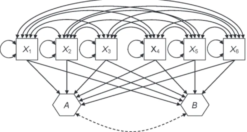
The conceptual difference between PAF and PCA is that factors in PCA are estimated as composites, or weighted linear combinations of the indicators (i.e., total scores). How-ever, factors in PAF have the status of latent variables that are estimated taking account of measurement error. For example, the representation of the two-factor, six-indicator model in Figure 6.2(b) is consistent with the PAF method because common variance is analyzed apart from unique variance, which corresponds to the error terms in the fi gure. Presented in Figure 6.3 is a depiction of a two-factor, six-indicator model analyzed in PCA. The fac-tors in Figure 6.3 are each represented with hexagons, which some authors use in model diagrams to represent composites. The lines with single arrowheads that point from the indicators to the factors represent the fact that factors are estimated as weighted total scores across the indicators in PCA. From this perspective, indicators are the predictors in PCA, but the predictors in PAF are the factors (compare Figure 6.2(b) and Figure 6.3). The dashed line in the symbol for a covariance ( ) in Figure 6.3 represents the possibility for an oblique factor rotation in PCA.
Because the PCA method analyzes observed variables only, some methodologists do not consider it to be a “true” method of factor analysis. Instead, PCA is described by those who hold this view as a mere data reduction technique that replaces a set of correlated variables with a smaller set of orthogonal composites, not as method for estimating latent variables. Others refer to the composites generated in PCA as “components” instead of “factors.” There has been much debate in the literature about the relative merits of PCA versus PAF (e.g., Mulaik, 1992), some of it quite rancorous. It helps to know that PAF and PCA tend to generate similar solutions when scores on all indicators are very reliable, each indicator depends mainly on just one factor, all communalities are relatively high, and the sample size is large (e.g., Velicer & Jackson, 1990). Otherwise, the two methods can generate appreciably different estimates when applied to the same data. Results of PCA and PAF also tend to converge as more and more indicators are analyzed. This hap-pens because the number of diagonal elements as a proportion of all the elements in a data matrix decreases as the number of variables increases (B. Thompson, 2004), and PCA and
Figure 6.3 Conceptual representation of principal components analysis for 6 indicators and 2
PAF analyze the same data matrix except for the diagonal entries. In SPSS, the initial fac-tor solution is extracted using PCA even if the user requested PAF extraction for the fi nal solution. In general, PAF is a better choice than PCA when not all score reliabilities are high (e.g., rXX > .80).
Some other EFA extraction methods are briefl y described next; see Mulaik (2009, chap-ter 7) for more information. The method of alpha factor analysis is a generalization of the internal consistency reliability coeffi cient (i.e., Cronbach’s alpha) but in this case applied to indicators of different factors instead of to items within the same test. This method associates indicators with factors in a way that maximizes the internal consistency of construct measurement. The method of image analysis minimizes the chance that a factor will be defi ned mainly by a single indicator. This outcome is undesirable in factor analy-sis because single-indicator measurement is generally imprecise compared with multiple-indicator measurement. Image analysis works by minimizing the effect of specifi c variance on the results. In maximum likelihood factor analysis, the method of ML estimation is used to derive common factors that reproduce sample correlations among the indicators as close as possible. The method also generates statistical tests of parameter estimates, including the pattern coeffi cients and factor correlations. In contrast, these kinds of sta-tistical tests are not available in the PAF and PCA methods. In SPSS, the ML method is applied to correlation matrices only.
6.6.2 Number of Retained Factors
Sometimes the decision about the number of factors to retain is determined by theory, such as when a cognitive ability test battery is constructed in order to assess three different underlying domains. In this case, it makes sense to specify a three-factor solution. Even when theory indicates a specifi c number of factors, many researchers will nevertheless inspect a range of factor solutions, such as solutions with two, three, or four factors for the example just mentioned. Doing so not only evaluates the original hypothesis about the presence of three factors; it also allows for alternative explanations (i.e., two or four factors) to be tested. There are also various statistical criteria for determining the number of retained factors. It is best not to blindly apply these criteria because doing so tends to capitalize on chance variation in a particular sample. Instead, a researcher should inspect statistical criteria in light of extant theory.
This fi rst statistical criterion is the default basis in most EFA computer procedures for determining the number of retained factors, but this method is not always the best choice. It is the eigenvalue >1.0 rule, also known as the Kaiser criterion or K1 rule after the edu-cational statistician Henry F. Kaiser. Every extracted factor in EFA has its own eigenvalue, which is a measure of the proportion of variance in the indicators explained by that factor and is designated by the symbol λ. The fi rst extracted factor tends to have the highest ei-genvalue, and eigenvalues tend to successively decrease as additional factors are extracted. An eigenvalue is the sum of the squared structure coeffi cients across all the indicators. If λ= 1.0, then the amount of variance explained by that factor corresponds to the amount of information in one indicator, and if λ= 2.0, the explanatory power corresponds to the vari-ability of two indicators, and so. The ratio λ/nj where ni is the number of indicators is the proportion of total variance explained by the associated factor. The sum of the eigenvalues for all possible factors equals the number of indicators, and the ratio of the sum of the eigenvalues across all retained factors divided by the number of indicators is the total pro-portion of variance explained by the factors as a set (B. Thompson, 2004). These propor-tions of explained variance are another type of variance-accounted-for effect size in EFA. The λ1.0 rule thus requires that a factor explains at least one “unit” of information in
terms of the indicators. However, note that the λ1.0 rule applies to factors extracted using the PCA method, not the PAF method. Indeed, it is a mistake to apply this rule when a reduced correlation or covariance matrix is analyzed (Fabrigar et al., 1999).
There are two problems with blindly following the λ1.0 rule. First, sampling error af-fects the estimation of eigenvalues, which ignores that the fact that λ1.01 versus λ.99 leads to categorically different outcomes (i.e., retain vs. do not retain) under this rule. Sec-ond, factor solutions determined by the λ1.0 rule tend to have too many factors but also occasionally too few factors (e.g., Velicer & Jackson, 1990). In general, the λ1.0 rule is not a sound basis for deciding how many factors to retain. A variation is the Cattell scree
test (after the psychologist Raymond B. Cattell), which is a visual heuristic that involves
making a line graph where eigenvalues are plotted on the Y-axis for each of the total pos-sible number of factors, which are represented on the X-axis. The graph is then visually inspected in order to locate the point where the drop in eigenvalues over successive fac-tors levels out and from which the slope of the line is basically horizontal. The number of retained factors in this approach corresponds to the number of eigenvalues before the last substantial drop in the graph. A drawback of the scree test is that its interpretation can be rather subjective in that two different researchers can come to different conclusions after inspecting the same plot.
A more sophisticated method based on eigenvalues is that of parallel analysis, which in-volves the comparison of observed eigenvalues against those expected from random data. One way to conduct a parallel analysis is to use a computer procedure to randomize the scores for each variable in a raw data fi le.2 The randomized scores have the same
distribu-tional characteristics of the original scores, but their expected intercorrelations are about zero. Next, eigenvalues from the analysis of the randomized scores are compared against those from the original data. Factors are retained whenever the eigenvalues based on the original scores are greater than the eigenvalues for the corresponding factors based on the randomized scores. Suppose that the eigenvalues for the fi rst three factors based on ana-lyzing the original scores are, respectively, 5.525, 2.350, and 1.026. The corresponding eigenvalues based on the randomized scores are 2.770, 1.850, and 1.332. This pattern suggests that fi rst two factors should be retained but not the third because 1.332 (based on the randomized scores) is greater than 1.026 (based on the original scores). Results of computer simulation studies about parallel analysis have generally been favorable (e.g., Crawford et al., 2010), but Fabrigar et al. (1999) noted that the decision to retain factors can be rather arbitrary when the pair of eigenvalues for a particular factor are very similar.
Most researchers retain fewer factors than the number of indicators, and such solutions typically explain some proportion of the total variance of the indicators, but usually not all of it. This also means that the factors will not perfectly explain the sample correlations (i.e., the data). Many EFA computer procedures optionally print predicted correlations— also called reproduced correlations—and residual correlations. The former are the values of predicted Pearson correlations for the set of indicators, given the factor solution, and the latter are the differences between the observed and predicted correlations for each indica-tor. The lower the residuals in absolute value, the better the explanatory power of a factor solution. There is no absolute cut-off for interpreting residual correlations, but a better result is indicated if all absolute residuals are < .05. However, absolute residuals >.10 sug-gest poor prediction of the corresponding correlation.
It is generally better in EFA to extract too many factors, or overfactoring, than to retain too few, or underfactoring. This is because there tends to be substantial error in the results with under-factoring. For example, estimation of pattern coeffi cients of indicators that actually depend on a factor may complicate accurate estimation of coeffi cients of other in-dicators that measure retained factors. Two factors that are really distinct may be merged
in a model with too few factors, which may complicate interpretation of the underlying latent variables (Fabrigar et al., 1999). Over-factoring is not without penalty, including the interpretation of factors that do really correspond to hypothetical constructs in the population. Overfactoring is also a potential drawback of the λ1.0 rule.
6.6.3 Method of Rotation
The option for rotation does not apply when only a single factor is retained; otherwise, rotation is part of just about all analyses of multifactor models in EFA. The initial factor solution is often diffi cult to interpret. This is because the structure coeffi cients for the as-sociations between the fi rst factor and all indicators tend to uniformly high, and patterns of correlations with the remaining factors may not be very distinct. The goal of rotation is to make the meaning of the factors more obvious to the researcher. It works by reweight-ing the initial factors (i.e., the factor axes are shifted) accordreweight-ing to statistical criteria that vary with the particular method of rotation. The desired outcome is a rotated solution that exhibits simple structure where each factor explains as much variance as possible in nonoverlapping sets of indicators. That is, the structure coeffi cients for the rotated factors should head toward either 0 or 1.0 in order to make the associations between factors and indicators more distinct. Theoretically, there are an infi nite number of possible factor rota-tions for a given solution. In practice, either the researcher specifi es a rotation option in a computer procedure for EFA or the computer will employ its default method.
There are two main classes of rotation methods in EFA. In orthogonal rotation, the rotated factors are all uncorrelated just as they are in the initial solution. Consequently, values of the standardized pattern coeffi cient and the structure coeffi cient for each indi-cator are equal. The most widely used rotation method of any kind is Kaiser’s varimax
rotation, which is also the default in SPSS. Varimax rotation maximizes the variance of
the structure coeffi cients (i.e., it pushes them toward 0 or 1.0) for each factor, which tends to (a) limit the number of indicators with high correlations with that factor and (b) evenly distribute the indicators across the factors. This method is used so often because it gener-ally yields simple structure in perhaps most EFA studies where the factors are uncorrelated (B. Thompson, 2004). A related method is quartimax rotation, which maximizes the vari-ance of the structure coeffi cients for each indicator. This tends to yield a factor solution with a general factor that correlates highly with most indicators and lesser factors each associated with different subsets of indicators. The method of equamax rotation offers a kind of “comprise” in that it maximizes a weighted function of the criteria from the vari-max method and the quartivari-max method. Selection among these alternatives for orthogo-nal rotation should be guided by the researcher’s hypotheses about the anticipated model. The assumption of all orthogonal rotation methods is that the underlying constructs are uncorrelated, but this hypothesis is not always defensible (Fabrigar et al., 1999). For ex-ample, it makes little sense that various latent cognitive abilities, such as verbal reasoning, visual-spatial reasoning, and memory, would be unrelated to each other. It seems just as implausible to presume that certain latent affective domains, such as anxiety and depres-sion, are independent. Methods of oblique rotation allow the factors to covary; that is, they estimate measurement models with correlated factors. Note that the specifi cation of oblique rotation does not somehow “force” the factors to covary. Instead, these methods estimate factor correlations, given the data, so these estimates are “allowed” to be close to zero, if such estimates are consistent with the data. However, if an estimated factor correlation is extremely high (e.g., ), then the two factors are clearly not distinct (i.e., there are too many factors). Also, the pattern coeffi cients and the structure coeffi cient for the same indicator are typically unequal when the factors covary.
Promax rotation is probably the most widely used oblique rotation method. It usually
begins with a varimax-rotated solution and then raises the pattern coeffi cients to a higher power κ (kappa), which tends to force near-zero coeffi cients to approach zero faster than coeffi cients further from zero (Mulaik, 2009). The procedure then generates least squares estimates of the target matrix just described by allowing the factors to covary. A param-eter of promax rotation is κ, or the power to which coeffi cients in the target matrix are raised. Values of κ usually range from 1 through 4, where higher values permit higher absolute estimates of factor correlations that are consistent with data. The default in SPSS is κ= 4, and it is usually unnecessary to change this value. Another oblique method is
direct oblimin rotation, which is a member of a family of oblimin methods that generally
minimize the variance of the pattern coeffi cients across different factors while estimating factor correlations. The parameter for direct oblimin rotation in SPSS is referred to as
δ (delta), which ranges from negative to positive in value up to a maximum of .80 (i.e.,
δ .80). Lower values of δ tend to decrease absolute estimates of factor correlations and higher values result in just the opposite. The default in SPSS is δ 0, and is rarely necessary to specify a different value.
A potential drawback of oblique rotation is that interpretation of the factors may be more diffi cult. One reason is that there are two sets of standardized coeffi cients, pattern and structure, and it can happen that and their values for the same indicator are quite different. For example, if an indicator’s structure coeffi cient is about zero but its pattern coeffi cient is not, then a suppression effect is indicated. This means that the indicator contributes to the factor indirectly by changing the relations of other indictors to the same factor (B. Thompson, 2004). Another sign of suppression is when the signs of the pattern coeffi cient and structure coeffi cients for the same indicator are different. A second compli-cation of oblique rotation is that there are few guidelines for applied researchers concern-ing the specifi cation of values of parameters for the promax and oblimin methods other than the default values that would be suitable for a particular set of indicators (Costello & Osborne, 2005).
There are many other rotation methods in EFA, and it can be diffi cult to decide which method is best. There is also some degree of trial and error in their use. For example, it could happen in a particular analysis that a promax oblique rotation generates results that are easier to interpret than an oblimin oblique rotation. However, if the results are dramatically different after application of different rotation methods, then there may be little basis to pick one solution or the other when no replication sample is available. How-ever, a robust underlying measurement model with simple structure assessed with psycho-metrically sound indicators should be detected by different rotation methods. See Mulaik (2009, Chapters 10–12) for more information about factor rotation in EFA.
6.6.4 Empirical Example
The fi rst edition of the Kaufman Assessment Battery for Children (KABC-I; Kaufman & Kaufman, 1983) is an individually-administered cognitive ability test for children ages 2½–12½ years old. The test’s authors claimed that the KABC -I’s eight subtests measure two factors. The three tasks believed to refl ect sequential processing all require the correct recall of auditory stimuli (Number Recall, Word Order) or visual stimuli (Hand Move-ments) in a particular order. The other fi ve tasks—Gestalt Closure, Triangles, Spatial Memory, Matrix Analogies, and Photo Series—are supposed to measure more holistic, less order-dependent reasoning, or simultaneous processing. Each of these tasks requires that the child grasps a gestalt but with somewhat different formats and stimuli that all
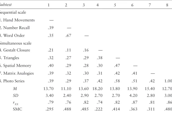
Table 6.1 Input data (correlations, standard deviations, and means) for analysis of a 2-factor model
of the Kaufman Assessment Battery for Children–1st Edition.
Subtest 1 2 3 4 5 6 7 8 Sequential scale 1. Hand Movements — 2. Number Recall .39 — 3. Word Order .35 .67 — Simultaneous scale 4. Gestalt Closure .21 .11 .16 — 5. Triangles .32 .27 .29 .38 — 6. Spatial Memory .40 .29 .28 .30 .47 — 7. Matrix Analogies .39 .32 .30 .31 .42 .41 — 8. Photo Series .39 .29 .37 .42 .58 .51 .42 1.00 M 13.70 11.10 13.60 18.20 13.80 13.90 15.40 12.70 SD 3.40 2.40 2.90 2.70 2.70 4.20 2.80 3.00 rXX .79 .76 .82 .74 .82 .87 .81 .86 SMC .295 .488 .485 .222 .414 .363 .311 .480
Note: SMC = squared multiple correlation. Input data and score reliabilities (split-half coeffi cients) are from
Kaufman and Kaufman (1983), N = 200.
involve visual stimuli.3 The data for this analysis from the test’s standardization sample
for 10-year old children (N = 200) are summarized in Table 6.1. Also reported in the table are score reliability coeffi cients and SMC values for each indicator.
The SPSS syntax listed in Appendix 6.1 submits the summary statistics from Table 6.1 for EFA with the PAF method of factor extraction.4 A two-factor model is specifi ed with
varimax rotation in the fi rst analysis and with promax rotation in the second. The data matrix in both analyses is the correlation matrix of the indicators. Iterative estimation failed in the fi rst attempt to analyze the data because the default limit on the number of iterations (25) was exceeded. The error message generated by SPSS is listed next:
Attempted to extract 2 factors. More than 25 iterations re-quired. Extraction was terminated.
This warning sounds innocuous, but it indicates a serious problem. The number of it-erations was increased to 50 (see Appendix 6.1), and the second run of SPSS terminated normally with a converged and admissible solution.
Listed in the left side of Table 6.2 are the eigenvalues and corresponding percentages of total explained variance for each of the eight factors in the initial solution extracted with PCA of the unreduced correlation matrix. For example, the eigenvalue for the fi rst initial factor is λ1 = 3.536, so this factor accounts for 3.536/8 = .442, or 44.20% of the
variance across all indicators. As expected, the next 7 initial factors explain succes-sively decreasing percentages of variance, and all eight factors together explain a total
Table 6.2 Eigenvalues and percentages of explained variance for analysis of an exploratory 2-factor
model of the Kaufman Assessment Battery for Children–1st Edition.
Factor PCA PAF
Eigenvalue % variance Cumulative % variance
Eigenvalue % variance Cumulative % variance 1 3.536 44.20 44.20 3.045 38.07 38.07 2 1.239 15.49 59.70 .872 10.90 48.97 3 .743 9.29 68.98 4 .649 8.11 77.09 5 .597 7.46 84.56 6 .510 6.38 90.93 7 .416 5.21 96.14 8 .309 3.86 100.00
Note. PCA = principal components analysis; PAF = principal axes factoring. All factors are unrotated.
Figure 6.4 Scree plot for a principal components analysis of Kaufman Assessment Battery for
Children–1st Edition subtests.
of 100% of the variance. A scree plot of the eigenvalues from the initial factors solution is presented in Figure 6.4.
The shape of the plot more or less levels out after extraction of the second factor, which is consistent with the specifi cation of a two-factor model. Values of all absolute residual correlations are < .05, which says that the two-factor model explains the observed cor-relations reasonably well. Because no raw data fi le was available for this analysis, the method of parallel analysis based on randomizing the scores cannot be applied. Reported
in the right side of Table 6.2 are the eigenvalues and percentages of explained variance for the two factors extracted with PAF of the reduced correlation matrix. As expected, the eigenvalues for the two retained factors in the PAF solution are each lower the cor-responding fi rst two factors in the PCA solution. This happens because common vari-ance only is analyzed in PAF, but common varivari-ance is just a fraction of total varivari-ance (see Figure 6.1). Together the fi rst two PAF-extracted factors explain 48.97% of the total variance.
Presented in Table 6.3 are the initial and fi nal communality estimates for each of the eight indicators from the PAF results. Note in Table 6.3 that the initial estimate for each indicator equals the SMC of that indicator with all others in the sample (see Table 6.1). The fi nal set of communality estimates in Table 6.3 is from converged iterative estima-tion. The fi nal estimate is also greater than the initial estimate for each indicator. For example, the initial communality estimate for the Number Recall task is .488, but the fi nal estimate is .865 (Table 6.3). This pattern is expected because sample SMC values are generally attenuated by measurement error, but iterative estimation account for this effect.
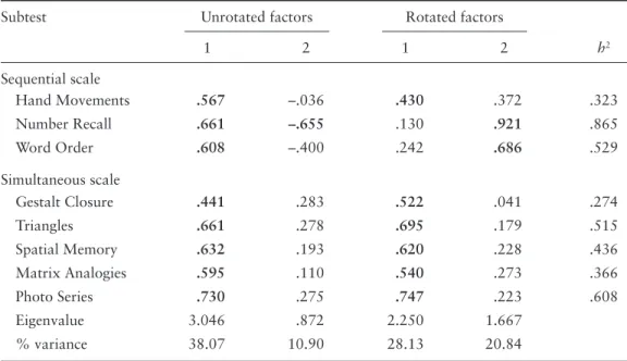
Standardized pattern coeffi cients for all eight indicators across the 2 unrotated factors and across the 2 varimax-rotated factors from the PAF results are listed in Table 6.4. Be-cause each pair of factors is orthogonal, the standardized pattern coeffi cients in the table are also structure coeffi cients. Observe in Table 6.4 that (a) the sum of the squared struc-ture coeffi cients for each indicator across both factors in the each of the unrotated and ro-tated solutions equals the fi nal communality estimate for that indicator. Also, (b) the sum of the squared structure coeffi cients for each factor equals the eigenvalue for that factor, within slight rounding error. (Readers should verify these statements.) There is no single standard for interpreting the magnitudes of structures coeffi cients in EFA, but one rule of thumb is that absolute structure coeffi cients > .40 indicate appreciable indicator-factor cor-respondence (e.g., Thompson, 2004). Accordingly, absolute coeffi cients > .40 in Table 6.4 are listed in boldface. It is no surprise in the unrotated solution that all eight indicators have relatively high correlations with the fi rst extracted factor. However, the pattern of structure coeffi cients across the 2 varimax-rotated factors is more distinct. For example, all 5 subtests of the KABC-I’s Simultaneous Processing scale correlate appreciably with the
Table 6.3 Communality estimates for subtests of the Kaufman Assessment Battery for Children–1st
Edition.
Subtest Initial Final
Sequential scale Hand Movements .295 .323 Number Recall .488 .865 Word Order .485 .529 Simultaneous scale Gestalt Closure .222 .274 Triangles .414 .515 Spatial Memory .363 .436 Matrix Analogies .311 .366 Photo Series .480 .608
fi rst rotated factor (see Table 6.4). Two of three subtests on the Sequential Processing scale have their highest correlations with the second rotated factor, but the other task, Hand Movements, correlates higher with the fi rst rotated factor than the second. Thus, this task from the Sequential Processing scale seems to have more common with those from the Simultaneous Processing scale.
The assumption that cognitive ability factors are uncorrelated may be implausible. Thus, a second analysis using PAF extraction of 2 factors was conducted with the cor-relations in Table 6.1 but now with promax rotation. The estimated factor correlation in this analysis is .503, which says that the two factors share about 25% of their variance in common. Because the factors are correlated in this analysis, the standardized pattern coeffi cients are not also structure coeffi cients. Both sets of coeffi cients just mentioned are reported in Table 6.5 for each indicator.
The same general pattern of indicator-factor correspondence suggested by the struc-ture coeffi cients from oblique rotation is similar to that suggested by the coeffi cients from orthogonal rotation (compare entries in the right sides of, respectively, Table 6.4 and Table 6.5). The results from oblique rotation in Table 6.5 also indicate suppression effects for some indicators. For example, the standardized pattern coeffi cient for predict-ing the Number Recall task from the from the fi rst promax-rotated factor is negative (–.11), but the correlation between this indicator and the fi rst factor is positive (.38). Suppression effects are also apparent for the Gestalt Closure task and the Triangles task (see Table 6.5). Overall, the EFA results are consistent with a two-factor model, but the Hand Movements task of the Sequential Processing scale is problematic because it seems to belong more with the tasks on the Simultaneous Processing scale. Results of CFA for these data described in the next section yield even more precise results concerning this particular indicator.
Table 6.4 Standardized pattern coeffi cients for unrotated and varimax-rotated factors of the
Kaufman Assessment Battery for Children.
Subtest Unrotated factors Rotated factors
1 2 1 2 h2 Sequential scale Hand Movements .567 –.036 .430 .372 .323 Number Recall .661 –.655 .130 .921 .865 Word Order .608 –.400 .242 .686 .529 Simultaneous scale Gestalt Closure .441 .283 .522 .041 .274 Triangles .661 .278 .695 .179 .515 Spatial Memory .632 .193 .620 .228 .436 Matrix Analogies .595 .110 .540 .273 .366 Photo Series .730 .275 .747 .223 .608 Eigenvalue 3.046 .872 2.250 1.667 % variance 38.07 10.90 28.13 20.84
Note: h2, fi nal communality estimate. All coeffi cients are also structure coeffi cients. Absolute coeffi cients .40
6.7 Confi rmatory Factor Analysis
As in EFA, the decision sequence for CFA begins with construct defi nition, indicator selec-tion, and a sampling plan. Before collecting the data, the researcher should also specify the restricted measurement model to be analyzed in CFA and then check whether it is identifi ed. The former requires specifi cation of the number of factors in the model and the pattern of indicator-factor correspondence. The hypothesis of unidimensional measure-ment requires that there is a single pattern coeffi cient for each indicator and that there are no correlated errors (e.g., Figure 6.2(b)), that is, the model is a standard CFA model. Most CFA models described in the literature are standard models. Specifi cation of multidimen-sional measurement is an option, but doing so requires a substantive rationale in order to allow indicators to depend on more than one factor or the specifi cation of error correla-tion between a pair of indicators. Such nonstandard CFA models are more complex than standard models, and they are not always identifi ed, an issue considered next.
6.7.1 Identifi cation Requirements
A CFA measurement model is identifi ed if it is theoretically possible for the computer to derive a unique estimate of every model parameter. The word “theoretically” emphasizes identifi cation as a property of the model and not of the data. For example, if a model is not identifi ed, then it remains so regardless of the sample size (N = 100, 1,000, etc.). Therefore, models that are not identifi ed must be respecifi ed; otherwise, attempts to an-alyze them may be fruitless. There are two necessary but insuffi cient requirements for identifi cation: (1) Every factor and error term must be assigned a scale, and (2) the model
degrees of freedom must be at least zero (dfM 0) The fi rst requirement just mentioned
was discussed earlier and is represented in diagrams of CFA models with the scaling con-stant “1” (e.g., Figure 6.2(b)).
The quantity dfM is the difference between the number of observations available in the
analysis and the number of model parameters, which in CFA are the pattern coeffi cients,
Table 6.5 Standardized coeffi cients for promax-rotated factors of the Kaufman Assessment Battery
for Children–1st Edition.
Subtest Pattern coeffi cients Structure coeffi cients
Factor 1 Factor 2 Factor 1 Factor 2
Sequential scale Hand Movements .379 .274 .517 .464 Number Recall –.111 .981 .383 .925 Word Order .081 .684 .424 .724 Simultaneous scale Gestalt Closure .575 –.123 .513 .166 Triangles .730 –.026 .717 .341 Spatial Memory .632 .053 .659 .371 Matrix Analogies .531 .128 .595 .395 Photo Series .777 .005 .780 .396