The Evolution of the Galaxy Stellar Mass Function at z = 4-8: A Steepening Low-mass-end Slope with Increasing Redshift

Preprint typeset using LA_{TEX style emulateapj v. 12/16/11}

THE EVOLUTION OF THE GALAXY STELLAR MASS FUNCTION ATz= 4–8: A STEEPENING LOW-MASS-END SLOPE WITH INCREASING REDSHIFT

Mimi Song1_{, Steven L. Finkelstein}1_{, Matthew L. N. Ashby}2_{, A. Grazian}3_{, Yu Lu}4_{, Casey Papovich}5_{, Brett}

Salmon5, Rachel S. Somerville6, Mark Dickinson7, K. Duncan8,9, Sandy M. Faber10, Giovanni G. Fazio2, Henry C. Ferguson11, Adriano Fontana3, Yicheng Guo10, Nimish Hathi12, Seong-Kook Lee13, Emiliano Merlin3, S. P.

Willner2

Submitted to the ApJ

ABSTRACT

We present galaxy stellar mass functions (GSMFs) atz= 4–8 from a rest-frame ultraviolet (UV) selected sample of ∼4,500 galaxies, found via photometric redshifts over an area of∼280 arcmin2_in

the CANDELS/GOODS fields and the Hubble Ultra Deep Field. The deepest Spitzer Space Tele-scope/IRAC data yet-to-date from the Spitzer-CANDELS (26.5 mag, 3σ) and the IRAC Ultra Deep Field 2010 (26.4–27.1 mag, 3σ) surveys allow us to place robust constraints on the low-mass-end slope of the GSMFs, while the relatively large volume provides a better constraint at higher masses compared to previous space-based studies. Supplemented by a stacking analysis, we find a linear correlation between the rest-frame UV absolute magnitude at 1500˚A (MUV) and logarithmic stellar

mass (logM∗). We use simulations to validate our method of measuring the slope of the logM∗–MUV

relation, finding that the bias is minimized with a hybrid technique combining photometry of indi-vidual bright galaxies with stacked photometry for faint galaxies. The resultant measured slopes do not significantly evolve over z= 4–8, while the normalization of the trend exhibits a weak evolution towards lower masses at higher redshift for galaxies at fixed MUV. We combine the logM∗–MUV

distribution with observed rest-frame UV luminosity functions at each redshift to derive the GSMFs. While we see no evidence of an evolution in the characteristic massM∗_{, we find that the low-mass-end} slope becomes steeper with increasing redshift from α = −1.53+0₋0..0706 at z= 4 to α= −2.45+0−0..3429 at

z = 8. The inferred stellar mass density, when integrated over M∗ = 108–1013 M, increases by a factor of 13+35₋9 betweenz= 7 andz= 4 and is in good agreement with the time integral of the cosmic

star-formation rate density.

Subject headings: galaxies: evolution — galaxies: formation — galaxies: high-redshift — galaxies: mass function

1. INTRODUCTION

The near-infrared (near-IR) capability of the Wide Field Camera 3 (WFC3) on-board theHubble Space Tele-scope (HST) has now yielded a statistically significant

[email protected]

1_{Department of Astronomy, The University of Texas at} Austin, C1400, Austin, TX 78712, USA

2_{Harvard-Smithsonian Center for Astrophysics, 60 Garden} St., Cambridge, MA 02138, USA

3_{INAF – Osservatorio Astronomico di Roma, via Frascati 33,} 00040 Monteporzio, Italy

4_{Observatories, Carnegie Institution for Science, Pasadena,} CA, 91101

5_{Department of Physics and Astronomy, Texas A&M} Univer-sity, College Station, TX 77843, USA

6_{Department of Physics & Astronomy, Rutgers University,} 136 Frelinghuysen Road, Piscataway, NJ 08854

7_{National Optical Astronomy Observatory, Tucson, AZ 85719} 8_{University of Nottingham, School of Physics & Astronomy,} Nottingham NG7 2RD

9_{University of California Observatories/Lick Observatory,} University of California, Santa Cruz, CA, 95064

10_{Leiden Observatory, Leiden University, NL-2300 RA} Lei-den, The Netherlands

11_{Space Telescope Science Institute, Baltimore, MD 21218} 12_{Aix Marseille Universite, CNRS, LAM (Laboratoire} d’Astrophysique de Marseille) UMR 7326, 13388, Marseille, France

13_{Center for the Exploration of the Origin of the Universe} (CEOU), Astronomy Program, Department of Physics and As-tronomy, Seoul National University, Shillim-Dong, Kwanak-Gu, Seoul 151-742, Korea

sample of galaxies in the early universe, enabling us to pass the era of simply discovering very distant galaxies, and enter an era where we can perform systematic studies to probe the underlying physical processes. Such stud-ies have begun to make progress towards understand-ing galaxy evolution at high redshift, with particular ad-vances in measurements the rest-frame ultraviolet (UV) luminosity function (e.g., Bouwens et al. 2011; Oesch et al. 2012; Schenker et al. 2013b; Lorenzoni et al. 2013; Finkelstein et al. 2015; Bouwens et al. 2015), the rest-frame UV spectral slope (e.g., Finkelstein et al. 2012; Bouwens et al. 2014), and the cosmic star formation rate density (SFRD; see Madau & Dickinson 2014 for a re-view).

A key constraint on galaxy evolution which has only re-cently begun to be robustly explored is that of the growth of stellar mass in the universe. This measurement re-quires a combination of deepHSTdata with constraints at rest-frame optical wavelengths, to better probe the emission from older, lower-mass stars. The mass assem-bly history across cosmic time is governed by complicated processes, including star formation, merging of galaxies, supernovae feedback, etc. In spite of the complexity of the baryonic physics of galaxy formation, however, var-ious studies have found that global galaxy properties, such as star formation rate, metallicity, size, etc., all cor-relate tightly with the stellar mass (Kauffmann et al.

2003b; Noeske et al. 2007; Tremonti et al. 2004; Williams et al. 2010), implying that the stellar mass plays a major role in galaxy evolution. Thus, determining the comov-ing number density of galaxies in a wide range of stellar masses (i.e., the galaxy stellar mass function) and follow-ing the evolution with redshift constitutes a basic and crucial constraint on galaxy formation models. Specifi-cally, obtaining robust observational constraints on the low-mass-end slope of the GSMF can provide insights on the impact of feedback on stellar mass build-up of low mass galaxies (Lu et al. 2014), as current theoretical models predict steeper low-mass-end slopes than those previously observed (e.g., Vogelsberger et al. 2013; see Somerville & Dav´e 2014 for a review). Consequently, the evolution of GSMFs over the past 11 billion years has been extensively investigated observationally during the past decade (e.g., Marchesini et al. 2009; Baldry et al. 2012; Ilbert et al. 2013; Muzzin et al. 2013; Tomczak et al. 2014), mostly using traditional techniques (e.g., 1/Vmax, maximal Likelihood) which assess and correct

for the incompleteness in mass.

Nonetheless, the GSMF in the first two billion years after the Big Bang has remained poorly constrained, due toi) limited sample sizes, particularly of low-mass galax-ies at high redshift,ii) systematic uncertainties in stellar mass estimations, andiii) the lack ofSpitzer Space Tele-scopeInfrared Array Camera (IRAC; Fazio et al. 2004) data with comparable depth toHST/WFC3. IRAC data are essential to probe stellar masses of galaxies atz&4 as the 4000 ˚A/Balmer break moves into the mid-infrared (mid-IR), beyond the reach of HST (and ground-based telescopes).

An alternative approach to deriving the GSMF takes advantage of the fact that the selection effects and in-completeness are relatively well known and corrected for in rest-frame UV luminosity functions. Therefore, one can derive GSMFs by taking a UV luminosity function and convolving it with a stellar mass versus UV lumi-nosity distribution at each redshift. Using this approach, Gonz´alez et al. (2011) derived GSMFs at 4< z < 7 of Lyman-break galaxies (LBGs) over∼33 arcmin2 _{of the}

Early Release Science (ERS) field (forz= 4–6, and the Hubble Ultra Deep Field (HUDF) and the Great Obser-vatories Origins Deep Survey (GOODS) fields with pre-WFC3 data for z = 7) utilising the HST/WFC3 and IRAC GOODS-South data. They reported a shallow low-mass-end slope of −(1.4–1.6) at z = 4–7, but the small sample size and limited dynamic range made it difficult for them to explore the mass-to-light distribu-tion atz >4, and their GSMFs were derived under an assumption that the mass-to-light distribution at z∼4 is valid up toz∼7.

More recently, several studies have utilised the large

HST dataset from the Cosmic Assembly Near-infrared Deep Extragalactic Legacy Survey (CANDELS; Grogin et al. 2011; Koekemoer et al. 2011) to make progress on the measurements of the GSMFs at z > 4. Dun-can et al. (2014) and Grazian et al. (2015) derived the GSMFs of galaxies at 4 < z < 7 in the GOODS-S field and GOODS-S/UDS fields, respectively, using the CANDELS HST data and the Spitzer Extended Deep Survey (SEDS; Ashby et al. 2013) IRAC data. These studies have reported a steeper low-mass-end slope of

α ∼ −(1.6–2.0) than previous studies, but the uncer-tainties are still large, and the inferred evolution of the low-mass-end slope of the GSMFs remains uncertain.

Here we probe galaxy build-up from z = 4 out to

z = 8, aiming to improve on the limiting factors dis-cussed above, with a goal of providing robust constraints on the GSMFs of galaxies at 4 < z < 8. We do this by combining near-IR data from CANDELS GOODS-S and GOODGOODS-S-N fields with the deepest existing IRAC data over the GOODS fields from theSpitzer-CANDELS (S-CANDELS; PI Fazio; Ashby et al. 2015) and the IRAC Ultra Deep Field 2010 Survey (UDF10; Labb´e et al. 2013). We obtain reliable photometry on these deep IRAC data by performing point-spread function (PSF)-matched deblending photometry, enabling us to extend the exploration of the GSMFs to lower stellar masses and higher redshifts than previous studies. Furthermore, a special emphasis is put on quantifying and minimizing the systematics inherent in our analysis via mock galaxy simulations. While taking a similar approach of convolv-ing a rest-frame UV luminosity function with stellar mass to rest-frame UV luminosity distribution as Gonz´alez et al. (2011), the increased sample size and deeper data en-able us to bypass the limitations of the previous studies, as we measure the mass-to-light ratio distribution at ev-ery redshift.

This paper is organized as follows. Section 2 intro-duces the HST datasets used in this study as well as our sample at 3.5 < z < 8.5 selected by photometric redshifts and discusses our IRAC photometry, which is critical for the stellar mass estimation described in Sec-tion 3. SecSec-tion 4 presents stellar mass versus observed rest-frame absolute UV magnitude (M∗–MUV)

distribu-tions and introduces a stacking analysis and mock galaxy simulations. By combining the rest-frame UV luminos-ity function with the M∗–MUV distribution, we derive

GSMFs and stellar mass densities in Section 5 and 6, respectively. A discussion and summary of our results follow in Section 7 and Section 8. Throughout the pa-per, we use the AB magnitude system (Oke & Gunn 1983) and a Salpeter (1955) initial mass function (IMF) between 0.1 M and 100 M. All quoted uncertainties represent 68% confidence intervals unless otherwise spec-ified. We adopt a concordance ΛCDM cosmology with

H0 = 70 = 100h km s−1 Mpc−1, ΩM = 0.3, and ΩΛ =

0.7. The HST bands F435W, F606W, F775W, F814W, F850LP, F098M, F105W, F125W, F140W, and F160W will be referred as B, V, i, I814, z, Y098, Y, J, JH140,

and H, respectively.

2. DATA

Constraining GSMFs requires a deep multi-wavelength dataset over a wide area in order to probe the full dy-namic range of a galaxy population. In this section, we describe theHSTimaging used to select our galaxy can-didates, as well as the candidate selection process. We then discuss the procedures used to measure accurate photometry for these galaxies from theSpitzer/IRAC S-CANDELS imaging.

2.1. HST Data and Sample Selection

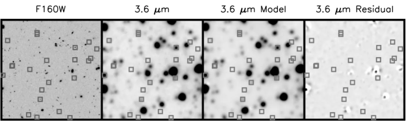
Fig. 1.— Example of our IRAC photometry modeling procedure. Fromlefttoright: 1)H-band WFC3 imaging of a 10_×10_{region in the} GOODS-S field, 2) S-CANDELS 3.6µm imaging, 3) the best-fit 3.6µm model image, and 4) thet-photresidual image (i.e., real science image subtracted by the best-fit model image). Our high-redshift galaxies (grey squares) are often blended with nearby foreground sources, therefore we perform PSF-matched photometry on the S-CANDELS data using the WFC3H-band imaging as a prior on the position and morphology of sources. Using thet-photsoftware package, we convolve theH-band image with empirically-derived IRAC PSFs to generate low-resolution (IRAC) model images, allowing the flux of each source to vary to simultaneously fit all sources in the IRAC data.

for full details of theHSTdata used and the galaxy sam-ple selection. This samsam-ple consists of ∼7,000 galaxies selected via photometric redshifts over a redshift range ofz= 3.5–8.5. These galaxies were selected usingHST

imaging data from the CANDELS (Grogin et al. 2011; Koekemoer et al. 2011) over the GOODS (Giavalisco et al. 2004) North (GOODS-N) and South (GOODS-S) fields, the ERS (Windhorst et al. 2011) field, and the HUDF (Beckwith et al. 2006; Bouwens et al. 2010; Ellis et al. 2013) and its two parallel fields (Oesch et al. 2007; Bouwens et al. 2011).14 _{We use the full dataset which}

in-corporates all earlier imaging fromHSTAdvanced Cam-era for Surveys (ACS), including the B, V, i, I814, and

z filters. We also use imaging from the HST WFC3 in the Y098, Y, J, JH140, and H filters. A complete de-scription of these data is presented by Koekemoer et al. (2011, 2013). These combined data are three-layered in depth, comprising the extremely deep HUDF, moder-ately deep CANDELS-Deep fields, and relatively shallow CANDELS-Wide and ERS fields, designed to efficiently sample both bright and faint galaxies at high redshifts.

As described by Finkelstein et al. (2015), sources were detected in a summedJ+H image, using a more aggre-sive detection scheme compared to that used to build the official CANDELS catalog (e.g., Guo et al. 2013, Barro et al. in prep.) to detect faint sources at high redshifts, yielding a catalog with the total number of sources a factor of two larger. To minimize the presence of spuri-ous sources, only those objects with≥ 3.5σ significance in both the J and H bands were evaluated as possible high-redshift galaxies. Photometric redshifts were esti-mated with EAZY (Brammer et al. 2008), and selection criteria devised based on the full redshift probability dis-tribution function (P(z)) were applied (Finkelstein et al. 2015). A comparison of our photometric redshifts for galaxies with spectroscopic redshifts shows an excellent agreement, withσ(∆z/(1 +zspec)) = 0.03 (after 3σ

clip-ping). All of the selected sources were visually inspected for removal of artifacts and stellar contaminants. Ac-tive galactic nuclei (AGNs) identified in X-rays were also

14 _{Finkelstein et al. (2015) also include about 500 more galaxies} from the Abell 2744 and MACS J0416.1-2403 parallel fields from the Hubble Frontier Fields dataset, while we do not, reducing our full sample to∼7,000 galaxies.

excluded from the sample. Our final parent sample con-sists of 4156, 2056, 669, 284, and 77 galaxies at z = 4 (3.5 < z <4.5), 5 (4.5< z <5.5), 6 (5.5< z <6.5), 7 (6.5< z <7.5), and 8 (7.5< z <8.5), respectively.

2.2. IRAC Data and Photometry

At 3.5 < z < 8.5, the observed mid-IR probes rest-frame optical wavelengths redward of the Balmer/4000 ˚A break. Deep Spitzer/IRAC data are therefore critical to constrain stellar masses and the resulting GSMF. One of the key advances of our study is the significantly in-creased depth in the 3.6 and 4.5µm IRAC bands pro-vided by the new S-CANDELS survey (Ashby et al. 2015). The final S-CANDELS mosaics in the GOODS-S and GOODGOODS-S-N fields (where the former includes the HUDF parallel fields) include data from three previous studies: GOODS, with integration time of 23–46 hr per pointing (Dickinson et al., in preparation); a 50×50region in the ERS observed to 100 hr depth (PI Fazio); and the IRAC Ultra Deep Field 2010 program, which observed the HUDF and its two parallel fields to 120, 50, and 100 hr, respectively (Labb´e et al. 2013). The total integra-tion time within the S-CANDELS fields more than dou-bles the integration time for most of the area used in this study (to≥50 hr total), reaching a total formal depth of 26.5 mag (3σ) at 3.6µm and 4.5µm (Ashby et al. 2015). Imaging at 5.8 and 8.0 µm were obtained with IRAC as part of the GOODS program. However, these data are too shallow to provide meaningful constraints for high-redshift faint galaxies, so we do not include them in our analysis.

The full-width at half-maximum (FWHM) of the PSF of the IRAC data (∼1.700_{at 3.6 µm versus∼0.19}00_{at 1.6}

photom-etry uses information in a high resolution image (here theH-band), such as position and morphology, as priors. Specifically, we use isophotes and light profiles from the detection (J+H) image obtained by the Source Extractor package (SExtractor; Bertin & Arnouts 1996). The high resolution image was convolved with a transfer kernel to generate model images for the low-resolution data (here the IRAC imaging) allowing the flux in each source to vary. This model image was in turn fitted to the real low-resolution image. The IRAC fluxes of sources are determined by the model which best-represents the real data.

As the PSF FWHM of the high-resolution image (H -band) is negligible (∼0.1900_{) when compared to those of} the low-resolution IRAC images (∼1.700_{), we used IRAC} PSFs as transfer kernels. We derive empirical PSFs in each band and in each field by stacking isolated and mod-erately bright ([3.6],[4.5]=15.5–19.0 mag) stars identified in a half-light radius versus magnitude diagram in IRAC imaging. Ast-photrequires the kernel to be in the pixel scale of the high-resolution image, each star image was 10 times oversampled to generate the final PSFs in the same pixel scale of theH-band image (0.0600_{/pixel). They} were then registered, normalized, and median combined to generate the final IRAC PSFs.

Preparatory work for running t-phot includes per-forming background subtraction on the S-CANDELS mosaics using a scriptsubtract bkgd.py(written by H. Ferguson; see Galametz et al. 2013 for details) and di-lation of theJ+HSExtractor segmentation map, analo-gous to the traditional aperture correction. The need for this dilation step originates from the fact that under non-zero background fluctuations, isophotes of faint sources include a smaller fraction of their total flux compared to bright sources, and therefore their IRAC fluxes based on isophotes tend to be underestimated. To include the light in the wings and to counterbalance the underestimation of flux for faint sources of which the amount depends on the isophotal area, an empirical correction factor to en-large the SExtractor segmentation map was devised by the CANDELS team by comparing isophotal area from deep and shallow images (see Galametz et al. 2013 and Guo et al. 2013 for details). We applied this empirical correction factor to theJ+Hsegmentaion map using the programdilate(De Santis et al. 2007) while preventing merging between sources.

To correct for potential small spatial distortions or mis-registrations between the high-resolution and low-resolution images, a second run oft-photwas performed using a shifted kernel built by cross-correlating the model and real low-resolution images. Figure 1 presents an example of our IRAC photometry procedure on a sub-region in GOODS-S. With the exception of very bright sources, the residual image is remarkably clean, high-lighting the accuracy of this procedure.

2.2.1. Verification

We tested the accuracy of our IRAC photometry in two ways. First, we compared our catalog with the of-ficial CANDELS catalogs (Guo et al. 2013; Barro et al. in prep) in which IRAC fluxes were obtained from the shallower SEDS data usingTFIT. As shown in Figure 2, the comparison between our magnitude and that from the official catalog for sources with signal-to-noise ratio

-2

-1

0

1

2

_3.6

µ

m

18

20

22

24

26

28

mag (TPHOT S-CANDELS)

-2

-1

0

1

2

_4.5

µ

m

mag(TPHOT S-CANDELS) - mag(TFIT SEDS)

Fig. 2.— A comparison between ourt-photS-CANDELS pho-tometry and the official CANDELSTFITSEDS photometry from Guo et al. (2013) and Barro et al. (in prep.) for IRAC 3.6µm (upper) and 4.5µm (lower) bands for sources with S/N >1 in both catalogs. Blue circles and error bars indicate the median and robust standard deviation of the magnitude difference in each magnitude bin, and the blue dashed lines encompass the central 68% of the distribution. The red vertical dotted line denotes the 5σS-CANDELS depth. The SEDS data are shallower, thus the agreement between the two catalogs indicates our photometry is accurate. The bias seen at faint magnitudes is due to Eddington bias of up-scattered sources in the shallower SEDS data.

(S/N) greater than unity (S/N>1) in both catalogs in-dicates an excellent agreement with a negligible system-atic offset down to ∼26 mag (3σ depth for the official CANDELS catalog). Fainter sources are dominated by background fluctuations and the Eddington bias of up-scattered sources in the shallower SEDS data, making the comparison unreliable (see Figure 13 of Guo et al. for a similar trend and discussion of the flux comparison).

There--4

-2

0

2

4

3.6

µ

m

20

22

24

26

28

mag (IN)

-4

-2

0

2

4

4.5

µ

m

11 10 01 00

11 10 01 00

mag (IN) - mag (OUT)

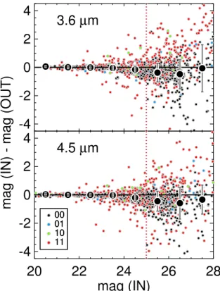
Fig. 3.— Comparison between the input and recovered IRAC 3.6µm (upper) and 4.5µm (lower) magnitude in our mock source simulations. Symbols are color-coded by blendedness in the two filters (shown in the inset in binary notation)—00: contamination-free, 01: contaminated in 4.5 µm, 10: contaminated in 3.6µm, 11: contaminated in both 3.6 and 4.5 µm. Large black circles and error bars represent the median and standard deviation of the magnitude difference of confusion-free sources (small black circles) in each magnitude bin, demonstrating the reliability of our IRAC photometry down to the 50% completeness limit of 25 mag (red vertical dotted line; Ashby et al. 2015).

fore, our simulation results should not be sensitive to those assumptions in the first order. These mock sources were convolved with the PSF of each filter and added at random locations in the (H-band PSF-convolved) high-resolution and IRAC low-high-resolution images. Our simula-tion thus account fully for source confusion with nearby foreground real sources, but we constrain the number density of mock sources to be negligible (5 arcmin−2₎

compared to that of real sources to ensure that our simu-lation results are not dominated by self-crowding among the inserted artificial sources. The mock sources were then recovered using the same procedures as for real sources, includingt-photphotometry. Figure 3 shows a comparison between the input and recovered 3.6µm and 4.5 µm magnitudes. It is encouraging that we find no systematic offset between the two down to the 50% com-pleteness limit of 25 mag (Ashby et al. 2015), given that the IRAC photometry is affected with many sources of uncertainty which demand accurate background subtrac-tion, aperture correction scheme (dilation), and build-up of transfer kernels. As any observed offsets from these simulations are not statistically significant, we do not apply any correction to our observed IRAC photometry.

2.2.2. Visual inspection

A practical limitation exists when building empirical IRAC PSFs for deep fields, as such surveys by design target a relatively small area well off the Galactic plane, resulting in few stars present in the imaging. The se-vere source confusion in the IRAC data further reduces the number of isolated stars which can be used for the creation of PSFs. Therefore, although our PSF-matched IRAC photometry significantly improves photometric ac-curacy over more traditional methods (Lee et al. 2012), our IRAC photometry may be imperfect. Its significance, however, is likely small as already discussed in the pre-vious sections.

Another source of uncertainty is thatTFIT/TPHOT as-sumes no morphologicalk-corrections (no variation in the surface profile or morphology) between short and long wavelength images, which is likely not the case (although we attempted to mitigate this by using the reddestHST

image as our resolution image). However, our high-redshift galaxies are small enough to not be resolved in the low-resolution image (see Figure 25 of Ashby et al. 2013), and thus it should have a negligible effect on the derived fluxes. Bright (and extended) foreground sources in close proximity to our high-redshift sample, however, are prone to imperfect modeling in this case (even with perfect PSFs) and leave residuals which in turn can sig-nificantly affect the photometry of faint sources nearby.

To account for these uncertainties, we visually in-spected the IRAC science and residual images of all ∼7,000 sources in our sample to ensure their IRAC pho-tometry is reliable. Sources falling on strong residuals from nearby bright sources often have recovered signal-to-noise (S/N) ratios which are too high (even when we cannot visually identify counterparts in the IRAC im-ages) or significantly negative, which indicates their pho-tometry is not reliable in general. This is confirmed by a mock source simulation in which we added mock sources at various positions around a bright source, finding that the recovered flux is highly biased (either overestimated or underestimated depending on the “yin” and “yang” of the residual on which the mock source was inserted). We therefore caution against blindly taking IRAC fluxes from a catalog and stress the importance of visual in-spection of IRAC images and residuals of all objects, as contaminated sources can significantly impact studies on individual galaxies or with small number statistics (e.g., the high-mass end of the GSMF).

Contaminated sources are excluded from the sample in our subsequent analysis. This leaves ∼63, 63, 54, 61, 57% of our z = 4,5,6,7,8 parent sample free from a possible contamination from nearby bright sources,15

resulting in 2611, 1292, 364, 172, 44 sources in our fi-nal z = 4,5,6,7,8 selection. Among the final sample, 1172/2611, 480/1292, 108/364, 41/172, 6/44 (45, 37, 30, 24, 14%) sources at z = 4,5,6,7,8, respectively, have

& 2σ detections at 3.6 µm, and 613/2611, 211/1292, 43/364, 12/172, 1/44 (23, 16, 12, 7, 2%) show S/N >

5. A final multi-wavelength catalog was constructed by combining theHSTcatalog and the IRACt-phot cata-log for this final sample.

3. STELLAR POPULATION MODELING

We derived stellar masses and rest-frame UV luminosi-ties for our sample galaxies by fitting the observed spec-tral energy distribution (SED) from the B, V, i, I850, z, Y098, Y, J, JH140, H, 3.6 µm, and 4.5 µm data to the Bruzual & Charlot (2003) SPS models. We refer the reader to Finkelstein et al. (2012, 2015) for a de-tailed explanation of our modeling process. Briefly, we modeled star formation histories as exponentially declin-ing (τ = 1 Myr–10 Gyr), constant (τ = 100 Gyr), and rising (τ = −300 Myr, −1 Gyr, −10 Gyr). Allowable ages spanned a lower age limit of 1 Myr to the age of the universe at the redshift of a galaxy, spaced semi-logarithmically, and metallicity ranged from 0.02 to 1

Z. We assumed the Calzetti et al. (2000) attenuation cuve with E(B −V) = 0.0–0.8 (AV = 0.0–3.2), and

IGM attenuation was applied using the Madau (1995) prescription. All the models were normalized to a total mass of 1M.

One of the major sources of uncertainty in stellar mass measurements of high-redshift galaxies derived from broadband imaging data via SED fitting is the con-tribution of nebular emission. Spectroscopically measur-ing the contribution of strong emission lines (e.g., Hα, [Oiii]λλ4959,5007) to the broadband fluxes for z & 4 galaxies is not currently feasible because they redshift into the mid-IR. Many efforts, however, have been put taking an alternative approach of investigating IRAC col-ors of spectroscopically confirmed galaxies at the redshift range such that only one of the first two IRAC bands is expected to be contaminated by a strong emission line (e.g., Shim et al. 2011; Stark et al. 2013). Together with an inference from the direct measurements of nebular lines of galaxies at lower-redshift (e.g., z ∼3; Schenker et al. 2013a), several studies claim that the contribution of nebular emission to the broadband fluxes for galaxies at high redshift, and thus to the inferred stellar mass, can be significant (e.g., Schaerer & de Barros 2010).

While a more concrete answer on the nebular contribu-tion will need to wait for the advent of theJames Webb Space Telescope(JWST), we took into account the con-tribution of nebular emission in our SED modeling in a self-consistent way following the prescription of Salmon et al. (2015). In this prescription, the strengths of H and He recombination lines (including Hβ) are set by the number of non-escaping ionizing photons, and the strengths of metal lines relative to Hβ are given by In-oue (2011). The nebular line strengths are thus a func-tion of the populafunc-tion age and metallicity (which sets the number of ionizing photons), as well as the ionizing photon escape fraction. We added the nebular lines to the stellar continuum assuming an escape fraction of zero and no extra dust attenuation for nebular emission (i.e.,

E(B−V)stellar=E(B−V)nebular). Figure 4 presents a

comparison of the inferred equivalent width (EW) distri-bution of [Oiii]λλ4959,5007 from our SED modeling for spectroscopically confirmed galaxies at 3.5 < z < 4.5 with the observed EW([Oiii]) histogram of 20 LBGs at similar redshifts (3.0 < z < 3.8) in Schenker et al. (2013a), showing a good agreement.

Our final stellar+nebular line stellar population mod-els are integrated through all of the filter bandpasses in our photometry catalog. The best-fit model for each

0

1

2

3

4

log (EW([OIII])/ )

0

5

10

15

N

This study

Schenker+13 (3.0 < z < 3.8)

Fig. 4.— A comparison of the inferred rest-frame EW([Oiii]λλ4959,5007) distrbution derived from our SED fitting analysis for galaxies in ourz∼4 sample with spectroscopic red-shifts (black solid histogram) with the spectroscopic EW([Oiii]) distribution of 20 LBGs from Schenker et al. (2013a, blue dashed histogram; eight galaxies out of their 28 targets were not detected). The good agreement implies that our implementation of nebular emission lines in our stellar population models is a fair representa-tion of reality.

source was found as the one which best represents the observed photometry via χ2 _{minimization. During this}

procedure, we accounted for uncertainties in the zero-point and aperture corrections by adding 5% of the flux in quadrature to the flux error in each band. For our fiducial stellar mass for each galaxy, we adopted the me-dian mass obtained from a Bayesian likelihood analysis following Kauffmann et al. (2003a). We describe the pro-cedure briefly here, but we refer the reader to Kauffmann et al. (2003a) and our previous work (Song et al. 2014) for more details of the analysis (see also Salmon et al. 2015; Tanaka 2015). In short, we used theχ2 _{array that}

samples the full model parameter space of our SPS mod-els to compute the 4-dimensional posterior probability density function (PDF) of free parameters (dust extinc-tion, age, metallicy, and star-formation history) using the likelihood of each model, L ∝ e−χ2_/2

. We assumed flat priors in parameter grids andz=zphot. The stellar mass

for each grid point is taken to be the normalization factor between the observed SED to the model. Then, the 1-dimensional posterior PDF for stellar mass was obtained by marginalizing over all the parameters. The median and the central 68% confidence interval of stellar mass was computed from this marginalized PDF.

The rest-frame absolute magnitude at 1500 ˚A, MUV,

was obtained from the mean continuum flux density of the best-fit model in a ∆λrest= 100 ˚A band centered

4. STELLAR MASS–REST-FRAME UV LUMINOSITY DISTRIBUTION

With the stellar mass (M∗) and the rest-frame absolute UV magnitude (MUV) of our galaxy sample measured

from the previous section, we now explore the correlation between these properties in our sample to infer whether it is possible to derive a scaling relation.

4.1. OverallM∗–MUV Distribution

Figure 5 presents the stellar mass versus rest-frame UV absolute magnitude distribution at each redshift. Over-all, we find a strong trend between stellar mass and rest-frame absolute UV luminosity at all redshifts probed in this study. The scatter (standard deviation) in logarith-mic stellar mass is about 0.4 dex (0.52, 0.42, 0.36, 0.40, and 0.30 dex atz= 4, 5, 6, 7, and 8, respectively, mea-sured as the mean of standard deviation in logarithmic stellar mass in bins with more than 5 galaxies), and no noticeable correlation of the scatter is found with red-shift or UV luminosity. The scatter at the bright end (measured at−21.5 < MUV <−20.5), where the effect

of observational uncertainty should be minimal, is 0.43, 0.47, 0.36, 0.52, and 0.40 dex at z = 4, 5, 6, 7, and 8, respectively, similar to the quoted value above and the scatter at the faint end (at−19.0 < MUV < −18.0) of

0.51, 0.39, 0.39, and 0.41 dex at z = 4, 5, 6, and 7, respectively.

Often raised as a weakness in studies of rest-frame UV-selected galaxies is that such studies by construc-tion miss dusty star-forming or quiescent galaxies. As our sample is selected mainly from rest-frame UV, the observedM∗–MUVdistribution shown in Figure 5 is also

susceptible to this weakness. Interestingly, however, we do observe populations of UV-faint galaxies with high mass (given their UV luminosity) on the upper right part of the M∗–MUV plane at z = 4 and 5. Although

the lower limit of SFRs inferred from the UV luminos-ity and the Kennicutt (1998) conversion assuming no dust (upper x-axis in Figure 5) indicates that they are not completely quenched systems, their inferred (dust-uncorrected) SFRs are down to 2 orders of magnitude lower than those on theM_∗–MUVrelation (to be derived

in the following section). Outliers off the best-fit relation by more than 1 dex make up 6% (155/2624) of the total sample at z = 4. The fraction decreases as redshift in-creases to 3% (12/365) atz= 6. This increasing fraction of massive and UV-faint galaxy populations fromz= 6 to z = 4 implies that either we may be witnessing the formation of dusty star-forming or quiescent populations that are very rare at high redshift (z∼ 6–7) or that the duty cycle of those populations at high redshift is lower than that at low-redshift (with a star-forming time scale much longer than 100 Myr) so that fewer such galaxies are observed with the current flux limit at higher redshift. Given the young age of the universe at high redshift, the latter requires a very early and fast growth of stellar mass for those galaxies that are completely quenched or highly dust extincted by z ∼7. As we do not see such extremely UV luminous populations at higher redshifts in the UV luminosity functions (e.g., Finkelstein et al. 2015; Bouwens et al. 2015), we regard the former as a more plausible scenario.

Interestingly, we do not find such populations in the

opposite (low-mass) side at a given UV luminosity. The lack of bright and low-mass galaxies in the lower-left re-gion of Figure 5 is most clearly shown at z= 4. This is unlikely to be a selection effect or observational uncer-tainty, as had there been galaxies with log(M∗/M)&9, they should have been detected in both WFC3/IR and IRAC: although we impose a S/N cut in both Jand H

bands in our sample selection and may thus be biased against the bluest galaxies, this only applies for UV bins fainter than those discussed here. It should not be an artifact of our SPS modeling, as the minimum mass-to-light ratio allowed in our SPS models is well below the mass-to-light ratio distribution of our sample. Lee et al. (2012), based on LBGs selected at z = 4–5 over the GOODS field, interpreted the absence of undermas-sive galaxies as evidence of smooth growth for UV-bright galaxies that has lasted at least a few hundred million years. If dust extinction is proportional to UV luminos-ity (e.g., Bouwens et al. 2014), this indicates a lack of UV-bright galaxies with very high specific SFRs (sSFR = SFR/M∗). This lack of UV bright and low-mass galax-ies at all redshifts we probe provides a further support on our claim in the paragraph above of a growing pop-ulation of dusty star-forming or quiescent galaxies seen between z= 6 andz= 4.

Despite the presence of these outliers, our sample shows a tighter distribution in the M∗–MUV plane

com-pared to other studies (e.g., Grazian et al. 2015). The dis-crepancy may be due to the fact that we removed galaxies of which masses can be artificially boosted by unreliable IRAC photometry from our analysis (Section 2.2.2), as well as our adoption of the median mass rather than the best-fit, as the median mass is more reliable from our sim-ulations (see Section 4.3). Had we not rejected objects with unreliable IRAC photometry, we would have more outliers in the M∗–MUV plane, and the standard

devi-ation in logarithmic stellar mass would have increased about 0.1 dex, implying that some of outliers found in other studies may be artificial.

4.2. Stacking Analysis

Despite our deep IRAC data, individual galaxies in our sample, especially those in faint UV luminosity bins (which likely have low masses), often suffer from low S/N in the IRAC mosaics. This can make the reliability of a

M∗–MUV relation derived based on individual galaxies

questionable. We therefore performed a stacking analy-sis to increase the S/N and to examine the typical stellar mass in each rest-frame absolute UV magnitude bin. We built median flux-stacked SEDs, comprising a total of 12 bands (B, V, i,I814, z, Y098, Y, J, JH140, H, 3.6µm, 4.5

µm), for galaxies in each UV magnitude bin of 0.5 mag in the full sample. Uncertainties on the stacked SEDs were assigned as the quadrature sum of the photometric uncer-tainty and the unceruncer-tainty due to sample variance (het-erogeneity of the SEDs of galaxies) estimated via boot-strapping on galaxies in each UV magnitude bin. The latter dominates the error budget atz= 4, contributing on average 80% to the total uncertainty, but the contri-bution of sample variance decreases with redshift, down to 45% at z = 8. This is a combined effect of i) de-creasing outliers in the M∗–MUV plane (i.e., decreasing

7 8 9 10 11 12

log (M

*

/M

O

•

)

1.5 1.0 0.5 0.0 -0.5

log SFRobs [MO •/yr]

1.5 1.0 0.5 0.0 -0.5

const M/L

Lee+12 Salmon+14

lowest M/L in our SPS models constant M/L (Milky Way) Duncan+14 Stark+13 (neb. corr.) Gonzalez+11 z ∼ 4 relation

L*

minimum M/L

z

_∼

4

1.5 1.0 0.5 0.0 -0.5

1.5 1.0 0.5 0.0 -0.5

const M/L

L* minimum M/L

z

_∼

5

7 8 9 10 11 12

log (M

*

/M

O

•

) const M/L

L* minimum M/L

z

_∼

6

-22 -21 -20 -19 -18 -17 -16

MUV

const M/L

L* minimum M/L

z

_∼

7

-23 -22 -21 -20 -19 -18 -17 -16

MUV 6

7 8 9 10 11 12

log (M

*

/M

O

•

) const M/L

L* minimum M/L

z

_∼

8

Stack

Median

M

_*

-M

_UV

relation

1

10

100

1000

-17.25 -17.75 -18.25 -18.75 -19.25 -19.75 -20.25 -20.75 -21.25 -21.75 -17.25 -17.75 -18.25 -18.75 -19.25 -19.75 -20.25 -20.75 -21.25 -21.75 -17.25 -17.75 -18.25 -18.75 -19.25 -19.75 -20.25 -20.75 -21.25 -21.75 -17.25 -17.75 -18.25 -18.75 -19.25 -19.75 -20.25 -20.75 -21.25 -21.75 -17.25 -17.75 -18.25 -18.75 -19.25 -19.75 -20.25 -20.75 -21.25 -21.75 -17.25 -17.75 -18.25 -18.75 -19.25 -19.75 -20.25 -20.75 -21.25 -21.75 -17.25 -17.75 -18.25 -18.75 -19.25 -19.75 -20.25 -20.75 -21.25 -21.75 -17.25 -17.75 -18.25 -18.75 -19.25 -19.75 -20.25 -20.75 -21.25 -21.75 -17.25 -17.75 -18.25 -18.75 -19.25 -19.75 -20.25 -20.75 -21.25 -21.75 -17.25 -17.75 -18.25 -18.75 -19.25 -19.75 -20.25 -20.75 -21.25 -21.75

z

∼

4

-17.25 -17.75 -18.25 -18.75 -19.25 -19.75 -20.25 -20.75 -21.25 -17.25 -17.75 -18.25 -18.75 -19.25 -19.75 -20.25 -20.75 -21.25 -17.25 -17.75 -18.25 -18.75 -19.25 -19.75 -20.25 -20.75 -21.25 -17.25 -17.75 -18.25 -18.75 -19.25 -19.75 -20.25 -20.75 -21.25 -17.25 -17.75 -18.25 -18.75 -19.25 -19.75 -20.25 -20.75 -21.25 -17.25 -17.75 -18.25 -18.75 -19.25 -19.75 -20.25 -20.75 -21.25 -17.25 -17.75 -18.25 -18.75 -19.25 -19.75 -20.25 -20.75 -21.25 -17.25 -17.75 -18.25 -18.75 -19.25 -19.75 -20.25 -20.75 -21.25 -17.25 -17.75 -18.25 -18.75 -19.25 -19.75 -20.25 -20.75 -21.25

z

∼

5

1

10

100

1000

-17.25 -17.75 -18.25 -18.75 -19.25 -19.75 -20.25 -20.75 -21.25 -17.25 -17.75 -18.25 -18.75 -19.25 -19.75 -20.25 -20.75 -21.25 -17.25 -17.75 -18.25 -18.75 -19.25 -19.75 -20.25 -20.75 -21.25 -17.25 -17.75 -18.25 -18.75 -19.25 -19.75 -20.25 -20.75 -21.25 -17.25 -17.75 -18.25 -18.75 -19.25 -19.75 -20.25 -20.75 -21.25 -17.25 -17.75 -18.25 -18.75 -19.25 -19.75 -20.25 -20.75 -21.25 -17.25 -17.75 -18.25 -18.75 -19.25 -19.75 -20.25 -20.75 -21.25 -17.25 -17.75 -18.25 -18.75 -19.25 -19.75 -20.25 -20.75 -21.25 -17.25 -17.75 -18.25 -18.75 -19.25 -19.75 -20.25 -20.75 -21.25

z

∼

6

1

5

0.5

-17.75 -18.25 -18.75 -19.25 -19.75 -20.25 -20.75 -21.25 -17.75 -18.25 -18.75 -19.25 -19.75 -20.25 -20.75 -21.25 -17.75 -18.25 -18.75 -19.25 -19.75 -20.25 -20.75 -21.25 -17.75 -18.25 -18.75 -19.25 -19.75 -20.25 -20.75 -21.25 -17.75 -18.25 -18.75 -19.25 -19.75 -20.25 -20.75 -21.25 -17.75 -18.25 -18.75 -19.25 -19.75 -20.25 -20.75 -21.25 -17.75 -18.25 -18.75 -19.25 -19.75 -20.25 -20.75 -21.25 -17.75 -18.25 -18.75 -19.25 -19.75 -20.25 -20.75 -21.25

z

∼

7

1

1

10

100

1000

5

0.5

-19.25 -19.75 -20.25 -20.75 -19.25 -19.75 -20.25 -20.75 -19.25 -19.75 -20.25 -20.75 -19.25 -19.75 -20.25 -20.75

z

∼

8

λ

obs

[

µ

m]

λ

obs

[

µ

m]

f

ν

[nJy]

Fig. 6.— Median flux-stacked SEDs atz = 4–8 in bins of rest-frame absolute UV magnitude with ∆MUV=0.5 mag, for bins with MUV<−17 and more than 10 (forz = 4–5) or 5 (forz= 6–8) galaxies (corresponding to blue stars in Figure 5). The stacked SEDs are denoted by filled circles and downward arrows (indicating 1σupper limits for bands with S/N<1), with the rest-frame absolute UV magnitudes given by the inset text. The solid lines and open squares indicate the best-fit SPS models and model bandpass-averaged fluxes, respectively. The best-fit SPS models for stacked SEDs with S/N<1 in 3.6µm are shown as dotted lines, indicating that the inferred mass for stacked SEDs with S/N<1 in 3.6µm is uncertain.

photometric uncertainty with redshift as the galaxies are fainter compared to the photometric depth.

Stacked SEDs were analyzed through our SED fitting procedures described in Section 3 with the redshift of model templates fixed to the median photometric red-shift of galaxies in each stack. Bands not common to all galaxies (e.g., JH140 covering only the HUDF) were included in the SED fitting only when more than half of the stacked galaxies have measurements. Our choice is a trade-off between making the most of the available infor-mation and minimizing the chance of biasing our results by including a subset not having the characteristics of the parent sample. As the median flux-stacked SEDs short-ward of the Lyαline may still have some fluxes depending on the redshift distribution of the stacked galaxies and thus may not represent an SED of a galaxy at the median redshift, we excluded bands shortward of the Lyαline.

The best-fit SPS models and stacked SEDs in each red-shift bin are shown in Figure 6. Overall, the shape of the SEDs are nearly similar but show a weak trend with UV luminosity such that thetypical UV-bright galaxies have slightly redder rest UV-to-optical (observed NIR-to-MIR) color than UV-faint galaxies at a given redshift, being in qualitative agreement with other previous stud-ies (e.g., Gonz´alez et al. 2012). This trend indicates that on average UV-faint galaxies have (mildly) lower mass-to-light ratios than UV-bright galaxies, suggesting that a M∗–MUV relation with a constant mass-to-light ratio

would not provide a good description of our data. The results from our SED fitting analysis on the me-dian flux-stacked SEDs are included in the M∗–MUV

(MUV . −(20–21)). But for fainter UV luminosities,

the stacked points are generally lower than the medians. This may reflect the fact that the stellar masses of indi-vidual IRAC-undetected galaxies are on average biased toward higher masses, while they are relatively robust for IRAC-detected galaxies.

4.3. Mock Simulation with Semi-Analytic Models

As noted in the previous section, stellar mass estima-tion involves various sources of uncertainty, which im-pact the derived GSMFs. In our methodology of con-volving theM∗–MUVdistribution with the

completeness-corrected UV luminosity functions to derive GSMFs, the reliability of our to-be-derived GSMF and its low-mass-end slope is tied to our ability to recover the intrinsic

slope, normalization, and scatter of theM∗–MUV

distri-bution.

To explore the systematics and uncertainties in our observed M∗–MUV distribution introduced by the

pho-tometric uncertainty of our data and our stellar mass estimation procedure, and to examine whether we can recover theintrinsicM_∗–MUVdistribution (and the

sub-sequent GSMF), we simulated M∗–MUV planes using

mock galaxies drawn from semi-analytic models (SAMs). We used synthetic galaxy photometry from the SAMs of Somerville et al. (in prep). These SAMs are implemented on halos extracted from theBolshoidark matter simula-tion (Klypin et al. 2011) which has a dark matter mass resolution of 1.35 ×108 _h−1_M

and a force resolution of 1 h−1 _{kpc. Galaxies hosted in a halo more massive}

than 1010 _M

are included in the mock catalog. This corresponds to a typical stellar mass of a few times 107

M at z = 4–8 (e.g., Behroozi et al. 2013), similar to the minimum stellar mass in our real sample. The most notable characteristic of these SAMs is that their light cones are specifically designed to provide realizations of the five CANDELS fields (with albeit a factor of 6–9 larger areas than the actual CANDELSHST coverage), aiming to help with interpretation of observational data. Moreover, using synthetic galaxy photometry from the SAMs has an advantage over using SPS models in that mock galaxies have more realistic SEDs based on more complicated SFHs and metal enrichment histories, thus representing real galaxy populations more closely. We refer the reader to Somerville et al. (2012) and Lu et al. (2014) for full details of their mock galaxy models. Here we specifically use the mock lightcone of the CANDELS GOODS-S field for our simulation.

We generated mock galaxy samples by populating the

M∗–MUV plane at each redshift with objects from the

SAM catalog similar to our real sample in both sam-ple size and rest-frame UV absolute magnitude distribu-tion, but with various input slopes ranging from −0.3 to−0.8. We assumed a log-normal distribution around a linear logM∗–MUV relation with a dispersion of ∼0.3

dex, motivated by the functional form of the observed star-forming main-sequence at lower redshifts (Speagle et al. 2014 and references therein). Although the SAMs have an inherent M/L relation, this does not affect our results as we randomly draw galaxies from the SAM to fill in our simulated plane based on the M/L slope in a given simulation. We then added noise in each band based on the flux uncertainty of our real sample at a given mag-nitude and perturb the simulated photometry assuming

a Gaussian error distribution. The stellar masses and rest-frame UV absolute magnitudes of these mock galax-ies were calculated in the same manner as in the real data. The above precedures describe a single mock real-ization of one intrinsic M∗–MUV distribution. For each

realization of a given intrinsicM∗–MUVdistribution, we

measured the recovered slope, normalization, and scat-ter of theM∗–MUV distribution. We repeated the above

procedures 50 times for each input slope and redshift, from which we constructed PDFs of the recovered slopes and normalizations.

In addition to allowing us to explore the best way to minimize the bias and uncertainty in recovering the in-trinsic M∗–MUV distribution, these simulations also

al-low us to test the validity of our stellar mass measure-ments. First, we find that if we use the classical maxi-mum likelihood estimator (i.e., the best-fit model) as a fiducial stellar mass, the uncertainty in the inferred stel-lar mass for individual galaxies is considerable, differing up to 1 dex for galaxies with log(M∗/M)∼9 atz= 4. As a result, the scatter of the recovered M∗–MUV

dis-tribution increases significantly compared to the original one (a 0.2 dex increase at MUV ∼ −20 and larger for

fainter galaxies; see also Salmon et al. 2015). This large spread in stellar mass in the recovered distribution makes it hard to recover the intrinsic relation at z & 6 where the photometric uncertainty is large and the sample size is small. The median mass from our Bayesian likelihood analysis described in Section 3 performs much better in the sense that it does not significantly increase the scat-ter of the recovered M∗–MUV plane even in faint UV

luminosity bins; the scatter of the recovered M∗–MUV

distribution compared to that of the input distribution shows an increase of only 0.05–0.10 dex atMUV ∼ −20,

and the scatter remains nearly constant in fainter UV lu-minosity bins. However, there exists a noticeable bias in the recovered stellar mass for galaxies fainter (and lower in mass) than a certain UV magnitude threshold at each redshift (hereafter referred to asMthresh1(z)). This is

be-cause, for low S/N data, the stellar mass is determined by the assumed priors (e.g., flat priors in parameter grids in the case of our SPS modeling) and the data have little constraining power.

Although the recovered M∗–MUV distribution above

Mthresh1(z) is reliable in both bias and scatter, the small

dynamic range above this limit at high redshift still makes the uncertainty of the recovered M∗–MUV

rela-tion large. We thus utilize a stacking analysis (described in Section 4.2) to increase the S/N and dynamic range in UV luminosity at which we can still reliably derive typical properties of sources (e.g., stellar mass). In the simulation, we find that via stacking, we can achieve this 1.5–2.0 mag further in UV magnitude, down to

MUV ∼ −(18.0–18.5) atz= 4−6 (hereafterMthresh2(z)).

Mthresh2(z) corresponds roughly to the UV luminosity of

the stacked SEDs with S/N∼ 1 at 3.6µm below which the inferred mass remains uncertain just as one might expect.

In short, our simulation enables us to assess the bias and uncertainty of the observed M∗–MUV distribution,

which has so far been generally overlooked in the lit-erature. We find that the observed M∗–MUV

-0.7 -0.5 -0.3

obs

z=4

obs

z=5

-0.7 -0.5 -0.3

slope (out)

obs

z=6

-0.7 -0.5 -0.3 slope (in)

obs

z=7

-0.7 -0.5 -0.3 slope (in) -0.7

-0.5 -0.3

obs

z=8

Fig. 7.— The probability distribution function of the recovered M∗–MUVslope as a function of the intrinsic slope atz= 4–8 in our SAM mock galaxy simulations. Darker grey colors indicate a higher probability. For reference, a 1:1 line is shown as the black solid line. The best-fit slope of theM∗–MUVrelation and its 1σ uncertainty obtained from our real sample (using our optimized fitting method) at each redshift are denoted as the red dashed horizontal line and shaded region, respectively. Atz = 4–6, we can recover the intrinsic slope within±0.07. At z = 7–8, the uncertainties become much larger, thus, as discussed in Section 4.4, we fix the slope (which does not significantly evolve fromz= 4–6) atz= 7 and 8 to thez= 6 value.

UV magnitude range even when using the same data set and can be dominated by systematics if not tested thor-oughly. From this simulation, we derive the redshift-dependent UV magnitude thresholds, Mthresh1(z) and

Mthresh2(z), above which we can rely on the median

mass and scatter of individual galaxies in each UV magnitude bin and the median mass of stacks, respec-tively. Specifically, we find Mthresh1(z) to be MUV = −20.0,−20.0,−20.0,−22.5,−22.5 and Mthresh2(z) to be

MUV=−18.0,−18.5,−18.5,−20.5,−20.5 atz= 4, 5, 6,

7, 8.

Based on our findings, we derive the best-fitM_∗–MUV

relation by combining the median mass of galaxies in each UV magnitude bin atMUV < Mthresh1(z) and the

median mass of stacked points atMthresh1(z)< MUV<

Mthresh2(z), neglecting galaxies fainter thanMthresh2(z)

when fitting this relation. To explore the validity of this optimized method of combining individual bright galax-ies with stacked faint galaxgalax-ies, we show in Figure 7 the distribution of the recovered slope atz= 4–8 for various input slopes with our optimized method, demonstrating that we can recover the intrinsic relation fairly well even

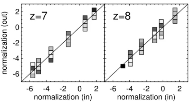
-6 -4 -2 0 2

normalization (in) -6

-4 -2 0 2

normalization (out)

z=7

z=7

-6 -4 -2 0 2

normalization (in)

z=8

z=8

Fig. 8.— Probability distribution function of the recoveredM∗– MUVnormalization as a function of intrinsic normalization atz= 7 andz= 8 in our mock galaxy simulations, when the slope is fixed to the intrinsic slope. When the slope is fixed, the normalization can be recovered at high confidence.

at z= 6. From this simulation, we derive the probabil-ity distribution function of intrinsic slope (slopein) of the

M∗–MUV relation given the observed slope (slopeout),

based on the results from each of the 50 simulations at each input slope. We find, for the given slope ob-served from our real sample, the central 68% range of the intrinsic slope to be −0.57 < slopein < −0.63, −0.42< slopein<−0.53, and−0.42<slopein <−0.64

atz= 4, 5, and 6, respectively. This is comparable with the 1σ confidence level of the observed slope, indicating that our M∗–MUV relations and their uncertainties at

z = 4–6 measured from our real sample are relatively reliable, when we use this optimized method.

It is encouraging that we find no bias atz= 7–8, but the broad PDF of the recovered slope for a given input slope atz= 7–8 indicates that it is hard to constrain the intrinsic slope with the currently available data. There-fore, we perform another test to see if our current data can constrain the normalization of the intrinsicM∗–MUV

relation when we apply an additional prior of a known intrinsic slope. Figure 8 shows the PDF of the recovered normalization as a function of intrinsic normalization at

z = 7–8 when the slope is fixed to the intrinsic slope, illustrating that the normalization can be recovered ac-curately within±0.5.

The best-fit relation for our real sample in Section 4.4 is derived with the optimized method of combining in-dividual bright galaxies with stacks of fainter galaxies. When we need to use the fullM∗–MUVdistribution or a

scatter for our GSMF derivation, we use those inferred atMUV< Mthresh1(z).

4.4. M∗–MUV Relation

Using our optimized method vetted in Section 4.3, we derive the best-fit linear log10(M∗/M)–MUVrelation at

each redshift. Specifically, we use the median mass of in-dividual galaxies for bins with MUV < Mthresh1(z) and

the median mass of median flux-stacked SEDs for bins withMUV< Mthresh2(z). Our best-fit mass-to-light

leav-TABLE 1

Best-fit Fiduciallog₁₀(M∗)–MUVrelation z normalization slope logM∗(MUV=−21)

(M) (M)

4 −1.70±0.65 −0.54±0.03 9.70±0.02 5 −0.90±0.74 −0.50±0.04 9.59±0.03 6 −1.04±0.57 −0.50±0.03 9.53±0.02 7 −1.20±0.16 −0.50± — 9.36±0.16 (−4.23±2.12) (−0.65±0.10) (9.45±0.07) 8 −1.56±0.32 −0.50± — 9.00±0.32

(−5.47±6.19) (−0.69±0.31) (9.00±0.31) Note. — Atz∼7–8, numbers in parentheses are the best-fit parameters when we do not fix the slope to the best-fit slope at z∼6. The quoted errors represent the 1σuncertainties. The normalization is defined as the logarithmic stellar mass at MUV= 0 (logM_∗(M_{UV =0)}).

ing the normalization as a free parameter.16 _{Our mock}

galaxy simulation in Section 4.3 indicates that our cur-rent data allow us an accurate recovery of the intrinsic normalization atz= 7–8 with a prior of a known input slope (Figure 8). We find a (very) weak evolution in the normalization between z = 4 and z = 7 (a decreasing normalization with increasing redshift). The normaliza-tion evolves from log(M∗/M)(MUV=−21)=9.70 (atz=4)

to 9.36 (atz =7) at only 2σ significance. Interestingly, the normalization appears to decrease more rapidly from

z= 7 toz= 8 than at lower redshifts, although the small sample atz= 8 prevents drawing any firm conclusions. We discuss this further in Section 6.

Although theM∗–MUVdistribution of our flux-limited

sample has non-zero scatter, the derivedM∗–MUV

rela-tion is not subject to Malmquist bias (i.e., missing faint galaxies at a given stellar mass) as we estimate theM∗–

MUV relation in bins of luminosity and not stellar mass.

Therefore, the derived relation should be robust against the Malmquist bias, which could artificially result in a steeper slope than the intrinsic one by losing the faint envelope of galaxy distribution for a given stellar mass.17

There are discrepancies of 0.3–0.7 dex between differ-ent studies in the measured median mass at a given UV magnitude even at z ∼ 4, which are larger at fainter UV bins (Gonz´alez et al. 2011; Lee et al. 2012; Stark et al. 2013; Duncan et al. 2014; Salmon et al. 2015). This may reflect a number of systematic uncertainties associ-ated with sample selection and stellar mass estimation. As these uncertainties make a direct comparison between different studies difficult, it highlights the importance of a comprehensive and independent analysis to verify sys-tematics.

Overall, we found the best-fit slope shallower than that of Gonz´alez et al. (2011) but similar to those of Stark et al. (2013) and Duncan et al. (2014) with an excep-tion atz= 4. First, the slope of our best-fit relation of −0.54(±0.03) atz= 4 is significantly shallower than that of Gonz´alez et al. of−0.68, which is based on an order of

16_{Albeit slightly shallower (−(0.44–0.48)), the slope predicted} from the SAMs of Somerville et al. (in prep) is almost constant over the redshift interval as well.

17_{As discussed in Section 4.1, objects with high mass and low} UV flux that we may be missing are believed to be the subdominant population for all UV luminosity bins, and thus would not change the derived relation (see also Salmon et al. 2015 for a similar argu-ment based on the tight scatter of the star-forming main-sequence).

magnitude smaller sample. As the relation of Gonz´alez et al. is derived with no nebular correction, it is not sur-prising that their stellar masses for UV-bright galaxies are higher than ours. However, their stellar masses for galaxies in faint UV bins are lower than ours by∼0.2 dex at MUV ∼ −18, resulting in a steeper slope than ours.

Meanwhile, the M∗–MUV relation of Stark et al. (2013)

shows a good agreement with ours at all redshifts with only a slightly shallower slope than ours. Duncan et al. (2014) in general find higher stellar masses for galaxies that we do in faint UV bins, resulting in a higher normal-ization and a shallower slope than ours, with the biggest difference in normalization (∆ log(M∗/M)MUV=−21 =

0.25) and slope (∆ = 0.09; 2.5σ significance) being ob-served at z= 4 (see Section 5.3 for more discussion).

5. THE GALAXY STELLAR MASS FUNCTION 5.1. Derivation of the GSMFs

We now convolve ourM∗–MUV distribution with the

observed rest-frame UV luminosity function to derive GSMFs. The luminosity functions we utilize in this study are from Finkelstein et al. (2015), which included the full CANDELS GOODS fields, the HUDF and two par-allel fields, and the Abell 2744 and MACS J0416.1-2403 parallel fields from the Hubble Frontier Fields dataset. These luminosity functions are already corrected for in-completeness and selection effects using the detection probability kernels derived from fake source simulations, as discussed by Finkelstein et al. (2015).

Figure 9 presents GSMFs constructed using four dif-ferent methods:

1. “Raw Bootstrapped GSMF”:

We constructed the “observed” GSMF by combining the UV luminosity function with the observedM∗–MUV

distribution. We first drew 105 _{galaxies from the}

best-fit Schechter function of the UV luminosity function in the range of −30 < MUV < −13. Then, we assigned

stellar mass for each galaxy to be the stellar mass of the randomly chosen galaxy with similar rest-frame UV absolute magnitude from the observed M∗–MUV

distri-bution. This method accounts for outliers, which may be a non-negligible fraction of galaxies atz= 4.

The non-negligible spread in stellar mass at a fixed rest-frame UV absolute magnitude observed in Figure 5 can result in GSMFs with an underestimated low-mass-end slope if we donotaccount for the “unobserved” pop-ulation of galaxies below the detection threshold of the survey. This is because galaxies at a given UV luminos-ity have a range of mass-to-light ratios, thus galaxies be-low the detection limit can still have stellar masses high enough to contribute to the number density in the stellar mass bins of our interest (affecting the last few points in the GSMFs depending on the amount of spread). There-fore, we need to correct for the incompleteness by assum-ing aM_∗–MUV distribution in UV luminosity bins below

the current sensitivity limit. We use three different in-completeness correction schemes.

2. “Incompleteness-corrected Bootstrapped GSMF”: A reasonable assumption on theM∗–MUVdistribution

10-5 10-4

10-3 10-2

10-1

φ

[# dex

-1 Mpc -3 ]

Scaled Halo MF

Ilbert+13

Muzzin+13

Stark+09

Lee+12

Gonzalez+11

Duncan+14

Grazian+15

Bootstrapped GSMF Const-scatter GSMF Asymmetric-scatter GSMF

logM* _{= 10.44}+0.19

-0.18

α = -1.53+0.07

-0.06

logφ* = -3.52+0.21

-0.21

z

∼

4

Stark+09

Lee+12

Gonzalez+11

Duncan+14

Grazian+15

logM* _{= 10.47}+0.20

-0.20

α = -1.67+0.08

-0.07

logφ* = -3.87+0.25

-0.28

z

∼

5

10-5

10-4 10-3

10-2

10-1

φ

[# dex

-1 Mpc -3 ]

Stark+09

Gonzalez+11

Duncan+14

Grazian+15

logM* _{= 10.30}+0.14

-0.15

α = -1.93+0.09

-0.09

logφ* _{= -4.52}+0.26

-0.27

z

∼

6

8 9 10 11

log10(M*/MO •)

Gonzalez+11

Duncan+14

Grazian+15

logM* _{= 10.42}+0.19

-0.18

α = -2.05+0.17

-0.17

logφ* _{= -5.16}+0.43

-0.50

z

∼

7

7 8 9 10 11

log10(M*/MO •)

10-6

10-5

10-4

10-3 10-2

10-1

φ

[# dex

-1 Mpc -3 ]

logM* _{= 10.41}+0.19

-0.19

α = -2.45+0.34

-0.29

logφ* = -6.50+0.68

-0.77

z

∼

8

observed distribution of individual galaxies in bright UV bins above a threshold represents the intrinsic distribu-tion and can be extended to fainter bins. In Secdistribu-tion 4.3, we found the redshift-dependent thresholdMthresh1(z) at

each redshift above which the intrinsic distribution can be recovered well without any noticeable bias or increase in scatter. We extend the observed M∗–MUV

distribu-tion at MUV < Mthresh1(z) to fainter UV luminosities

down toMUV =−13, keeping the distribution centered

around the best-fit M∗–MUV relation. The rest of the

procedures are the same as those for the “raw boot-strapped GSMF”.

3. “Constant-scatter GSMF”:

Instead of using individual points in theM∗–MUV

dis-tribution, we assumed an idealized log-normal distribu-tion around the best-fit M∗–MUV relation with a

con-stant scatter, inferred from bright UV luminosity bins that have a statistical number of galaxies and high com-pleteness. We used the mean scatter estimated from the two faintest bins atMUV< Mthresh1(z) with more than

10 galaxies, which is∼(0.4–0.5) dex. The UV luminosity function was then convolved with this log-normal distri-bution to derive the “constant-scatter GSMF”.

4. “Asymmetric-scatter GSMF”:

The three approaches above are basically the same as those used by Gonz´alez et al. (2011). However, the mass distribution of our sample in a given rest-frame UV abso-lute magnitude bin is not symmetric with respect to the best-fit relation. Rather, the lower side of the best-fit re-lation has in general a smaller scatter. As already noted in Section 4.1, the lack of galaxies with high UV luminos-ity and low mass contributes in part to the asymmetric scatter, and the results in Section 4.3 in addition indi-cate that it could be an intrinsic property and not just an observational bias. Therefore, we assume a log-normal distribution with an asymmetric scatter with respect to the best-fit M∗–MUV relation (a different sigma above

and below the mean) inferred from the two faintest bins at MUV < Mthresh1(z) and extend it to fainter UV

lu-minosity bins.18 _{The resultant GSMF constructed via}

this method is referred to as the “asymmetric-scatter GSMF”, and we consider this our fiducial GSMF.

Figure 9 shows the GSMFs at z = 4–8 derived from the four methods described above. The incompleteness-corrected, constant scatter, and asymmetric scatter methods yield consistent results, and their Schechter fits (see Section 5.2) are nearly indistinguishable within the uncertainties.

5.2. Schechter Fit and Uncertainties

Before we parameterize our GSMF with a Schechter function, we first need to derive the uncertainties for our GSMF data points. Randomly perturbing points of the GSMFs is not a proper way to estimate the uncertainties of the GSMFs because they are correlated. Thus, we de-rive the 68% confidence interval of our fiducial GSMFs as

18_{Forz= 7 andz= 8 where the scatter is not robustly measured} due to the small sample size, we assume theM∗–MUVdistribution follows that atz= 6.

follows. First, we randomly drew 1,000 samples from an MCMC chain of the UV luminosity function Schechter parameters derived by Finkelstein et al. (2015) within the 3-dimensional 1σ contour of (L∗, αL, φ∗L). Then, for

each luminosity function generated from the Schechter parameters, we assigned aM∗–MUVrelation with (slope,

normalization) values randomly chosen within the 2-dimensional 1σcontour of the best-fit parameters of the

M∗–MUVrelation.19 The newM∗–MUVdistribution was

then combined with the new luminosity function to gen-erate a GSMF in the same way that our GSMF was con-structed. This generates 1,000 GSMFs of which the min-imum and maxmin-imum represent the 1σ upper and lower limits of the GSMFs, respectively.

We parameterize our GSMFs with a Schechter (1976) function,

φ(M∗)dM∗= (φ∗/M∗)×(M∗/M∗)αexp[−(M∗/M∗)]dM∗ (1) which is characterized by a power law with a low-mass-end slope of α, an exponential cut-off at stellar masses larger than a characteristic mass, M∗_{, and a} normal-ization φ∗_{. The best-fit, uncertainties, and posterior} distributions of the Schechter parameters for our fidu-cial asymmetric-scatter GSMFs were derived by run-ning a Markov Chain Monte Carlo (MCMC) algorithm that samples the 3-dimensional parameter space of the Schechter parameters. To ensure full coverage of the pa-rameter space and assess convergence, we ran 5 parallel chains comprised of 105 _{steps each. The starting}

posi-tion of the chain was determined by a coarse grid search that minimized the χ2 _{statistic between the model and}

the data. The first 10% of steps were disregarded in the burn-in phase before running each chain to reduce the de-pendance of the posterior distribution on the initial po-sition. The proposal distribution of each parameter was assigned as a normal (log-normal) distribution forα(M∗ andφ∗) with the width tuned to generate an acceptance rate of ∼ 23–30%. As a prior, we limited the sampling parameter space to beα >−10, 8<log(M∗/M)<13, and log(φ∗_/Mpc−3_{) > −8. For 6 ≤ z ≤ 8 where the}

constraints onM∗ are weak (see the large error bars on the open grey circles in Figure 10), we took a log-normal prior on M∗ with mean log(M∗/M) =10.45 and stan-dard deviation of 0.2 dex, following the posterior distri-bution ofM∗_{atz= 4. Comparing the likelihood of the} current step, which is defined as L ∝ e−χ2_/2

, with the proposed set of parameters determines if the proposal is accepted. We employ the Metropolis-Hastings algorithm for the acceptance criteria. After running all chains, con-vergence was assessed by examining trace plots of param-eters as well as using the Rubin-Gelman ˆR diagnostic (Gelman & Rubin 1992) for each marginalized posterior distribution. The diagnostic value ˆR∼ 1 suggests con-vergence, and we confirmed that for all redshifts and pa-rameters, the diagnostic has a value 1.00<R <ˆ 1.02.

From the resulting joint posterior distribution, we ex-tracted the marginal posterior distribution of each pa-rameters. The median and the central 68% of the marginal posterior distributions provide our fiducial

19_{Forz=7–8 where we fix the slope of theM}