GAEP.pdf

The GAEP algorithm for the fast computation of

the distribution of a function of dependent

random variables

Philipp Arbenz

Paul Embrechts

Giovanni Puccetti

September 1, 2010

Abstract

We introduce a new algorithm for numerically computing the distribution of an increasing function ofddependent, non-negative random variables with given joint distribution. We prove convergence of the algorithm and give con-vergence rates under regularity conditions.

Key words:Distribution functions; dependent random variables.

AMS Subject Classfication:62E17; 65C20; 65C50.

1 Introduction

In this paper, we introduce the GAEP algorithm in order to computeP[ϕ(X)_≤s], whereXis a random vector in (0,_∞)d andϕis a continuous function, strictly in-creasing in each coordinate. The algorithm is based on the decomposition of the set {x_∈(0,_∞)d:ϕ(x)_≤s} into a countable family of disjoint hypercubes. The cor-responding probabilityP[ϕ(X)≤s] is then approximated by the measure over these hypercubes.

The GAEP (Generalized AEP) algorithm is similar in spirit to the AEP algorithm introduced by the same authors in Arbenz et al. (2010) for the caseϕ(x)=Pd

k=1xk.

As the two algorithms are based on different geometrical decompositions, GAEP is not a proper extension of AEP.

The paper is organized as follows. After some preliminaries in Section 2, we il-lustrate GAEP in dimension two (d ₌2) in Section 3. Section 4 extends GAEP to arbitrary dimensions, its convergence being discussed in Section 5, 6 and 7. In Sec-tion 8, we test GAEP on some examples, and, in SecSec-tion 9, we compare and contrast it to its main competitors. Section 10 illustrates the differences between GAEP and AEP, while, in Section 11, we provide a method to improve convergence rates in di-mension three. Section 12 concludes the paper.

∗_{[email protected], Department of Mathematics, ETH Zurich, 8092 Zurich, Switzerland}

†_{[email protected], Department of Mathematics, ETH Zurich, 8092 Zurich, Switzerland} ‡_{[email protected], Department of Mathematics for Decisions, University of Firenze,}

2 Notation and preliminaries

Fixd∈N,d≥2, and defineN=2d. We setR₊=[0,+∞) andR₋=(−∞, 0]. Through-out the paper, (row) vectors are denoted in boldface, for example,ek∈Rdis thekth standard unit vector, fork∈D={1, . . . ,d}. We writei1, . . . ,iN for all the 2d vectors in {0, 1}d, that is,i1=0=(0, . . . , 0),ik+1=ek,k∈D, and so on,iN=1=(1, . . . , 1). By #i=Pd

k=1ik, we denote the number of 1’s in the vectori, for example, #i1=0, #iN=

d. We define the componentwise product between two vectorsx=(x1, . . . ,xd),y= (y1, . . . ,yd)∈Rdas

x◦y=(x1y1, . . . ,xdyd)∈Rd.

For instance,x◦ek=xkek=(0, . . . , 0,xk, 0, . . . , 0). Let≥denote the componentwise order between vectors, that is,x_≥yif and only ifxk≥ykfor allk∈D. The orders≤,

<and_>are defined analogously.

On some probability space (Ω,A,P), assume that the random vectorX₌(X1, . . . ,Xd) has joint distributionH. Throughout the paper, we assume the marginal compo-nentsXkto be non-negative, i.e. P[Xk≤0]=0 for allk∈D. The extension to ran-dom vectors bounded from below is straightforward and will be illustrated in the following. The joint distributionHinduces the probability measureVHonRdvia

VH

h ©

y_∈Rd:y_≤xªi

=H(x) , for allx_∈Rd.

Forb_∈Rdandh_∈Rd_−∪Rd₊, we define the hypercubeQ(b,h)_⊂Rdas

Q(b,h)= (©

x∈Rd:b<x≤b+hª

, ifh∈Rd+, ©

x_∈Rd:b₊h_<x_≤bª

, ifh_∈Rd₋. (1)

Forh_∈Rd₊, theVH-measure ofQ(b,h) can be calculated easily as

VH[Q(b,h)]=P[X∈Q(b,h)]= N

X

j=1

(₋1)d+#ij_H¡ b₊h_◦ij

¢

. (2)

The caseh∈Rd−is analogous. As a special case of (2) ford=2, the probability

mea-sure of a rectangle_Q(b,h)₌(b1,b1+h1]×(b2,b2+h2] can be written as

VH[Q(b,h)]=H(b1,b2)−H(b1+h1,b2)−H(b1,b2+h2)+H(b1+h1,b2+h2).

LetN be the set of continuous functionsϕ:Rd_→R, which are strictly increasing in each coordinate, and such that

lim

t→+∞ϕ(b+tek)= +∞, and t→−∞lim ϕ(b+tek)= −∞, for all b∈R

d _andk

∈D.

Forb∈Rdandp∈Rd−∪Rd+we also define thequasisimplexS(b,p) as

S(b,p)= (©

x_∈Rd:b_<x_≤b₊p,ϕ(x)_≤sª

, ifp_∈Rd₊,

©

x∈Rd:b+p<x≤b,ϕ(x)>sª

, ifp∈Rd−.

(3)

Note that, if one or more of the components ofhandpare equal to zero, thenQ(b,h) andS(b,p) are empty.

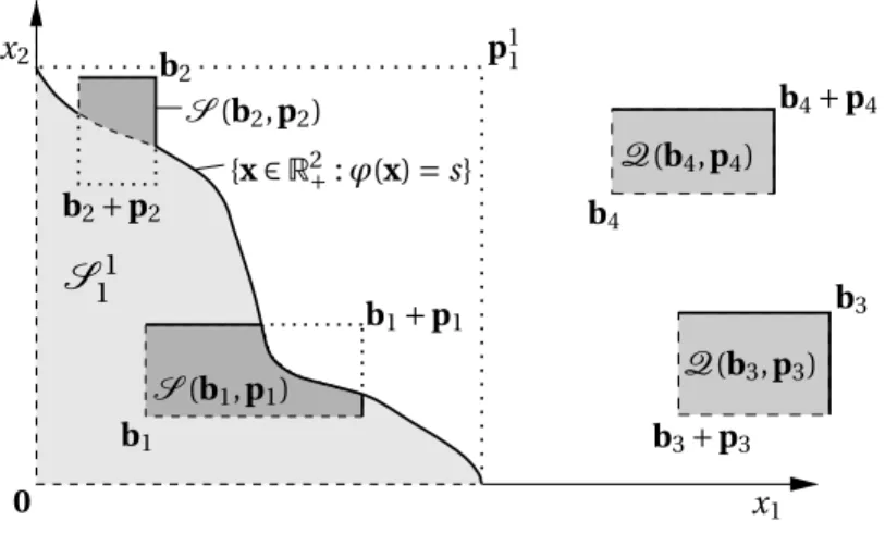
Sinceϕ∈N, there exists a unique vectorp1₁∈Rd+such that

ϕ(p1₁◦ek)=s, for allk∈D. (4)

Figure 1 illustrates (3) and (1) as well as (4) ford=2. DefiningS₁1=S(0,p1₁) and recalling thatXis non-negative, (4) implies that

P£

ϕ(X)≤s¤

=VH£S11

¤

.

b₁

S(b2,p2)

b2

b1+p1

S

1

x2

b2+p2

0

{x∈R2₊:ϕ(x)=s}

x1

b4+p4

b3

b3+p3

p1₁

Q(b4,p4)

Q(b3,p3)

S(b1,p1)

b4

Figure 1: Three quasisimplexesS₁1=S(0,p1₁),S(b1,p1),S(b2,p2)⊂R2and two

hypercubesQ(b3,p3),Q(b4,p4)⊂R2withp11,p1,p4∈R2+andp2,p3∈R2−. Thick and

dashed lines indicate closed and, respectively, open boundaries of the sets.

3 Description of the GAEP algorithm in dimension

d

₌

2

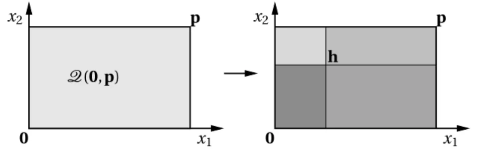
Leth∈R2+such thath≤p11. For ease of notation, we writep=p11throughout this

section. As illustrated in Figure 2, the rectangleQ(0,p)⊂R2can be split into four disjoint rectangles along the components ofh, as

Q(0,p)=Q(0,h)∪Q¡

(h1, 0), (p1−h1,h2)

¢ ∪Q¡

(0,h2), (h1,p2−h2)

¢ ∪Q¡

h,p−h¢

. (5)

A similar decomposition holds for the quasisimplexS(0,p), for which we have

S(0,p)_=S(0,h)_∪S((h1, 0), (p1−h1,h2))∪S((0,h2), (h1,p2−h2))∪S(h,p−h).

(6)

Note that S(0,h)=Q(0,h) \S(h,−h). By setting S₁1=S(0,p), Q1₁=Q(0,h),

p

x

0

x

p

x

0

x

Q

(

0

,

p

)

h

Figure 2: An illustration of (5), where the rectangleQ(0,p)⊂R2is decomposed into four disjoint rectangles.

S1

2 =S(h,−h),S22=S((h1, 0), (p1−h1,h2)),S23=S((0,h2), (h1,p2−h2)) andS24=

S(h,p−h), we can reformulate (6) as

S1 1 =

¡

Q1 1\S21

¢

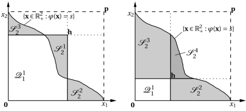
∪S22∪S23∪S24, (7)

as illustrated in Figure 3. Note that eitherS₂1= ;(ifϕ(h)>s) orS₂4= ;(ifϕ(h)≤s).

Since theS₂t’s are disjoint andS₂1⊂Q11, (7) translates into the decomposition

VH£S11

¤

=VH£Q11

¤

−VH£S21

¤

+VH£S22

¤

+VH£S23

¤

+VH£S24

¤

. (8)

As a first approximation ofVH[S₁1] we take the valueP1=VH[Q₁1]. Thus, the differ-ence betweenP1andVH[S₁1] is given by

VH£S11

¤ −P1=

4

X

t=1

τt

2VH£S2t

¤

,

whereτ₂t_∈{₋1, 1} indicates whether the measureVH[S2t] has to be added (τ22=τ32=

τ4

2=1) or subtracted (τ12= −1).

Q

Q

S

S

S

h

0 0

h

x2 x2

x1

x1

S

S

S

{x∈R2+:ϕ(x)=s}

{x∈R2₊:ϕ(x)=s} p p

Figure 3: An illustration of the decomposition (7) for two different choices ofh∈

Rd

−∪Rd+. In the left picture, we haveϕ(h)>sandS24= ;, while, in the right picture,

we haveϕ(h)_<sandS₂1_{= ;}.

The measure of the four squares so obtained is to be added or subtracted toP1in

order to define a second estimateP2ofVH[S₁1], so that the difference betweenP2

andVH[S₁1] will be given by the measure of the remaining sixteen quasisimplexes. The latter are then decomposed again in the following step of the algorithm. By iterating this procedure, we obtain a sequencePn of estimates which we will prove to converge toVH[S₁1] under the regularity conditions given in Section 5. In the general case, at each iteration of the algorithm, we restrict to quasisimplexes which turn out to be nonempty.

4 Description of the GAEP algorithm in arbitrary

dimen-sions

In this section, we state the two main results of the paper. First, we will extend the measure decomposition (8) to arbitrary dimensions, by showing that the measure of an arbitrary quasisimplex can be decomposed into the measures of a hypercube andN₌2d smaller quasisimplexes. Then, we define a sequencePn which will be proved to converge toVH[S11].

Forp∈Rd−∪Rd+, fixh∈H(p), where

H(p)₌

(©

x∈Rd:0≤x≤pª

, ifp∈Rd+, ©

x_∈Rd:p_≤x_≤0ª

, ifp_∈Rd₋.

Lemma 1. For an arbitrary hypercubeQ(b,p)⊂Rd, we have

Q(b,p)₌ N

[

j=1

Q¡

b₊ij◦h,ij◦p+(1−2ij)◦h

¢

, (9)

with the hypercubes on the right-hand side of(9)being disjoint.

Proof. Forj=1, . . . ,N, let the setsCjbe defined as

Cj={x∈Rd:xk≤bk+hkfor allkwith (ij)k=0,xk>bk+hkfor allkwith (ij)k=1}.

SinceSN

j=1ij ={0, 1}

d_{, we have that the family {C}

j,j=1, . . . ,N} is a partition ofRd, that is,Ci∩Cj= ;andSN_j=1Cj=Rd. Hence, we can write

Q(b,p)=

N

[

j=1

¡

Q(b,p)∩Cj¢.

Ifp∈Rd+(the casep∈R−d is analogous), note that for allj =1, . . . ,N andk∈D, we

have

¡

b₊ij◦h

¢

k=

(

bk, if (ij)k=0, bk+hk, if (ij)k=1,

(10)

¡

ij◦p+(1−2ij)◦h

¢

k=

(

hk, if (ij)k=0, pk−hk, if (ij)k=1.

(11)

Thus, the result follows by observing that

Q(b,p)∩Cj=

n

x∈Rd:bk<xk≤bk+hkfor allkwith (ij)k=0,

bk+hk<xk≤pkfor allkwith (ij)k=1

o

=Q¡

b+ij◦h,ij◦p+(1−2ij)◦h¢.

The set decomposition (9) translates into the measure decomposition given by the following theorem.

Theorem 2. Letv1, . . . ,vN∈{0, 1}dbe defined asv1=1andvk=ikfor k=2, . . . ,N . Let

b∈Rd,p∈Rd−∪Rd+andh∈H(p). Then

VH

£

S(b,p)¤

=VH[Q(b,h)]+ N

X

j=1

mjVH

£

S¡

b₊vj◦h,ij◦p+(1−2vj)◦h

¢¤

, (12)

Proof. First assume thatϕ(b)≤sandp∈Rd₊. Defining the setΛ={x∈Rd:ϕ(x)≤s}, and using (9), we can write

Λ∩Q(b,p)=S(b,p)=[Nj=1

©

Λ∩Q¡

b+ij◦h,ij◦p+(1−2ij)◦h¢ª

=[Nj=1S

¡

b₊ij◦h,ij◦p+(1−2ij)◦h

¢

. (13)

Since the hypercubes on the right-hand side of (9) are disjoint, the quasisimplexes on the right-hand side of (13) are disjoint, too. Thus, from (13), we get

VH£S(b,p)¤= N

X

j=1

VH£S¡b+ij◦h,ij◦p+(1−2ij)◦h¢¤. (14)

Sincei1=0, we have

VH[S(b+i1◦h,i1◦p+(1−2i1)◦h)]=VH[S(b,h)], and we can write (14) as

VH£S(b,p)¤=VH[S(b,h)]+ N

X

j=2

VH£S¡b+ij◦h,ij◦p+(1−2ij)◦h¢¤. (15)

Noting thatS(b,h)=Λ∩Q(b,h), and using the fact thatQ(b,h)=Q(b+h,−h),we obtain

VH[S(b,h)]=VH[Λ∩Q(b,h)]=VH[Q(b,h)]−VH[Q(b+h,−h)∩ΛC]

=VH[Q(b,h)]−VH[S(b+1◦h,0◦p+(1−2·1)◦h)]. (16)

Substituting (16) in (15), and recalling the definition of thevj’s, we finally get (12). The caseϕ(b)>s,p∈Rd−is analogous. The casesϕ(b)≤s,p∈Rd−, andϕ(b)>s, p_∈Rd₊, are trivial, since they implyVH[S(b,p)]=0 andVH[Q(b,h)]=VH[S(b+

h,₋h)].

Note that Theorem 2 holds for all measurable functionsϕ:Rd_→R.

The idea behind the GAEP algorithm is to apply the decomposition (12) recur-sively to the nonempty quasisimplexes on the right side, starting withS₁1₌S(0,p1₁),

p1₁being the unique vector satisfying (4). Note that, by changing the conditions (4) and the vectorb1₁, the algorithm can be applied to the case in which the random vec-torXalso takes negative values but it is still bounded from below, as, for example,

P[X≥b1₁]=1.

At the beginning of thenth iteration (n∈N), the algorithm receives, as input, a family

St

n =S(btn,ptn),t∈In⊂{1, . . . ,Nn−1}

of nonempty quasisimplexes. As already remarked, forn₌1 we haveI1={1} and

S1

1 =S(0,p11). Given a sequence of splitting pointsh

t

qua-sisimplexS_ntis then decomposed into one hypercube andNquasisimplexes via (12):

VH£S(btn,ptn)

¤

=VH£Q(btn,htn)

¤ +

N

X

j=1

mjVH£S¡bnt+vj◦htn,ij◦pnt+(1−2vj)◦htn

¢¤

=VH£Q(btn,htn)

¤ +

N

X

j=1

mjVH

h

S³b_nN t₊−₁N+j,p_nN t₊₁−N+j´i,t∈In,

(17)

where the sequencesb_nt andpt_nare defined by their initial valuesb1₁=0andp1₁, and by

b_nN t₊−₁N+j₌b_nt₊vj◦hnt, (18)

pN t_n+−₁N+j₌ij◦pnt+(1−2vj)◦htn, (19) for allj₌1, . . . ,N andt_∈In. Recall from Theorem 2 thatm1= −1 andmj =1 for j₌2, . . . ,N. At this point, the family of nonempty quasisimplexes obtained on the right-hand side of (17),

S(bt_n+1,pt_n+1),t_∈In+1, with In+1={t∈{1, . . . ,Nn} :S(bnt+1,ptn+1)6= ;},

is passed to the (n+1)th iteration of the algorithm.

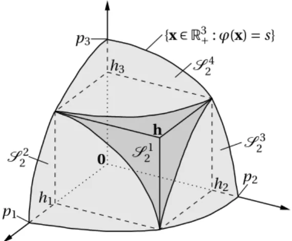
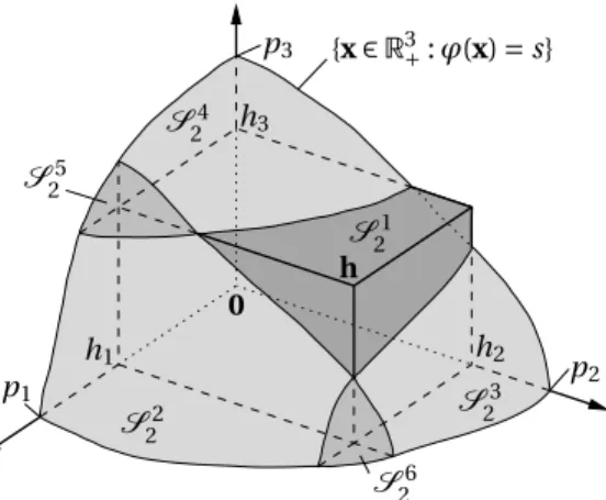
As an example, we illustrate the first iteration of the algorithm in the cased=3, where we denotep1₁=pwith0≤h≤p. For the simplexS₁1=S(0,p), the measure decomposition (12) gives

VH[S(0,p)]=VH[Q(0,h)]−VH[S(h,−h)]+VH[S((h1, 0, 0), (p1−h1,h2,h3))]

+VH[S((0,h2, 0), (h1,p2−h2,h3))]+VH[S((0, 0,h3), (h1,h2,p3−h3))]

+VH[S((h1,h2, 0), (p1−h1,p2−h2,h3))]+VH[S((h1, 0,h3), (p1−h1,h2,p3−h3))]

+VH[S((0,h1,h2), (h1,p2−h2,p3−h3))]+VH[S(h,p−h)].

In Figure 4, we illustrate the case in whichϕ(p◦ek)=s,k∈D(see conditions (4)),

ϕ(h1,h2, 0)≤s,ϕ(h1, 0,h3)≤sandϕ(0,h2,h3)>s, leading toS₂7=S₂8= ;.

There-fore, we haveI1={1} andI2={1, 2, 3, 4, 5, 6}. Note also that, in the two-dimensional

cases described in Figure 3, we hadI2={1, 2, 3} (left) andI2={2, 3, 4} (right).

In general, the set of indexesIn+1, which identifies the quasisimplexesSnt+16= ;,

depends on the vectorsht_n,t_∈In and on the functionϕ, at each iteration of the algorithm. Nevertheless, for a fixedn, the quasisimplexesS_nt₊₁,t_∈In+1, are always

disjoint (this follows from the proof of Theorem 2).

Now, define the familyQ_nt =Q(b_nt,ht_n),t∈In, and the sequencePnas the sum of theVH-measures of all theQnt’s multiplied by the correspondingτtn, as

Pn=Pn−1+

X

t∈In τt

nVH

£

Qt n

¤ =

n

X

i=1

X

t∈Ii τt

iVH

£

Qt i

¤

,n_∈N, (20)

whereP0=0 and the sequenceτnt is defined by its initial valueτ11=1 and by

τN t−N+j

n+1 =τ

t

{x∈R3₊:ϕ(x)=s}

S3 2

S4 2

S1 2

h2

h3

h1

S6 2

S2 2

p3

p2

p1

0

h

S5 2

Figure 4: An illustration of the decomposition (12) ofS(0,p)_⊂R3for some vector

h_∈Rd₊.

The valueτt_n∈{₋1, 1} indicates whether the measure of the quasisimplexS_nthas to be added (τt_n=1) or subtracted (τt_{n= −}1) in order to compute an approximation of VH[S11].

We now show that, at each iteration of the algorithm, the error committed by takingPnas an approximation ofVH

£

S1 1

¤

can be expressed in terms of the measures of the nonempty quasisimplexesS_nt₊₁,t∈In+1passed to the (n+1)th iteration of the

algorithm.

Theorem 3. With the notation introduced above, we have that

VH

£

S1 1

¤ −Pn=

X

t∈In+1

τt n+1VH

£

St n+1

¤

. (22)

Proof. We proceed by induction onn. Recalling thatτ1₁₌1 andP0=0, (22)

corre-sponds, forn=0, to the trivial equalityVH

£

S1 1

¤ =VH

£

S1 1

¤

. Hence, suppose that (22) holds for somen∈N. Substituting (17) in (22), and using (20), yields

VH

£

S1 1

¤ =Pn+

X

t∈In+1

τt n+1VH

£

Qt n+1

¤ + X

t∈In+1

τt n+1

Ã_N X

j=1

mjVH

h

SN t−N+j n+2

i !

=Pn+1+

X

t∈In+1

N

X

j=1

τt

n+1mjVH

h

SnN t+2−N+j

i

.

Recalling (21), we get

VH

£

S1 1

¤

=Pn+1+

X

t∈In+1

N

X

j=1

τN t−N+j n+2 VH

h

SN t−N+j n+2

i

=Pn+1+

X

t∈In+2

τt n+2VH

£

St n+2

¤

,

where the last equality follows from the fact that the simplexesS_nt₊₂,t∉In+2, are

5 Convergence of the algorithm

In this section, we give sufficient conditions for the convergence of the sequence Pn, defined above, to the valueVH

£

S1 1

¤

. First, in Lemma 4, we give a simple set rep-resentation ofPn. Recall that the setIn+1identifies the non empty quasisimplexes

St

n+1,t∈In+1, which are passed to the (n+1)th iteration of the algorithm. We

parti-tion the setIn+1into the families

I+_n+1={t∈In:τnt+1= +1} andI−n+1={t∈In:τtn+1= −1}.

Lemma 4. For any n_∈N,we have that Pn=VH[Bn], where

Bn=

Ã

S1 1

[

t∈I− n+1

St n+1

!

\ [ t∈I+_n+1

St

n+1. (23)

Proof. Using induction, we prove that, for a fixednand allt_∈In, we have

St n⊂

(

S1

1, ifτtn= +1, Q(0,p1₁) \S₁1, ifτt_n= −1.

Then, the result easily follows from (22) and the fact that, for a fixedn, theS_nt₊₁’s are disjoint.

From its definition (3), a quasisimplexS(b,p) lies inS₁1if and only ifp_∈R+

d. It lies instead inQ(0,p1₁) \S₁1if and only ifp∈R−_d. Therefore, we equivalently have to show that, for a fixednand allt∈In,

pt_n∈ (

R+

d, ifτ t n= +1,

R−

d, ifτ t n= −1.

(24)

To this end, assume that (24) is true for a fixedn(forn₌1, it trivially holds) and choose an arbitraryS_nt₊₁,t_∈In+1such thatτnt+1= +1 (the caseτ

t

n+1= −1 is

anal-ogous). By (21), there existt0_∈I

n andj ∈{1, . . . ,N}, withτtn+1=τ

N t0_−N+j

n+1 =τ

t0

nmj. Sinceτ_nt₊₁= +1, either (case I)τ_nt0= −1 andmj = −1 (in this case,j=1) or (case II)

τt0

n =1 andmj= +1 (in this case,j6=1).

Case I:If j₌1, using (19) we obtainp_nN t₊0₁−N+j = −h_nt0. Since it also holds thatτt_n0= −1, using the induction assumption, we obtain thatpt_n∈R−d and finally (recall that

h_nt _∈H(p))p_nN t₊0₁−N+j_{= −}ht_n∈R+

d. Case II:Forj₆₌1, (11) yields

(pN t_n+0₁−N+j)k=

(

(h_nt0)k, if (ij)k=0,

(p_nt0−h_nt0)k, if (ij)k=1.

Since it also holds thatτt_n0 = +1, using the induction assumption, we obtain that

A simple illustration of (23) in dimensiond=2 is given by (7) and by the corre-sponding Figure 3. Now, we use Lemma 4 to obtain bounds onPn.

Theorem 5. Ifϕ∈N then, for all n∈N, we have

P£

ϕ(X)≤ln¤≤Pn≤P£ϕ(X)≤un¤, (25)

where

ln=min

©

s, min t∈I+

n+1

ϕ(bt_n+1)ª

and un=max

©

s, max t∈I−

n+1

ϕ(bt_n+1)ª

.

Proof. Suppose that, for a quasisimplexS_nt₊₁, we haveτt_{n+1= −}1. Then (see (24))

p_nt_+1≤0. Therefore, over the quasisimplexS_nt₊₁, the functionϕ_∈N attains its maximum atb_nt₊₁, i.e.

max x∈St

n+1

ϕ(x)=ϕ(b_nt₊₁).

Using the above result and (23), we can write

Bn⊂S11

[

t∈I− n+1

St n+1⊂

n

x∈Rd+:ϕ(x)≤max ©

s, max t∈I−_n+1ϕ(b

t n+1)

ªo

,

which yields_Bn⊂©

x∈Rd+:ϕ(x)≤un

ª

. Recalling from Lemma 4 thatPn=VH[Bn], the right-hand side of (25) follows. Analogously, ifτt_{n+1= +}1, we have thatpt_n+1≥0

and

inf x∈St n+1

ϕ(x)₌ϕ(b_nt₊₁).

Recalling thatb_nt_+1∉Snt₊₁whenpt_n+1≥0, we obtain that_ϕ(bt_n+1)_<ϕ(x) for allx_∈

St

n+1. Using again (23), it follows that

n

x∈Rd+:ϕ(x)≤min ©

s, min t∈I+

n

ϕ(bt_n+1)ªo ⊂S11\

[

t∈I+ n+1

St

n+1⊂Bn,

which yields©

x_∈Rd₊:_ϕ(x)_≤ln

ª

⊂Bnand, consequently, the left-hand side of (25).

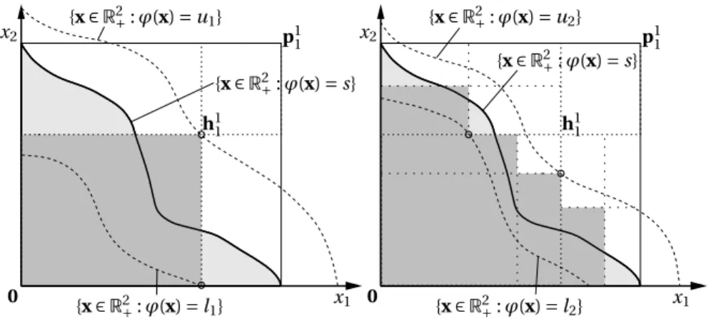
Figure 5 illustrates Theorem 5 for the first two iterations of the algorithm in the cased₌2. Now, we define the sequenceDn,n∈N, as

Dn=max {s−ln,un−s}=max t∈In+1

¯

¯ϕ(bt_n+1)−s ¯

¯. (26)

The following lemma will turn out to be useful in the remainder of the paper.

Lemma 6. Ifϕ_∈N, then, for all n_∈N, we have

¯

¯P_n−V_H[S₁1] ¯

0

x2

h1₁

x1 {x∈R2+:ϕ(x)=l1}

{x∈R2+:ϕ(x)=u1}

x2

h1₁

{x∈R2+:ϕ(x)=l2} {x∈R2+:ϕ(x)=u2}

x1 0

{x∈R2+:ϕ(x)=s} {x∈R2+:ϕ(x)=s}

p1₁ p1₁

Figure 5: An illustration of Theorem 5 ford=2,n=1 (left) andn=2 (right). The dark grey area identifies the setsB1=Q₁1(left) andB2=(Q₁1∪Q₂3∪Q₂3∪Q4₂) \Q₂1

(right). We seth4₂=0, thusQ₂4= ;. The circles indicate whereϕattains either its maximum or its minimum.

Proof. From (25) and (26), we have that

Pn≤P[ϕ(X)≤un]≤P[ϕ(X)≤s+Dn].

SinceDn≥0, we obtain

Pn−VH[S11]≤P[ϕ(X)≤s+Dn]−P[ϕ(X)≤s]

=P[s<ϕ(X)≤s+Dn]≤P[s−Dn<ϕ(X)≤s+Dn].

Analogously, we can write

Pn−VH[S11]≥P[ϕ(X)≤s−Dn]−P[ϕ(X)≤s]

= −P[s₋Dn<ϕ(X)≤s]≥ −P[s−Dn<ϕ(X)≤s+Dn].

Recall the definition ofDnin (26).

Theorem 7. AssumeXis absolutely continuous andlimn→∞Dn=0. Then

lim n→∞Pn=P

£

ϕ(X)_≤s¤

=VH[S11].

Proof. If limn→∞Dn =0, andϕ(X) is continuous, then the theorem follows from Lemma (6). Therefore, it is sufficient to show thatP[ϕ(X)=s]=0, for alls ∈R. Fix somes ∈R, and let Γs ={x∈Rd :ϕ(x)=s}. Sinceϕ∈N, for eachy∈Rd−1 there exists a uniquezy∈Rsuch thatϕ(y1, . . . ,yd−1,zy)=s. It is easy to see that

Note that, in Theorem 7, the assumption of absolutely continuity ofXcannot be dropped. As a counterexample, taked=2 andX=(U, 1−U), whereUis a random variable uniformly distributed on [0, 1]. For the functionϕ(x)=x1+x2, we have that

Xis continuous, whileP[ϕ(X)=1]=1. In this case, and depending on the sequence

h_nt, the sequencePnmay fail to converge.

6 The choice of the h

: the bisection rule

Assuming continuity ofϕ(X), convergence of the GAEP algorithm is guaranteed by Theorem 7 whenever the sequenceDn goes to zero. Of course, the (speed of ) con-vergence of the sequenceDn depends on the choice of the vectors {htn,t∈In}, at each iteration. The aim of this and the following section is to find good criteria for the choice of theht_nsuch thatDnconverges (rapidly) to 0.

Note that, wheneverS_nt₌Q(bt_n,pt_n), in (17) it is convenient to seth_nt ₌pt_n, so that no simplexes are passed on to the following iteration of the algorithm. In fact, using (19), havinght_{n =}pn_t implies thatSN t−N+1

n+1 =S(b

t

n+pnt,−ptn)=Q(btn,ptn) \ St

n = ;. Moreover, for j =2, . . . ,N, (11) implies that at least one component of

pN t_n+−₁N+jis zero, henceS_nN t₊₁−N+j= ;.

As a first choice forht_n, we propose the so-calledbisection rule. Using this choice, convergence of the sequenceDnis guaranteed under some extra assumptions onϕ.

Theorem 8. Assume that_ϕ∈N0_{, the set of all twice differentiable functionsϕ∈N}

for which there exists a constant r_>0such that_∂kϕ(x)>r for all k∈D andx∈Rd. For all n_∈Nand t_∈In, let the sequencehnt be defined as

ht_n= (

pt_n, ifS_nt=Qnt,

1/2pt_n, otherwise. (27)

Then, Dn=O(2−n) ,n→ ∞.

Proof. It is immediate thatht_n ∈H(p_nt), and henceht_n is correctly defined. Since ϕis twice differentiable, it is also Lipschitz continuous onQ(0,p1₁), the closure of Q(0,p1₁). Thus, there exists a constantL_{< ∞}such that¯

¯ϕ(x)−ϕ(y) ¯ ¯<L

¯ ¯ ¯ ¯x−y

¯ ¯ ¯ ¯for

allx,y∈Q(0,p1₁).

Now, consider the nonempty quasisimplexS_nt₊₁,t∈In+1, for which there exist

t0∈Inandj ∈{1, . . . ,N} such thatS_nt₊₁=SN t

0_−N+j

n+1 . For the quasisimplexSt

0

n , we have that (from the definition (3))_Snt0_=S(b_nt0,pt_n0)_⊂Q(bt_n0,p_nt0). As_Snt_{+16= ;}, (27) implies thatQ(bt_n0,p_nt0) \S_nt0_{6= ;}.

It is then possible to findyt_n0∈Snt0 andzt

0

n ∈Qt

0

n \St

0

n , for which we have that eitherϕ(yt_n0)_≤s,ϕ(z_nt0)_>s (whenp_nt0 _≥0) orϕ(yt_n0)_>s,ϕ(z_nt0)_≤s (whenpt_n0 _≤0). In both cases, continuity ofϕguarantees (by the intermediate point theorem) the existence of a vectorxt_n0on the curvec: [0, 1]7→(1−c)yt_n0+czt_n0, withϕ(xt_n0)=s. Clearly,

xt_n0∈Qt 0

n, and by (18) and (10), alsob N t0_−N+j

n+1 ∈Q

t0

¯ ¯ ¯ ¯ ¯ ¯b

N t0_−N+j

n+1 −xt

0

n

¯ ¯ ¯ ¯ ¯ ¯≤

¯ ¯ ¯ ¯ ¯ ¯p

t0 n

¯ ¯ ¯ ¯ ¯

¯. Therefore, for eacht∈In+1, there existst 0_∈I

nsuch that

¯

¯ϕ(bt_n+1)−s ¯ ¯=

¯ ¯ ¯ϕ(b

N t0_−N+j

n+1 )−s

¯ ¯ ¯=

¯ ¯ ¯ϕ(b

N t0_−N+j

n+1 )−ϕ(x

t0

n)

¯ ¯ ¯≤L

¯ ¯ ¯ ¯ ¯ ¯b

N t0_−N+j

n+1 −x

t0

n

¯ ¯ ¯ ¯ ¯ ¯≤L

¯ ¯ ¯ ¯ ¯ ¯p

t0

n

¯ ¯ ¯ ¯ ¯ ¯.

Combining the above result with the definition ofDngiven in (26), it follows that

Dn=max t∈In+1

¯ ¯ϕ(b_nt

+1)−s

¯

¯≤Lmax

t∈In ¯ ¯ ¯ ¯p_nt

¯ ¯ ¯

¯. ₍₂₈₎

Note that (28) holds for a general sequenceh_nt,t_∈In. Using the definition of the

pN t_n+−₁N+j(see (19)) and the bisection rule (27), it follows that

pN t_n+−₁N+j=ij◦ptn+(1−2vj)◦htn=ij◦ptn+(1−2vj)◦1/2pnt

=(ij+1/2(1−2vj))◦pnt =(ij−vj+1/21)◦ptn=

(

1/2pt_nifj₆₌1,

−1/2pt_nifj=1.

Thus, we have

max t∈In+1

¯ ¯ ¯ ¯p_nt₊₁¯

¯ ¯

¯=1/2 max

t∈In ¯ ¯ ¯ ¯p_nt¯

¯ ¯ ¯.

Using (28), we finally obtain that

Dn≤Lmax t∈In

¯ ¯ ¯ ¯pt_n¯

¯ ¯

¯=1/2Lmax

t∈In−1

¯ ¯ ¯ ¯pt_n−1¯

¯ ¯

¯=(1/2)n−1Lmax

t∈I1

¯ ¯ ¯ ¯pt₁¯

¯ ¯

¯=(1/2)n−1L ¯ ¯ ¯ ¯p1₁¯

¯ ¯ ¯,

which implies the theorem. In the proof above, note that, even ift_∈In+1, there does

not necessarily exist a vectorxt_n+1∈Q_nt₊₁such thatϕ(x_nt₊₁)₌s. This case occurs, for example, whenS_nt₊₁₌Q_nt₊₁.

In order to have convergence of the bisection method, we only needϕto be Lipschitz continuous onQ(0,p1₁). However, to keep notation simple, we defined the smaller set of functionsN0, which we will use in the following section.

7 The choice of the h

: the gradient rule

In this section, we present thegradient method, a different way of choosing the se-quenceht_n, which guarantees a better asymptotic convergence rate in the cased=2. Byx∧y, denote the componentwise minimum ofxandy, and, byx∨y, the compo-nentwise maximum. We keep the assumption thatϕ∈N0, see Theorem 8.

First, we use Taylor expansion to find a constant 0≤R< ∞such that

¯

¯ϕ(b+δ)− ¡

ϕ(b)+ ∇ϕ(b)Tδ¢¯

¯≤R||δ||2_∞,

for allx_∈Q(b,p) andx₊δ_∈Q(b,p), where_∇ϕdenotes the gradient ofϕ. Sinceϕ is twice differentiable, the constantRcan be chosen to be the same for everyb_∈

Theorem 9. Assume thatϕ∈N0and fixα∈(1/d, 1). Forsomen∈Nand all t∈In, let the sequenceht_nbe defined as

ht_n=   

 

p_nt, ifS_nt=Q(b_nt,pt_n), (ht∗

n ∧ptn)∨0, ifSnt6=Q(bnt,ptn),ptn∈Rd+,

(h_nt∗∨pt_n)∧0, ifS_nt6=Q(b_nt,pt_n),pt_n∈Rd−,

(29)

where

¡ h_nt∗¢

k=α

s₋ϕ(bt_n) ∂kϕ(btn)

, for all k∈D.

Then, we have that

Dn+1≤

µ

max{1₋α,αd₋1}₊α2R r2Dn

¶

Dn. (30)

Before proving Theorem 9, we need the following result.

Lemma 10. Assume thatϕ∈N0and fix n∈N. Letht_n,t∈Inbe defined by(29). Then, for all t∈In, we have that

max j:SN t−N+j

n+1 6=;

¯ ¯ ¯ϕ(b

N t−N+j n+1 )−s

¯ ¯ ¯≤

µ

max{1₋α,αd₋1}₊α2R r2

¯

¯ϕ(b_nt)−s ¯ ¯ ¶

¯

¯ϕ(bt_n)−s ¯ ¯.

(31)

Proof. In the caseS_nt₌Q(bt_n,p_nt), there is nothing to prove. Suppose, instead, that ϕ(bt_n)_<s,S_nt₆₌Q(bt_n,pt_n) andp_∈Rd₊, the other non-trivial case whereϕ(bt_n)_>sand

p_∈Rd₋being analogous. It follows from (29) that, for allj_∈1, . . . ,N,

ϕ(bN t_n+−₁N+j)₋s₌ϕ(bt_n+vj◦htn)−s

≤ϕ(bt_n+h_nt∗)−s≤ϕ(b_nt)+ ∇ϕ(bt_n)Tht_n∗−s+R¯¯ ¯ ¯ht_n∗

¯ ¯ ¯ ¯

2

∞

=ϕ(bt_n)₊dα(s₋ϕ(bt_n))₋s₊R¯ ¯ ¯ ¯ht_n∗¯

¯ ¯ ¯

2

∞=(αd−1)(s−ϕ(b

t n))+R

¯ ¯ ¯ ¯h_nt∗¯

¯ ¯ ¯

2

∞.

Recalling that∂kϕ(x)>r,k∈D, we also have thatkhtn∗k∞≤α/r

¯

¯ϕ(bt_n)−s ¯ ¯, which

gives

ϕ(bN t_n+−₁N+j)₋s_{≤ |}ϕ(b_nt)₋s_|

µ

(αd₋1)₊α2R r2|ϕ(b

t n)−s|

¶

. (32)

Note that (vj◦htn)k=pkimpliesS_nN t₊₁−N+j= ;. Hence, for alljwithS_nN t₊₁−N+j6=

;, we havevj◦htn=vj◦htn∗. Thus,

ϕ(bN t_n+−₁N+j)₋s₌ϕ(bt_n+vj◦htn∗)−s

≥ϕ(bt_n)+ ∇ϕ(bt_n)T(vj◦htn∗)−s−R

¯ ¯ ¯ ¯vj◦htn∗

¯ ¯ ¯ ¯

2

As #vj≥1, for allj=1, . . . ,N, we finally get

ϕ(bN t_n+−₁N+j)₋s_{≥ −|}ϕ(bt_n)₋s_|

µ

1₋α₊α2R r2|ϕ(b

t n)−s|

¶

. (33)

Combining (32) and (33) yields (31).

Proof of Theorem 9. First of all, note thatht_n∈H(pt_n), henceht_nis correctly defined. Due to Lemma 10, and recalling thatR>0,we have that

Dn+1=max

t∈In+1|ϕ

(bt_n+1)−s_|

=max t∈In

max j:SN t−N+j

n+1 6=;

|ϕ(bN t_n+−₁N+j)−s_|

≤max t∈In

µ

max{1−α,αd−1}+α2R

r2

¯

¯ϕ(bt_n)−s ¯ ¯ ¶

¯

¯ϕ(b_nt)−s ¯ ¯

= µ

max{1−α,αd₋1}+α2R

r2Dn

¶

Dn.

Now, we are ready to prove convergence of the gradient method.

Theorem 11. Assume thatϕ∈N0and fixα∈(1/d, 1). For somenˆ∈Nandξ∈(0, 1), assume that

max{1−α,αd₋1}+α2R

r2Dnˆ=1−ξ<1. (34)

For all n≥n, let the sequenceˆ h_nt be defined as(29). Then, we have thatlimn→∞Dn=0 and indeed

Dn=O

¡

(max{1₋α,αd₋1})n¢

.

Proof. Using (34) and (30) iteratively, we obtain thatDn≤(1−ξ)n−nˆDnˆfor alln≥nˆ.

Hence, limn→∞Dn=0 and

lim n→∞

Dn+1

Dn ≤ lim n→∞

µ

max{1_−α,_αd₋1}_+α2R r2Dn

¶

=max{1_−α,_αd₋1}.

The condition (34), which guarantees the convergence of the gradient method with a twice differentiable functionϕ, can always be achieved by using the bisection method for the first iterations of the algorithm. In fact, if one defines theht_n us-ing (27), the sequenceDn will go to zero (Theorem 8) and will satisfy (34) for some integer ˆnlarge enough. From that ˆnon, one can then use the gradient method with convergence guaranteed.

Finally, observe thatα∗=d2+1minimizes max{1−α,αd−1} with max{1−α∗,α∗d−

1}=dd−+11. Thus, the rate

Dn=O

µµ_d −1 d₊1

¶n¶

, (35)

8 Applications

In this section, we test the GAEP algorithm on some random vectorsX=(X1, . . . ,Xd) and several functionsϕ. For illustrative reasons, we provide the joint distributionH ofXin terms of the marginal distributionsFXi,i=1, . . . ,d, and a copulaC. For the

theory of copulas and the definition of the Gumbel and Clayton copula families, we refer the reader to Nelsen (2006).

In Table 1, we consider the two-dimensional case (d=2) with Pareto marginals, that is,

FXi(x)=P[Xi≤x]=1−(1+x)

−θi_{,x≥0,i=1, 2,}

with tail parametersθ1=1 andθ2=2. We couple these Pareto marginals via a

Gum-bel copulaC_γGuwith a parameterγ=1.5. For this example, we compute the approxi-mationPn(see (20)) using both the bisection and the gradient method, for different values of the thresholdssand different numbers of iterationsn of the algorithm. Here, we setϕ(x1,x2)=(1+x1)2/3(1+x2)1/3−1. For the gradient method, we

pro-vide the differencesPn−P16and their average computation times, for all iterations

nand thresholds. This has been done to show the speed of convergence of GAEP. The choice ofn₌16 represents the maximum number of GAEP iterations allowed by the memory (4 GB RAM) of our laptop under the gradient method. Within the same table, we give the differencesPn−P18, but using the bisection method. Again,

n₌18 is the maximum number of GAEP iterations under the bisection method. Note that these numbers are different because the number of quasisimplexes pro-duced at each iteration of GAEP and, consequently, the memory used by the algo-rithm, depend on the method chosen. In Table 1, we also compute the ratio

Rn= Dn

s−ϕ(0). (36)

Since, from Lemma 6, we have

¯ ¯P_n−V_H

£

S1 1

¤¯ ¯≤P

·

1₋Rn<ϕ

(X)₋ϕ(0)

s_−ϕ(0) ≤1+Rn

¸

,

the sequenceRn provides a relative measure of convergence of the algorithm. In-deed, the convergence ofRn to 0 implies that the algorithm converges to a certain value. Note that, since analytical values forVH[S₁1] are not available for this ex-ample, nothing can be said about the correctness of the limit. However, for a two-dimensional portfolio, we see that the estimateP9(for the gradient method) andP13

(bisection) could be already considered reasonably accurate and are both obtained in less than 0.1 second.

In Tables 2 (d₌3) to 4 (d₌5), we perform the same analysis for different Gum-bel and Clayton models in which we progressively increase the number of Pareto random variables used, and we also change the functionϕ. In all tables, the ref-erence values used represent the maximum number of iterations admissible under the corresponding method.

Section 9. At this stage, we only note that ford=2, the gradient method, measured in terms ofRn, is more accurate than the bisection method, whereas ford=4, 5 the opposite is the case. Memory constraints made estimates ford≥6 prohibitive.

9 Convergence rates and comparison with MC and QMC

methods

In this section, we compare the GAEP algorithm to its main competitors for the es-timation ofVH[S11], which are the so-called Monte Carlo and quasi-Monte Carlo

methods.

GivenM pointsx1, . . . ,xM inS11, it is possible to approximateVH[S11] by the

average of the density functionvHofHevaluated at those points, i.e.

VH[S11]=

Z

S1 1

vH(x)dx≈V(S11)

1 M

M

X

i=1

vH(xi),

whereV(S₁1) is the Lebesgue measure ofS₁1. If thexi’s are chosen to be (pseudo)randomly distributed, this is theMonte Carlo(MC) method. If thexi’s are generated from a so-called low discrepancy sequence (see Niederreiter (1992)), this is thequasi-Monte Carlo(QMC) method. The main features of (Q)MC methods (their convergence rates included) do not depend on the functionϕ. We refer to Arbenz et al. (2010) for ref-erences and a more detailed discussion on both methods relevant for the present paper.

Unfortunately, we were not able to find a convergence rate for the sequencePn, which would be necessary to compare GAEP to (Q)MC methods. However, it is pos-sible to calculate bounds on convergence rates forDn, which, assuming that the random variableϕ(X) has a density nears, has the same asymptotic behavior ofPn. Indeed, because of Lemma 6, we have that

|Pn−VH[S11]| ≤P[s−Dn<ϕ(X)≤s+Dn]=O(Dn).

The total numberM(n) of evaluations of the joint distributionHperformed by GAEP after thenth iteration (as well as the computation time used) is proportional to the number of simplexes needed to calculatePn. Since the numberIn of qua-sisimplexes passed to thenth iteration is bounded byN₌2d, we have that

M(n)≤B Nn,

whereBis a constant depending only on the dimensiond.

From (35), we know thatDn=O

³³

d−1

d+1

´n´

is the best convergence rate attainable with GAEP, when the gradient method is used. Analogously, from Theorem 8, we know thatDn=O

¡

2−n¢

, for the bisection method. By expressing the convergence rates forDnin terms ofM(n), we find that

Dn=O¡M(n)κ¢ with κ=

(

−dln(2)1 ln

³

d+1

d−1

´

, for the gradient method,

G ra d ie n t me thod s = 0. 01 s = 1 s = 10 0 s = 10 00 0 P8 (r ef . v a lue) 0 .00 07 11 82 230 07 55 11 0. 17 114 54 86 287 12 5 0 .98 95 55 692 75 09 83 0. 999 89 81 648 15 62 Pn − P8 Rn Pn − P8 Rn Pn − P8 Rn Pn − P8 Rn n = 1 (7. 8e-05 sec .) -1 .2 2e-05 8 .92 e-0 1 -3.5 7e-02 6 .94 e-0 1 -1. 45e -02 6.5 2e-01 -1 .48 e-0 4 6. 43 e-0 1 n = 3 (2. 5e-03 sec .) -8 .4 8e-05 5 .65 e-0 1 -3.3 6e-02 5 .90 e-0 1 -5. 08e -03 5.9 5e-01 -2 .58 e-0 5 5. 95 e-0 1 n = 5 (4. 5e-01 sec .) -1 .7 2e-05 3 .51 e-0 1 -3.8 3e-03 3 .53 e-0 1 -6. 90e -04 3.5 7e-01 -6 .67 e-0 6 3. 57 e-0 1 n = 7 (3.5 e+01 sec .) -4 .1 2e-06 2 .24 e-0 1 -1.1 5e-03 .261 e-0 1 -8. 88e -05 2.3 5e-01 -1 .16 e-0 6 2. 37 e-0 1 B ise ct ion me thod s = 0. 01 s = 1 s = 10 0 s = 10 00 0 P8 (r ef . v a lue) 0 .00 07 293 52 44 876 18 77 0. 17 462 64 28 280 20 7 0 .98 97 34 882 11 65 19 0.9 99 899 60 57 26 889 Pn − P8 Rn Pn − P8 Rn Pn − P8 Rn Pn − P8 Rn n = 1 (5. 9e-05 sec .) 2 .00 e-0 5 1.3 4e+00 1 .61 e-0 3 1.1 1e+00 -9. 72e -03 1 .06 e+ 0 0 -9 .96 e-0 5 1 .0 5e+00 n = 3 (7. 2e-04 sec .) 1 .77 e-0 4 6 .11 e-0 1 3 .26 e-0 2 4 .63 e-0 1 -1. 19e -03 4.8 2e-01 -1 .39 e-0 5 4. 86 e-0 1 n = 5 (7. 9e-02 sec .) 8 .70 e-0 5 2 .43 e-0 1 1 .80 e-0 2 1 .51 e-0 1 -1. 36e -04 1.3 3e-01 -2 .83 e-0 6 1. 29 e-0 1 n = 7 (5.7 e+00 sec .) 1 .47 e-0 5 1 .19 e-0 1 2 .55 e-0 3 5 .07 e-0 2 1.9 8e-05 3.8 1e-02 -3 .94 e-0 7 3. 50 e-0 2 T a bl e 3 : T his is the same as T able 1, bu t fo r a rand o m v ect or having fo ur ( d = 4) P ar et o mar ginals w ith tail in dexes θi = i , i = 1, .. ., 4, coupled b y a Clayton c o p u la w it h pa ram e ter 0.5 . F o r the func tion ϕ ( x ) = x1 + x2 + x3 + x4 + 0. 1( x

+x1

+)2

1/2

+

0.

1(

x

+x3

+)4

Since, in general, we do not know the exact number of simplexes passed to the next iteration by GAEP, the rates provided by (37) represent only an upper bound on the real convergence rates of the GAEP algorithm. As a matter of fact, the convergence rates encountered in many numerical examples turned out to be much better than those predicted by (37).

In Figure 6, we plot absolute errors|Pn−VH[S₁1]|versus computation time, for random vectors with independent marginals and functionsϕfor whichVH[S₁1] is available analytically. We use linear least squares fitting on these curves in order to calculate so-calledempiricalconvergence rates for the algorithm. Here, computa-tion time (which is proporcomputa-tional toM(n)) is used as a measure of numerical com-plexity. These results are collected in Table 5, where the empirical convergence rates obtained from Figure 6, as well as the bounds obtained from (37), are compared with convergence rates for the MC and QMC methods.

0.1ms 10ms 1s 1e−11

1e−8 1e−5 1e−2

Computation time

Error

d = 2

Gradient Bisection

0.1ms 10ms 1s 1e−6

1e−4 1e−2

Computation time

Error

d = 3

Gradient Bisection

0.1ms 10ms 1s 1e−3

1e−2 1e−1

Computation time

Error

d = 4

Gradient Bisection

0.1ms 10ms 1s 1e−2

1e−1

Computation time

Error

d = 5

Gradient Bisection

Figure 6: Errors|Pn−VH[S(0, 3)]|from the GAEP algorithm for random vectors of different dimensions having independent Pareto marginals with tail indexesθi = i,i =2, . . . , 5. GAEP errors are plotted versus computation time, for the function ϕ(x)=Qd

k=1(xk+1).

com-d₌2 d₌3 d₌4 d₌5

GAEP, g. (bound) M−0.79 _M−0.33 _M−0.18 _M−0.12

GAEP, g. (empirical) M−2.18 _M−0.74 _M−0.40 _M−0.26

GAEP, b. (bound) M−0.5 _M−0.33 _M−0.25 _M−0.2

GAEP, b. (empirical) M−1.62 M−0.74 M−0.40 M−0.28

MC M−0.5 M−0.5 M−0.5 M−0.5

QMC (best) M−1 M−1 M−1 M−1

QMC (worst) M−1(logM)2 M−1(logM)3 M−1(logM)4 M−1(logM)5

Table 5: Asymptotic convergence rates of GAEP, g(radient) and b(isection) method, MC and QMC methods. Here, we use the simplified notationM=M(n). For (Q)MC methods,Mis the number of samples used.

petitive than the gradient, as confirmed by the results in Tables 3-4. However, Table 6 (and the corresponding empirical rates) indicate that the gradient rule can be bet-ter, computationally, also in higher dimensions. Here, it is important to remark that exact convergence rates forPnarenotavailable, and (empirical) convergence rates for the two methods depend on the probability model under study.

With respect to (Q)MC methods, the figures indicate that awell-designedQMC algorithm will perform better, asymptotically, than GAEP under a smooth probabil-ity model and for dimensionsd≥3. At this point, it is however important to stress that GAEP and (Q)MC methods are substantially different. First of all, (Q)MC meth-ods provide a final estimate which contains a source ofrandomness, while the GAEP algorithm, being solely based on geometric properties of a certain domain, is purely deterministic. This can be seen in Table 6, where we compare GAEP and MC esti-mates on two examples.

Also recall that (Q)MC methods need either a density (everywhere onS₁1) or a sampling algorithm for the distribution function ofX. Instead of this, the GAEP algo-rithm does not require the density ofHin analytic form, nor does it have to assume overall smoothness. In order to use GAEP, one only needs thatHcan be evaluated numerically and thatϕ_∈N0_{. Furthermore, (Q)MC methods need to be tailored to}

(a) GAEP estimate MC estimate MC s.e.

s (n=12, 61 sec.) (M=5e07, 64 sec.)

100 0.416123502687784 0.41614132 6.97e-05 102 0.860937621800580 0.86099074 4.89e-05 104 0.975466112029285 0.97545864 2.19e-05 106 0.996034158165874 0.99603776 8.88e-06

(b) GAEP estimate MC estimate MC s.e.

s (n=8, 41 sec.) (M=4e07, 47 sec.)

10−2 _{0.000729352448762 0.000715050 4.22e-06}

100 0.174626428280207 0.172616075 5.98e-05 102 0.989734882116519 0.989638175 1.60e-05 104 0.999899605726889 0.999899550 1.58e-06

Table 6: GAEP (bisection) and MC estimates forVH[S11] for the example described

in: (a) Table 2; (b) Table 3.

10 GAEP versus AEP

The GAEP algorithm is similar to the AEP algorithm introduced by the same authors in Arbenz et al. (2010) for the sum operator, but cannot be seen as an extension of AEP. In the caseϕ(x)=Pd

k=1xk, the geometrical decompositions of the set

S1

1 ={x∈Rd:0<xandx1+ · · · +xk≤s},

used by AEP and GAEP (gradient method), are equivalent ford ₌2, 3, but differ-ent ford_≥4. AEP decomposesS₁1in a countable family ofoverlappingsimplexes, whereas the (quasi)simplexes produced by GAEP are alwaysdisjoint. The decompo-sition used by AEP has the advantage that all the simplexes generated by the algo-rithm are scaled copies of the simplexes from which they have been generated. On the other hand, using overlapping simplexes implies a larger numerical complexity, particularly in high dimensions, and a much more cumbersome proof of conver-gence. Indeed, the problem of convergence of AEP in dimensionsd≥9 is still open. This is different with GAEP, which uses disjoint simplexes and is more efficient than AEP forϕ(x)=Pd

k=1xk in dimensionsd ≥4. Moreover, convergence (under

some smoothness ofϕ) is easily stated in arbitrary dimensions. Unfortunately, the disjoint (quasi)simplexes produced by GAEP can be “cut off” at the edges. This does not allow the use of the extrapolation technique described in Arbenz et al. (2010, Section 5). This is the reason why the AEP algorithm, in its extrapolated version (AEP-E), turns out to be better than GAEP for the sum operator, in every dimensions. In Figure 7, we plot the error committed by AEP, AEP-E (see (43) below) and GAEP (gradient method) versus computation time, when the three algorithms are applied to random vectors of different dimensions for the functionϕ(x)=Pd

i=1xi. In these

are equivalent in dimensionsd=2 andd=3. As already remarked, GAEP is more efficient than standard AEP in dimensionsd≥4 due to the use of a disjoint decom-position. However, AEP-E turns out to be the best algorithm to be used with the sum operator, in all dimensionsd.

0.1ms 10ms 1s 1e−14

1e−11 1e−8 1e−5 1e−2

Computation time

Error

d = 2

AEP = GAEP AEP−E

0.1ms 10ms 1s 100s 1e−10

1e−7 1e−4 1e−1

Computation time

Error

d = 3

AEP = GAEP AEP−E

0.1ms 10ms 1s 100s 1e−5

1e−4 1e−3 1e−2 1e−1

Computation time

Error

d = 4

GAEP AEP AEP−E

0.1ms 10ms 1s 100s 1e−4

1e−3 1e−2 1e−1

Computation time

Error

d = 5

GAEP AEP AEP−E

Figure 7: Errors_|Pn−VH[S(0, 10)]|from the AEP, AEP-E and GAEP (gradient) al-gorithms for random vectors of different dimensions having independent Gamma marginals with scale parameter 1 and shape parameters 0.5₊0.5i,i₌1, . . . , 5. GAEP errors are plotted versus computation time, for the sum operatorϕ(x)₌Pd

i=1xi.

In order to better clarify the difference between AEP and GAEP, suppose we want to decompose the simplex {x∈R2:0≤x≤p,ϕ(x)≤s}⊂R2, where0≤h≤pand ϕ(h)<s. In the case of a general functionϕ∈N, an overlapping decomposition, analogous to the one used by AEP, can be carried out, leading to

VH[{x:0≤x≤p,ϕ(x)≤s}]=VH[Q(0,h)]+VH[{x: (0,h2)≤x≤p,ϕ(x)≤s}]