DEVELOPMENT OF A LINE-FIELD MAGNETO-MOTIVE OPTICAL COHERENCE TOMOGRAPHY SYSTEM
Jessica Barnett Barrick
A dissertation submitted to the faculty at the University of North Carolina at Chapel Hill in partial fulfillment of the requirements for the degree of Doctor of Philosophy in the Department
of Physics and Astronomy.
Chapel Hill 2020
© 2020
ABSTRACT
Jessica Barnett Barrick: Development of a line-field magneto-motive optical coherence tomography system
(Under the direction of Amy L. Oldenburg)
The mechanism by which certain species of animals are able to detect the Earth’s magnetic field has remained a mystery for as long as we have known that they exhibit geomagnetic navigation. Certain species of bacteria are known to contain single chains of
magnet modulation scheme results in a LF-MMOCT system with a volumetric imaging speed comparable to that of the highest speed MMOCT system to date. High volumetric imaging speed is essential for the problem of endogenous magnetite detection, as is high magnetic sensitivity. The LF-MMOCT system is optimized to produce the best possible magnetic SNR at kilohertz framerates. We then demonstrate the detection of single magnetic point particles, measure the vibration amplitude produced by an external magnetic gradient force on each point particle, and compare that vibration amplitude to a theoretical value. The ability to image a single magnetic point particle with a high-resolution, high-sensitivity, and high-speed LF-MMOCT system provides a key proof of concept that this system may be used for endogenous magnetite detection.
ACKNOWLEDGEMENTS
I would first like to thank my dad. This PhD project is the culmination of 20 years of hard work, good fortune, and a lot of support from my friends, family and teachers. None of it would have been possible without the help and support of my dad who worked hard to ensure I could get the best possible education. I would also like to thank my patient partner, Nirmaan, who has supported me throughout this entire PhD by doing everything from bringing me food when I was working late in lab to helping me print conference posters at the last minute. His unwavering confidence in me carried me through dark times when it seemed like my project would never be completed.
Bethany Lanham Hill helped me through the first year of graduate course work by working through problem sets with me and making the first year fun in spite of the stress. I am so proud of and grateful to all of them.
I would also like to thank my friends Tyler Wilson, Laura Chuckray, and Sarah Eliza Berro. Tyler has shared in every high and low of this project with me from day one. She knows every silly mistake I have made in lab and every triumph. Without her commiseration and laughter, I probably would not have finished grad school. For the past ten years, Tyler, Laura, and Sarah Eliza have supported me throughout my entire physics education, and they have shared in and encouraged my love of physics. I feel very lucky to have friends like these.
TABLE OF CONTENTS
LIST OF TABLES ... x
LIST OF FIGURES ... xi
LIST OF ABBREVIATIONS... xixiv
CHAPTER 1 - MOTIVATION ... 1
CHAPTER 2 - DEVELOPMENT OF LINE FIELD-SD OCT SYSTEM ... 8
2.1 SD-OCT theory... 8
2.2 LF-OCT theory ... 21
2.3 Optical Design of a LF-OCT System... 25
2.3.1 Optical Element Selection ... 25
2.3.2 Optical Alignment ... 44
2.3.3 Data Collection and Image Processing Algorithm Development ... 51
2.3.4 Characterizing the LF-OCT System Version 1 ... 54
2.3.5 Optical Design of LF-OCT System Version 2 ... 60
2.3.6 Summary of LF-OCT Systems to Date ... 66
CHAPTER 3 - DESIGN OF LINE-FIELD MMOCT SYSTEM ... 75
3.1 MMOCT Theory ... 75
3.2 MMOCT System Hardware ... 87
3.2.1 Optical Re-Design for LF-OCT Version 3 ... 87
3.2.2 Magnetic Field Delivery System ... 98
3.2.3 Motorized Stage ... 113
3.3 MMOCT System Software... 113
3.3.1 Graphical User Interface for hardware control ... 113
3.3.2 Signal Processing Algorithm ... 114
3.4 Conclusion ... 117
CHAPTER 4 - LF-MMOCT OPTIMIZATION & SINGLE MNP DETECTION ... 118
4.1 Sample Preparation Protocols... 118
4.2 Development of frame-by-frame MMOCT imaging scheme... 122
4.3 MMOCT of Magnetotactic Bacteria ... 130
4.4 First Implementation of LF-MMOCT ... 138
4.5 Single Magnetic Particle Imaging ... 152
CHAPTER 5 - CONCLUSIONS ... 165
APPENDIX 1: LF-OCT ALIGNMENT PROCEDURE VERSION 1 ... 168
APPENDIX 2: LF-OCT ALIGNMENT PROCEDURE VERSION 2 ... 189
LIST OF TABLES
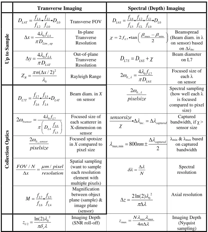
Table 2-1 LF-OCT Optical Design Considerations ... 29
Table 2-2 Summary of LF-OCT Optical Design Parameters ... 41
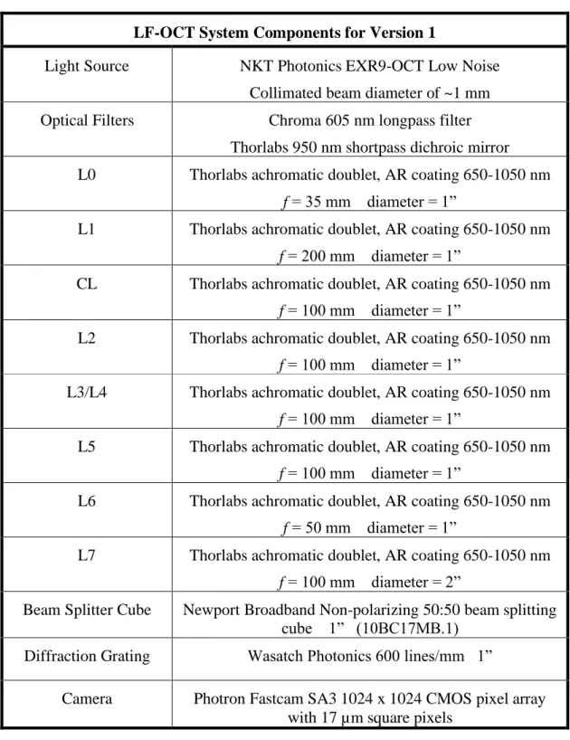
Table 2-3 Summary Components Used in LF-OCT System Version 1 ... 42
Table 2-4 Theoretical Values of Optical Design for LFOCT Version 1 ... 43
Table 2-5 Summary Comparing Performance of LF-OCT System, Versions 1 & 2 ... 64
Table 2-6 Summary of Optical Components Used in LF-OCT System, Version 1 & 2... 65
Table 2-7 Summary of SNR and Phase Resolution for LFOCT Versions 1 and 2... 66
Table 3-1 Summary of Optical Components used in LF-OCT system Version 1-3 ... 91
Table 3-2 Summary of System Performance of LF-OCT Version 1-3 ... 94
Table 3-3 Summary of SNR and Phase Resolution for LFOCT Versions 2 & 3 ... 94
Table 4-1 Frame-by-Frame MMOCT Imaging Parameters ... 125
Table 4-2 Summary of Data Reduction Metrics ... 130
Table 4-3 Imaging Parameters for Testing Effect of Temporal Sampling ... 141
LIST OF FIGURES
Figure 2-1 Schematic diagram of SD-OCT. ... 10
Figure 2-2 Illustration of A-line reconstruction in SD-OCT. ... 15
Figure 2-3 Schematic diagram of LF-OCT vs. point-scanning OCT. ... 22
Figure 2-4 Schematic diagram of the LF-OCT system setup. ... 29
Figure 2-5 Transverse vs. Spectral Planes after Cylindrical Lens. ... 32
Figure 2-6 Illustration of High-NA vs. Low-NA Focusing. ... 34
Figure 2-7 Diagram of a Transmission Diffraction Grating. ... 35
Figure 2-8 Illustration of Diffraction Grating Setup in LF-OCT System. ... 37
Figure 2-9 Ray Tracing Diagram to Determine Limiting Aperture. ... 38
Figure 2-10 Schematic Diagram of LF-OCT Setup with He-Ne laser co-aligned. ... 48
Figure 2-11 Photos of Aberrations on Shear Plate Interferometer. ... 49
Figure 2-12 Sample Arm Setup. ... 51
Figure 2-13 Comparison of B-mode Images before & after Dispersion Compensation. ... 53
Figure 2-14 LF-OCT transverse calibration of Version 1. ... 54
Figure 2-15 Axial calibration curve for LF-OCT System Version 1. ... 55
Figure 2-16 SNR vs depth for LF-OCT System Version 1. ... 57
Figure 2-17 Image of Point Scatterers for Resolution Measurement... 58
Figure 2-18 Normalized Spectra of the two SC sources. ... 61
Figure 2-19 Summary of Characterization of LF-OCT System Version 2. ... 62
Figure 2-20 B-mode Images of Ciliated hBE Cells. ... 69
Figure 2-21 Spectral Analysis of Beating Cilia with LF-OCT. ... 70
Figure 2-23 Photothermal Heating in Median Frequency Maps. ... 73
Figure 3-1 Illustration of the principle of MMOCT. ... 78
Figure 3-2 MMOCT Image Processing Steps. ... 80
Figure 3-3 Ratio of measured MNP displacement to theoretical displacement. ... 86
Figure 3-4 SNR vs depth for LF-OCT System Version 3. ... 93
Figure 3-5 Fixed Pattern Noise Correction in Photron Camera SA1.1. ... 97
Figure 3-6 Effect of Magnet Geometry on Magnetic Field Gradient. ... 101
Figure 3-7 Illustration of LF-MMOCT Sample Setup. ... 102
Figure 3-8 Photos of solenoid winding. ... 103
Figure 3-9 Comparing Solenoid Performance with Prediction. ... 106
Figure 3-10 Magnetic Field Maps of Solenoid. ... 107
Figure 3-11 2D Map of Axial Magnetic Gradient Force Delivered by the Solenoid. ... 108
Figure 3-12 Frequency Response of the Inductive Phase Lab. ... 111
Figure 3-13 Frequency Response of B-Field Amplitude. ... 112
Figure 3-14 Flowchart of MMOCT signal processing algorithm. ... 116
Figure 4-1 Fe Sensitivity of Line-by-Line and Frame-by-Frame MMOCT... 128
Figure 4-2 TEM images of magnetotactic bacteria. ... 133
Figure 4-3 MMOCT images of magnetotactic bacteria. ... 134
Figure 4-4 Magnetic SNR from MMOCT of magnetotactic bacteria. ... 135
Figure 4-5 Measuring the Fe sensitivity of the LF-MMOCT System. ... 139
Figure 4-6 Magnetic SNR vs. Temporal Sampling. ... 142
Figure 4-7 Magnitude of DFT as a function of temporal sampling. ... 145
Figure 4-9 LFMMOCT Optimal Imaging Parameters for Magnetic Sensitivity. ... 149
Figure 4-10 Magnetic Signal Map from Volumetric LFMMOCT. ... 151
Figure 4-11 VSM Data for characterizing magnetic microspheres. ... 154
Figure 4-12Stress vs Strain Curves for measuring the Young’s modulus of agarose... 155
Figure 4-13 Theoretical vibration amplitude map for point particle imaging. ... 156
Figure 4-14 LFMMOCT Images of magnetic point particles. ... 158
LIST OF ABBREVIATIONS
ALI Air/liquid interface AR Anti-reflective
CBF Ciliary beat frequency CCD Charge-coupled device
CMOS Complimentary metal-oxide semiconductor COPD Chronic obstructive pulmonary disease DFT Discrete Fourier transform
FF-OCT Full-field optical coherence tomography FPN Fixed pattern noise
FOV Field of view
FWHM Full-width half-maximum GUI Graphical user interface hBE Human bronchial epithelial IFT Inverse Fourier transform IR Infrared
LF-OCT Line-field optical coherence tomography
MCOCT Molecular contrast optical coherence tomography MMOCT Magneto-motive optical coherence tomography MNP Magnetic nano-particle
MRI Magnetic resonance imaging NA Numerical aperture
OCT Optical coherence tomography OPD Optical path delay
OPL Optical path length PCL Periciliary layer PDMS Polydimethylsiloxane
PSF Point spread function RIN Relative intensity noise
SD-OCT Spectral-domain optical coherence tomography SNR Signal-to-noise ratio
SPIO Superparamagnetic iron oxides STD Standard deviation
CHAPTER 1 -MOTIVATION
Optical Coherence Tomography (OCT) is a biological imaging modality developed in 1991 [1] as a way to perform “optical biopsies” [2] which could potentially replace the need for tissue excision or could help guide surgical biopsies. OCT produces cross-sectional images of biological tissue with a penetration depth of a few millimeters and a resolution of a few microns, placing it between microscopy and ultrasound on a size scale. Where microscopy can image at the cellular level, and ultrasound, among other biomedical imaging modalities, can image whole organs, OCT is uniquely suited for imaging at the size-scale between individual cells and organs: at the tissue scale. OCT performs cross-sectional imaging by detecting the magnitude and echo time delay of light backscattered from optically turbid media. Optically turbid means that the index of refraction of the material is spatially varying on the size-scale of the imaging
wavelength. OCT can directly image various biological tissues such as skin, airways, and eyes. OCT can also be used for distinguishing features which have similar optical properties as their surroundings (e.g. index of refraction and scattering coefficient) if a contrast agent is used. The field of molecular contrast OCT (MCOCT) consists of the various methods of contrasting molecules or molecular processes that are otherwise indistinguishable from their surroundings. MCOCT methods include both direct methods wherein the contrast agent augments or attenuates the backscattered light and indirect methods wherein the contrast agent indirectly modulates the OCT signal [3].
then applying a sinusoidally varying magnetic field, OCT can detect the resultant periodic phase shift produced by the deformation of the elastic, optically scattering medium mechanically coupled to the magnetic nanoparticles. This technique, known as Magneto-Motive OCT
(MMOCT) was developed by Amy L. Oldenburg in 2005 initially as a form of MCOCT capable of imaging magnetically-labeled macrophage cells [4], and was later demonstrated in vivo to detect the uptake of magnetite nanoparticles in tadpole livers after the tadpoles had been immersed in a tank containing magnetic nanoparticles [5]. The first MMOCT imaging tracked the periodic change in the amplitude of the light back-scattered by the scattering medium, caused by the induced motion of magnetic nanoparticles mechanically coupled to it. The technique was improved upon by tracking the periodic change in the optical phase of the OCT signal, a much more sensitive measurement than merely tracking the amplitude [6–8]. After the initial period of development, that same MMOCT technique was used to image a wide variety of biological samples without significantly changing the imaging setup or the processing algorithm: rat mammary tumors ex vivo [7], in vivo mouse eye [9,10], blood clots in ex vivo porcine arteries with magnetically-labeled platelets [11,12], blood clots in ex vivo rabbit arteries with magnetic micro-spheres [13,14], and in vivo detection of targeted magnetic nano-particles in rat breast-cancer tumors [15].
properties of biological tissues (e.g. contrasting magnetically labeled platelets in blood clots). This dissertation investigates a novel MMOCT application: to image naturally occurring magnetic particles in biological tissues.
The ability to detect and spatially locate magnetic nanoparticles is of increasing interest to biologists who study geomagnetic navigation. Many species of animals (spanning multiple classes of animals including mammals, fish, birds, and reptiles) are known to sense the Earth’s magnetic field and to use this information to navigate. One particularly puzzling example is studied by our collaborator in the Biology Department, Kenneth J. Lohmann: loggerhead turtles are able to navigate from their nesting grounds to the ocean upon first hatching, and they then travel thousands of miles through dark, seemingly featureless water in order to return years later to their original nesting grounds [21–23]. Their navigation is well correlated with perception of the Earth’s magnetic field; however, the mechanism by which turtles sense the Earth’s magnetic field remains a mystery.
There are three hypotheses currently established for potentially explaining sea turtles’ magnetic perception: 1) electromagnetic induction, 2) chemical magnetoreception, and 3)
magnetoreception. The third hypothesis is that biomineralized magnetite crystals (Fe3O4) are naturally occurring in some animals. These magnetic particles could physically rotate as the animal passes through a changing magnetic field. This hypothesis is supported by certain species of anaerobic bacteria that are known to contain chains of Fe3O4 crystals and to use these chains of paramagnetic crystals to orient themselves in the absence of light [29]. Because sea turtles also spend some of their time during migration deep under water (in the absence of light) like the magnetotactic bacteria and because they are not known to contain electroreceptors, the magnetite is the most promising theory to explain how animals like sea turtles are able to sense the Earth’s magnetic field. To test this hypothesis, we need the ability to detect and spatially locate potential magnetoreceptors embedded somewhere within the body of a sea turtle. Because sea turtles are endangered, the search would only be conducted on excised tissue taken from naturally deceased animals.
Endogenous magnetite detection poses several unique challenges. For one, the
magnetoreceptors are potentially isolated, single magnetite crystals. The size of the magnetite crystals found in the bacteria is ~50 nm in diameter, and they form single chains with lengths of ~ 1 µm [29]. The small amount of Fe contained in such potentially small magnetite crystals which may be present in a sparse distribution requires high magnetic sensitivity to be able to detect the induced periodic phase shift above the phase noise of the light coherently
(depending on the constraints of the application and commercial availability). In contrast, the concentration and size of endogenous magnetite is fixed so we have to design an MMOCT system that is sensitive to single magnetic particles with diameters at or below the OCT system resolution.
In addition to the requirement of high magnetic sensitivity, we require a high volumetric throughput so that large quantities of tissue can be imaged in a reasonable amount of time because the location of the magnetoreceptors is not known a priori and because sea turtles are large compared to the size of animals and samples previously imaged with MMOCT. MMOCT has been used to image whole, small animals (tadpoles and small fish) or small regions of larger animals. Although microscopy is able to resolve nanoparticles with a diameter of 50 nm, it may require staining to contrast the Fe and microscopy has such limited throughput that it is not a practical technique to use for this “needle in a haystack” problem. Conversely, Magnetic
Resonance Imaging (MRI) can image large bodies relatively quickly and is very sensitive to small amounts of Fe, but the spatial resolution is too coarse to allow the detection of single magnetic nanoparticles with diameters of ~50 nm when averaged together with the non-magnetic tissue in the rest of the relatively large resolution volume. MMOCT is an imaging modality uniquely suited for addressing the challenges of endogenous magnetite detection in large animals because the spatial resolution of the OCT system is on the order of ~1 µm but with a much higher throughput compared to microscopy.
optical scattering properties (which in turn affect the SNR of the recorded images), and any phase-noise contributed by the sample (e.g. due to sample motion during imaging). In this dissertation, we focus only on the imaging system’s properties as these are more readily
controlled. The sensitivity of an MMOCT system to single magnetic particles is determined by the OCT system resolution, the optical signal-to-noise ratio (SNR), and the ability to deliver sufficient magnetic force to the particle. We note that here and in the rest of this dissertation whenever we refer to “resolution” we refer to the spatial resolution of the OCT system, not the MMOCT resolution (i.e. the ability to resolve two closely spaced magnetic particles). Similarly, “SNR” refers to the optical SNR of the OCT system, unless explicitly stated otherwise (e.g.
“magnetic SNR”). For the second criterion, high volumetric throughput, we require a system with a large field of view (FOV) and a fast framerate (again, this refers to the OCT system framerate and not the MMOCT system framerate). OCT systems face fundamental tradeoffs between these two aims: to have a fine resolution, the FOV must also shrink, and because SNR is proportional to exposure time, faster framerates incur SNR losses. This is especially true of conventional OCT systems, which employ a point-scanning method to mechanically scan a focused spot across the entire transverse extent of one 2D cross-sectional image. In this case, the wider the FOV, the lower the framerate. One way to relax the tradeoff in speed and sensitivity is to employ a line-field configuration rather than a point-scanning one.
recent improvements in SC sources have reduced the noise level by using higher repetition rates and minimizing pulse-to-pulse variation [31]. By combining the line-field configuration with a SC light source and an optical design which carefully balances the need for fine resolution with a large FOV, we have designed an MMOCT system optimized for single magnetic particle
detection.
This Ph.D. dissertation is organized as follows. Chapter 2 of this dissertation covers the optical design, implementation, and characterization of our LF-OCT system employing a SC source. To demonstrate the combination of high speed, high sensitivity, and high resolution, images recorded of beating cilia on in vitro human bronchial epithelial cells are shown. Chapter 3 is devoted to the design and implementation of the hardware and software necessary to convert the LF-OCT system to the LF-MMOCT system. This chapter also covers the theory of MMOCT and the characterization of the system hardware. In Chapter 4, the development of a new
CHAPTER 2 -DEVELOPMENT OF LINE FIELD-SD OCT SYSTEM
As previously mentioned, OCT is a well-established biomedical imaging modality that produces 2D cross-sectional images from optically turbid media. The principle of OCT is low coherence interferometry [32] (coherence, in this case, referring to temporal coherence). The most widely used form of OCT is Spectral-Domain OCT (SD-OCT). In this chapter, I will give only a brief overview of SD-OCT since this theory has been extensively covered in previous works [33–35]. Next, I will discuss how SD-OCT theory is applied to line-field systems. By examining expressions for SNR in traditional SD-OCT and in LF-OCT, I will demonstrate why we are able to relax the fundamental tradeoff in speed and sensitivity inherent in SD-OCT systems by using the line-field configuration.
In Section 3, I will describe the optical design considerations for a LF-OCT system, the choice of optical elements for Version 1 of our LF-OCT system, the alignment procedure and the characterization of that system. Then I will discuss how the performance of Version 1 of the LF-OCT system informed the changes we made in the optical design to produce Version 2. Lastly, in Section 4, the LF-OCT system’s high-speed, high sensitivity, and high resolution are
demonstrated by imaging beating cilia on human bronchial epithelial (hBE) cells in vitro.
2.1 SD-OCT theory
destructively depending on the optical path delay (OPD) of the two beams. Importantly, the phenomenon of interference can only occur if the OPD is within the coherence length of the light source. Temporal coherence is analogous to the “memory” of the light. If the OPD between the beams is too large, then it is as if they no longer have any memory of the other when they recombine, and they will not interfere. If, however, the OPD is less than the coherence length, then the two beams retain some “memory” of each other and will interfere when recombined. The coherence length, lc, (defined as the length over which the magnitude of the light source’s
temporal coherence function has dropped to 1/e) is given by equation 2-1:
2 0
c
l
=
(2-1)
where λ0 is the center wavelength, Δλ is the full width at half maximum (FWHM) of the source
power spectrum, assuming a Gaussian emission spectrum. From this equation, it becomes clear that for a monochromatic source, the bandwidth is infinitely small so that the coherence length is infinite. This is why the temporal coherence is related to how monochromatic the light is;
broadband light is by definition light with low temporal coherence. OCT is a form of low-coherence interferometry since it employs broadband light.
Commonly, SD-OCT systems use a Michelson interferometer: the incident polychromatic (meaning broadband spectrum) plane wave, with an electric field that can be expressed as Einc =
s(k, ω)ei(kz-ωt), is split into a reference beam, E
R(k, ω) and a sample beam, ES(k, ω) (see Figure
2-1). In this expression, s(k, ω) is the electric field amplitude as a function of the spatial and temporal frequencies of each spectral component characterized by a wavelength, λ, and a
Figure 2-1 Schematic diagram of SD-OCT.
Schematic diagram of basic SD-OCT setup consisting of a broadband light source, a Michelson interferometer and a spectrometer. If the OPD between the two arms is within one coherence length, the recombined light exhibits interference. The recorded spectrum of the interference
output carries a spectral modulation as a function of the OPD.
The light exiting the beam splitter, after having been reflected from the reference arm mirror and the scattering object in the sample arm, is recorded by a spectrometer composed of a diffraction grating and a camera. The camera records the intensity of the combined light, ID, which is
proportional to the square of the total field:
2
( , )
2
D
k
E
RE
SI
=
+
(2-2)where ρ is the responsivity of the detector, the factor of ½ accounts for the power lost by passing through a 50:50 beam splitter, and the angular brackets denote averaging over the response time of the detector. The polychromatic plane waves in the reference and sample arms are reflected or backscattered by the reference mirror and the scatterers in the sample arm, respectively. The reference arm mirror is characterized by an electric field reflectivity, rR, and the distance from
square of the complex field amplitude, the power reflectivity, RR, is given by RR = |rR|2. Likewise,
the scatterers in the sample arm are characterized by their field reflectivities, rSi, power
reflectivities, RSi, and distance from the beam splitter, zSj. Following the derivation in Ref [32],
we can now write out a more explicit form of equation 2-2, assuming a series of N discrete, real, delta-function reflections from the sample:
(
)
22 ( )
(2 ) R
1
( , )
( , )
( , )
e
e
2
2
2
SS Sj SS
R
N
i k z n z z t i kz t
D Sj
j
s k
s k
I k
r
−
r
+ − −=
=
+
(2-3)where n is the refractive index of the sample, and zSS is the distance from the beam splitter to the
sample surface. Expanding the squared term in equation 2-3, we can write out the three terms that contribute to the detected intensity:
1
( )
( )
4
N
D R Sj
j
I
k
S k
R
R
=
=
+
(
2(
( ))
2(
( ))
)
1
( )
e
e
4
R SS Sj SS R SS Sj SS
N
i k z z n z z i k z z n z z R Sj
j
S k
R R
− − − − − − − =
+
+
2 ( ) 2 ( )
1 1
( )
(e
e
)
4
Sm Sj Sm Sj
N N
i kn z z i kn z z Sm Sj
m j m
S k
R R
− − −= =
+
+
(2-4)In this expression, s k( , )
2 is written as S(k), the power spectral density of the light sourceused in OCT. The first term has no dependence on the location, zS, of the scatterers. This is
usually called the “DC” term because it has no modulation in k, and it can be subtracted out of
the OCT signal in post-processing. Generally, OCT images are collected with the sample arm and reference arm powers adjusted such that RR is much larger than RS (and biological tissues are
generally weakly scattering with RS << 1). In this case, the DC term dominates ID. The second
term is the cross-term. This is the term that contains useful information about the location of scatterers within an image because this term depends on the OPD between each scatterer and the fixed reference arm. For every scatterer in the sample arm, there is a corresponding contribution to the cross-term. The third term is called the auto-correlation term because it comes from the interference of light backscattered from scatterers at different depths in the sample.
The goal of OCT is to reconstruct the field reflectivity of the sample as a function of depth within the sample, rS(z). This reflectivity profile is what constitutes the structural images
produced by OCT. To reconstruct the field reflectivity profile of the sample from the recorded spectral intensity, we make use of the Wiener-Khintchin theorem which says that the power spectral density is equal to the Fourier transform of the temporal autocorrelation of the electric field. We have recorded the spectrum using a spectrometer. This spectrum carries a spectral modulation with a period (in wavenumber) given by 2π divided by the OPD between the sample and reference arms, 2π/2[zR–zSS – n(zsj –zSS)]; each scatterer j at some depth zSj is characterized
by its own spectral modulation frequency, with an amplitude scaled by its reflectivity rSj, and the
modulated spectrum is a superposition of all the modulation frequencies. Now, we take an inverse Fourier transform (IFT) of ID(k) from equation 2-4 to reconstruct the field reflectivity
1
( )
( ( ))
8
N
D R Sj
j
I
z
IFT S k
R
R
=
=
+
(
)
1 ( ( )) ( ) ( ) 4 NR Sj j j
j
IFT S k R R z z z z
= + + + −
(
)
1 1 ( ( )) ( ) ( ) 8 N NSm Sj Sjm Sjm
m j m
IFT S k R R z z z z
= =
+ + + −
(2-5)where Δzsjm = 2n(zSj-zSm) is the optical path delay between two scatterers located at depths zSj and
zSm within the sample and Δzj = 2(zR – zSS – n(zSj – zSS)) is the optical path delay between the
reference mirror and a scatterer located at a depth zSj in the sample.
Recall our initial assumption that the scatterers were a series of real, delta functions. We have now reconstructed these delta functions using the fact that the Fourier transform of a cosine function (re-writing the exponentials in equation 2-4 in terms of a cosine via Euler’s rule) is a pair of delta functions. However, these delta functions are now broadened due to the convolution with the coherence function of the light source, IFT(S(k)). Assuming a Gaussian emission
spectrum both for convenience and because most light sources used in OCT typically have approximately Gaussian spectra, with bandwidth Δk, and wavenumber of center wavelength, k0,
we can write the coherence function of the light source as follows:
2 0 ( ) ( )
1
( )
z
IFT S k
( ( ))
e
z ke
izk
− −=
=
(2-6)The complex exponential in equation 2-6 will drop out if we take the absolute value of the inverse Fourier transform (as in Figure 2-2), and is sometimes excluded from expressions of
ID(z). By convolving the coherence function with the delta functions, we reconstruct the sample’s
(the RR component of the DC term in equation 2-5) and assumed that the autocorrelation terms
are small enough to be negligible. The reference term, ID(k)ref, is subtracted by recording one or
more images with nothing in the sample arm, averaging those frames (if applicable), and then subtracting this reference frame from each spectral interferogram. The assumption that the autocorrelation terms are small is justified by the way that the power is adjusted in the reference and the sample arms. Typically, the reflectivity of scatterers in the (biological) samples, rS, is
small compared to the reflectivity of the reference arm mirror, rR, so that RR dominates the
detected intensity, ID(z). And, in fact, the ratio of reference to sample arm power is an important
consideration for setting up an OCT system to image a particular sample; the sample must be illuminated with sufficient power such that the scatterers are detectable above the noise of the system without using so much sample power that the autocorrelation terms become problematic. The reference arm power is then adjusted so that the maximum amount of light is collected by the sensor without saturating it. A simplified expression for the reference-subtracted OCT signal is given in equation 2-7:
(
)
2 2(
)
(
)
2 2(
)
0 0
1
( )
4
j j j j
N
z z k i z z k z z k i z z k
OCT R Sj
j
S
z
R R
e
− + e
− +e
− − e
− −=
+
(2-7)The two sets of exponentials in equation 2-7 represent an important aspect of OCT: a scatterer located at an OPD +Δz from zR and a scatterer located –Δz from zR will produce
identical OCT signals. In order to avoid confusion or wrapping effects in the structural OCT image, we choose to set up the sample arm such that all scatterers are on the same side of the plane z = zR. The mirror image produced in the region zR – Δz is called the conjugate image and is
reconstruction. In fact, the delta functions are all broadened by the coherence length of the coherence function. To better resolve the peaks in rS(zs), a light source with a shorter coherence
length should be used; this is why broadband sources are used for high-resolution imaging in spectrometer-based OCT. Each depth profile is called an A-line. If the beam in the sample arm is scanned across the surface of the sample, then we can build up an array of depth profiles and thereby create one 2D cross-sectional image, called a B-mode image.
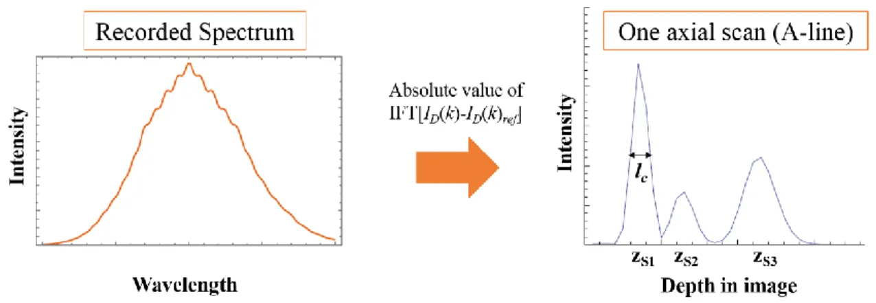
Figure 2-2 Illustration of A-line reconstruction in SD-OCT.
The spectral interferogram of the light recombined from the reference and sample arms carries a spectral modulation as a function of OPD between the reference mirror and each scatterer in the sample. Taking the absolute value of the IFT yields a reflectivity profile for one
transverse location on the sample surface; each depth profile is called an A-line.
The axial resolution, Δz, is then given by the coherence length of the light source, and is typically defined in terms of the FWHM, rather than the 1/e width as in equation 2-1, of the temporal coherence function (the temporal autocorrelation function of the electric field of the light source). For a Gaussian emission spectrum, the FWHM is given by:
2 0
2 ln 2
z
n
=
where n is the refractive index of the sample and λ0 and Δλ are the source center wavelength and
bandwidth, respectively. Importantly, the axial resolution in OCT is completely decoupled from the focusing optics, so a high axial resolution can be achieved independently of the sample arm objective lens used.
In traditional SD-OCT systems, the light is focused into a spot on the sample surface. The transverse resolution is given by the FWHM of the Gaussian intensity profile as a function of radial distance from the optical axis. For a Gaussian beam, assuming the incident beam is collimated so that the focused beam waist occurs a distance f away from the lens and that the divergence angle of the focused Gaussian beam is small (2θ ~ d/f), the transverse resolution, Δx, is given by:
0
4
f
d
x
=
(2-9)where f is the focal length of the sample arm objective lens and d is the beam diameter on that lens [36]. This is called the diffraction-limited spot size, and is the same expression used in microscopy.
The axial ranging capabilities of OCT and the relatively large imaging depth are the primary differences between OCT and confocal microscopy. Several factors influence the maximum depth that can be imaged with OCT. The first major consideration is the limited spectral resolution of the spectrometer, the effect of which can be modeled by an optical SNR fall-off in depth. The depth at which the detected intensity falls off by ½ can be written:
2 0 1/ 2
ln(2)
r
Z
where ∂rλ is the spectral resolution of the spectrometer. The second major consideration for the maximum imaging depth in SD-OCT is how the spectral interferogram is sampled. Although the spectrum is continuous, it is sampled by a finite number of pixels. Recall that each A-line (depth-dependent reflectivity profile) is obtained by taking a Fourier transform of the modulated
spectrum. The maximum depth that can be imaged is limited by the Nyquist sampling theorem, which gives the number of discrete samples needed to capture all the information contained in a continuous signal of finite bandwidth. The bandwidth of the broadband light source (after being spread by a diffraction grating) is sampled by N pixels, giving a wavelength sampling δsλ =
Δλ/N. We can write the maximum, one-sided imaging depth achievable by a spectrometer in terms of the bandwidth captured by the spectrometer, Δλ, the number of pixels, N, and the sample’s refractive index, n:
2 0 max
4
N
Z
n
=
(2-11)Both Z1/2and Zmax can be limiting factors for the practical imaging depth achievable by an OCT
system; however, Zmax is typically the figure of merit used in SD-OCT publications as the
imaging depth. One reason for this is that while the number of pixels is fixed by the sensor used, the sensitivity roll-off dictated by equation 2-10 can be mitigated by appropriately designing the spectrometer focusing optics, as it has been shown that the spot size of the beam on the
NIR region, the imaging depth achievable in most biological tissues is limited to ~ 2mm by the scattering properties of the tissue itself [35]: scattering in biological tissues is primarily in the forward direction [39], which limits the number of mean free paths that can be imaged in depth due to multiple scattering, and sub-resolution sample heterogeneities give rise to further multiple scattering events, which is ultimately the most limiting factor for OCT imaging depth [40].
The final key parameter governing the performance of an SD-OCT system is the signal-to-noise ratio (SNR), which we use interchangeably with “sensitivity” throughout this
dissertation. The SNR is a measure of the smallest amount of back-scattered light from a single coherence volume that can be distinguished from the background noise. For low-coherence interferometry, the SNR is defined as the ratio of the mean-squared OCT signal (equation 2-7) and the variance of the noise [31,41]:
2
2 OCT
noise
S
SNR
(2-12)From equation 2-2, the mean-squared OCT signal is proportional to the absolute square of the electric fields ER and ES. Because optical power is proportional to the square of the field, the
mean-squared OCT signal is proportional to the product of the sample arm power and the
reference arm power, PR·PS. The noise, σnoise2, is given by the variance of the mean-squared OCT
signal in regions of low backscattering and can be classified into three categories:
2 2 2 2
det
noise ector shot excess
=
+
+
(2-13)semiconductor (CMOS) sensor [42]. However, the most important consideration for this dissertation is the dependence on the power. The detector noise, σ2
detector, has multiple
components, most of which boil down to random fluctuations in the sensor electronics caused by thermal noise [41,43,44]. The detector noise is independent of the reference arm power. Shot noise, σ2
shot, is a result of the quantum mechanical nature of light and the Heisenberg uncertainty
principle. Shot noise is proportional to the reference power (recalling our assumption that the power exiting the reference arm is much greater than that of the sample arm) [42,43,45,46]. The third term, σ2
excess, is photon excess noise caused by photon bunching. The exact form depends
on the light source used but is proportional to the square of the reference arm power [47]. In the shot-noise limited regime (i.e. without photon excess noise), the SNR in decibels can be written:
10
2
10*
P
Aline AlineT
SNR
h
Log
=
(2-14)where η is the quantum efficiency of the detector, PAline is the power in a single A-line incident
on the sample, T is the exposure time of the detector for a single A-line, and hν is the energy of the center wavelength of the light source [41]. For flying-spot OCT, the power per A-line is the total power in the sample arm because the entire beam is scanned over each transverse position, and the exposure time is 1/linerate of a linescan camera.
The quantum efficiency of the detector, η, is determined by the choice of camera and the energy of the center wavelength is determined by light source. For a given SD-OCT system, these are fixed parameters. This means that for a given line rate, the only way to improve the SNR is to increase the sample power. However, the sample power cannot be arbitrarily increased without bound. For example, every light source has a maximum power output, and for typical broadband light sources used in SD-OCT, the maximum power output is a few hundred mW. More importantly, because OCT is a biomedical imaging modality, safety standards must be taken into consideration. For continuous-wave laser illumination of biological tissues, the figure of merit for damage thresholds is the peak irradiance of the light (i.e. the maximum power per unit area illuminated by the laser) [48]. For typical SD-OCT systems, the light at the sample is focused into a spot at the surface of the sample. Because the illuminated area is so small, the maximum power that can safely be used is limited.
One way to relax the fundamental tradeoff in speed and sensitivity inherent in SD-OCT while maintaining a safe intensity is to parallelize the detection. Two methods currently
detection is line-field OCT, a spectrometer-based technique that offers sensitivity advantages with slightly more coarse transverse resolutions.
2.2 LF-OCT theory
Line-field OCT (LF-OCT) is a form of OCT in which the light in the sample arm is focused into a line rather than a spot at the surface of the sample. The spectral interferogram is then recorded on a 2D pixel array rather than a line scan camera, with one dimension being the wavelength and one dimension of the pixel array recording the transverse position. In this way, all A-lines are recorded simultaneously and we can reconstruct a 2D B-mode image from one camera frame without the need for mechanical scanning. These differences are illustrated in Figure 2-3.
It is immediately obvious that the line-field configuration presents a factor of N
improvement in speed (N being the number of transverse A-lines recorded in a B-mode) because
N A-lines can now be recorded during the same exposure time, T, that previously each A-line required. Additionally, because the sample power is spread across many A-lines, a higher total sample power can be used without damaging the tissue. This means that we can re-write the expression for SNR from equation 2-14 with a total sample power PS that is N times higher than
the power per A-line, PAline:
10
2
10*
AlineLF
P
NT
SNR
h
Log
=
(2-15)photothermal heating has not been well characterized yet for line-field systems; the heat dissipation may be less effective in a light-sheet geometry than in point-scanning systems.
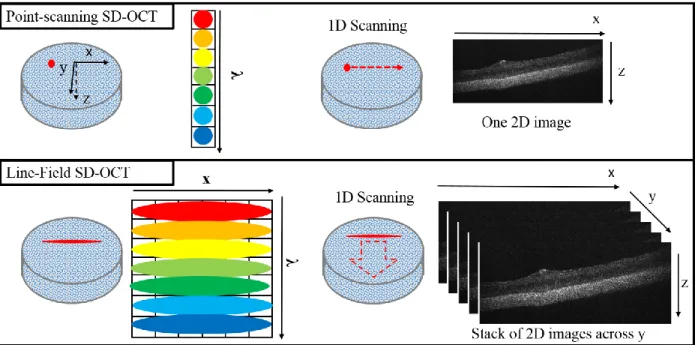
Figure 2-3 Schematic diagram of LF-OCT vs. point-scanning OCT.
Top panel: point-scanning SD-OCT employs a mechanically scanned focal spot at the sample and a 1D line-scan camera. Mechanical scanning is required to produce each 2D B-mode image. Bottom panel: line-field SD-OCT employs a line illumination at the sample and a 2D pixel
area-scan camera so that a 2D B-mode image is formed without any mechanical area-scanning.
quantity (which is the measure of phase stability typically used in the literature) is the phase resolution, δθ [51,52]. The phase resolution is considered the smallest phase change that can be reliably detected by a given system, and it is related to the SNR as follows [52]:
1
( S, , s)
SNR P T R
= (2-16)The dependence of the SNR on the total sample power, exposure time, and reflectivity of the scatterer is shown. (Rs assumed to be 1 in equation 2-15, as this value is typically measured from
mirrors and other nearly perfect reflectors.) The associated uncertainty in the displacement of a scatterer is then given by:
0
4
z
n
=
(2-17)From Figure 2-3, it is also clear that the focusing of the beam onto the sensor in the X
dimension is different in point-scanning and line-field OCT. In point-scanning OCT, the resolution in both X and Y is given by the same expression for the beam waist of a Gaussian beam, equation 2-9. This expression is the same for the out-of-plane resolution, Δy, in LFOCT. However, the in-plane transverse resolution, Δx, is determined by the ability of the collection optics (the series of lenses downstream from the sample) to focus light scattered by a point-particle onto the sensor. A more detailed explanation of how to calculate Δx requires an understanding of the LFOCT system setup, so it is reserved for after a description of the collection optics is given at the end of Section 2.3.1. The expressions for axial resolution and imaging depth remain the same for LFOCT systems.
the sample power is now spread across all A-lines so there is up to a factor of N improvement to speed. This means that if light sources exist which offer higher power over the wavelength ranges typically used in OCT, line-field OCT can offer a higher speed with a comparable SNR, thereby relaxing the tradeoff in speed and sensitivity.
Supercontinuum (SC) light sources are promising for high-power, broadband light sources for LF-OCT. A nonlinear optical process involving a photonic crystal fiber produces an ultrabroad bandwidth spectrum with more power than conventional OCT light sources.
Historically, SC sources have been very noisy, making them unsuitable for OCT imaging
because of the loss of SNR [53,54]. SC sources suffered from excess photon noise, meaning that they could not be operated in the shot-noise limited regime. In the shot-noise limited case, the SNR can be increased by increasing the power incident on the sample. When excess photon noise dominates, increasing the sample power does not result in increased SNR. However, recent advances in SC technology have produced lower noise sources suitable for OCT. In 2014, Brown
significantly more power than the super luminescent diodes and femtosecond lasers typically used in OCT.
2.3 Optical Design of a LF-OCT System
2.3.1 Optical Element Selection
The key optical element for LF-OCT systems is the cylindrical lens. Unlike spherical lenses which focus light into a circular spot by focusing in both planes orthogonal to the optical axis (referred to as the X and Y planes throughout this chapter), a cylindrical lens focuses a collimated input beam in only one transverse plane of the optical axis while the beam remains collimated in the other transverse plane. This produces a line illumination at the focal plane of the lens. The length of the line illumination is characterized by the 1/e fall-off in intensity of the Gaussian irradiance profile.
The introduction of the cylindrical lens adds a significant degree of complexity to the optical design of an OCT system, primarily due to the fact that 1) there are now twice as many design parameters to consider because the two transverse planes must be treated separately, and 2) the beam must now be significantly enlarged compared to the beam diameters typically used in OCT systems because the transverse FOV (i.e. the size of the line illumination at the sample) is determined by the collimated beam diameter (in the plane defined as X in Figure 2-3) output by the lens immediately before the sample. (This is different from point-scanning SD-OCT systems where the desired FOV is set by the sweep range of the mechanically scanned focused spot.) A large beam diameter is also desirable in LFOCT for achieving a fine transverse
possibility of beam clipping on an optical element is high. Further, after passing through the cylindrical lens, the beam has a different diameter in the two transverse planes, X and Y, thus doubling the number of parameters that must be considered.
To begin any design, the first consideration is the application because this dictates what the figures of merit of the design are. The ultimate purpose of this LF-OCT system is the
resolution volume; this means that the optical phase we measure is a kind of weighted average (weighted by the reflectivity) of the phase shifts from every backscattered photon within one resolution volume. In the condition that the particle volume is much smaller than the resolution volume (as in the case of 50 nm diameter magnetite crystals with typical OCT resolution volumes), the larger the spatial resolution, the smaller the difference in the measured optical phase shift compared to stationary, neighboring resolution volumes. The relationship between the size of the resolution volume and the detectable displacement of a magnetic nanoparticle is discussed further in Chapter 3.
The second requirement of the LFOCT system for endogenous magnetite detection is high throughput, which we define here as the volume of tissue imaged per second (expressed as mm3/s). High throughput is achieved by imaging as large a volume as possible and as quickly as possible. The volume of tissue imaged by a single B-mode is given by the product of the
spectrometer). With a fixed number of data points, one cannot get information over an infinitely big area with an infinitesimally small resolution. So in general, in optical imaging systems such as OCT or microscopy, the bigger the transverse FOV, the coarser the resolution. Given these two sets of tradeoffs, we see that there is a fundamental tradeoff between the ability to detect single magnetic particles (with volumes less than the resolution volume) and the volumetric throughput of the imaging system. The optical design must carefully balance these tradeoffs, with the decision being made to favor the ability to detect single magnetic particles over volumetric throughput if we have to choose one or the other.
Table 2-1LF-OCT Optical Design Considerations
Fixed Parameters Design Goals Fundamental Tradeoffs
Initial Beam Diameter
Achieve desired transverse FOV and Δx/Δy at sample
Small Δx & Δy vs. large Rayleigh range Pixel Array Size Match the beam diameter in both X and λ to
the pixel array size with sufficient sampling
Small Δz vs. large imaging depth
The basic layout for the LF-OCT system is shown in Figure 2-4, and is adapted from the optical design used in [55]. The choice of each element was made as follows.
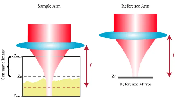
Figure 2-4 Schematic diagram of the LF-OCT system setup.
Broadband light from an NKT SC source is first filtered to a bandwidth of 300nm centered at 800nm. The beam is expanded by L0 and L1 and then enters a free-space Michelson interferometer. Light back-scattered from both arms is recombined and collected by a
The Light Source. The first version of the LF-OCT system was designed for a demo light source loaned to us by NKT Photonics. It was an EXR9-OCT Low Noise SC source made specifically for use in OCT systems. The source has a repetition rate of 320 MHz (the high repetition rate contributing to the lower noise), a beam diameter of ~1 mm at 530 nm (as reported by NKT Photonics), and the output is a collimated, single-mode Gaussian. The source emits ultra-broadband light from 400 nm – 2400 nm with a total output power of 900 mW over the visible to near infrared (NIR) range (550-900 nm).
Optical Filters. A SC source offers the unique advantage to an OCT system design that you can select the desired bandwidth to use, and by changing the optical filters used, could change the design and application of the OCT system. The bandwidth dictates the application to some extent because, as mentioned in Section 2.1, the axial resolution and imaging depth both depend primarily on the source bandwidth, Δλ, and the center wavelength, λ0. In terms of the Nyquist sampling criteria, equation 2-11, visible light OCT has a finer axial resolution, but lower imaging depth; conversely infrared (IR) OCT has a longer penetration depth but coarser axial resolution. The Nyquist sampling criteria is not the only factor governing the practical imaging depth achievable with OCT; the absorption and scattering properties of the sample itself will also serve to change the attenuation of the beam in depth. The beam attenuation is often the practical limit on the measured imaging depth. Using the Nyquist sampling criteria as a general sample-independent method for estimating the imaging depth, the bandwidth selection must weigh the benefit of high axial resolution against the corresponding cost in imaging depth. For our purposes, we desire high axial resolution, but we also need to maintain reasonably good
depth > 0.5 mm; the use of shorter wavelengths (a branch of OCT called visible light OCT) can provide even finer axial resolution but at the cost of an even further reduced imaging depth [56]. From equations 2-4 and 2-5, this corresponds to a theoretical axial resolution of 1 µm and a maximum imaging depth of 564 µm in air (for an array of 1024 pixels, assuming Nyquist sampling). Using a dichroic mirror (Thorlabs DMLP950) to reflect light with wavelengths <950 nm and a long-pass filter (Chroma ET605lp) to transmit light with wavelength >605 nm, we filter the SC source’s bandwidth down to ~350 nm. The wavelengths <605 nm and >950 nm are
directed into a beam dump. We then align the beam on the camera sensor such that only the range 650-950 nm is captured by the camera, as discussed later in this section.
First Beam Expander (L0 and L1). The choice of the first beam expanders depends on the desired transverse FOV at the sample. To understand how the length of the line illumination depends on the focal lengths chosen, see Figure 2-5. The collimated output from the first beam expander (composed of lenses L0 and L1) is incident on the cylindrical lens, CL. From the figure below, it is clear that after the CL, the beam is always focusing in one of the two planes
Figure 2-5 Transverse vs. Spectral Planes after Cylindrical Lens.
Schematic diagram illustrating how the beam in a LF-OCT system is focused in the two transverse planes after passing through the cylindrical lens, CL. The beam is always focusing in
one plane and collimated in the other.
From Figure 2-5 it is clear that the choice of lenses for the first beam expander will affect all downstream parameters, so the optical design will be an iterative process rather than a simple formula. As a starting place, we chose a FOV of ~4-5 mm. From the expression for the
transverse FOV in Table 2-2, we need a combination of four lenses (L0, L1, L2 and L4) whose combination increases the beam diameter of the collimated NKT output (measured to be roughly 0.7 mm) to 4 or 5 mm. In practice, you can make initial guesses for these four lenses and then tweak them as you fill in this chart of design parameters after choosing the downstream optical elements as well. Our choice of lenses was based in large part on which focal lengths were readily available. We used only achromatic doublets with an anti-reflective (AR) coating for the wavelength rage 650-1050 nm from Thorlabs, which limits the possible focal lengths
aberrations which is a concern when using a bandwidth as broad as 300 nm. The AR coating is essential to prevent loss of power in applications requiring high SNR. For the beta version of the LF-OCT system, called Version 1 throughout this dissertation, we chose to make the first beam expander with focal lengths fL0 = 35 mm and fL1 = 200 mm to expand the beam to 4 mm. We then used a focal length of 100 mm for lenses L2 and L4 (and L3, to match the sample and reference arms) so that the theoretical transverse FOV at the sample was 4 mm. These four lenses together also determine the theoretical out-of-plane transverse resolution we can achieve at the sample, given by the focused beam waist as in equation 2-9. With the focal length of L4 being 100mm and the beam diameter incident on it being 4 mm, the theoretical transverse
resolution is 25 µm. As stated previously, there is a fundamental tradeoff in transverse resolution and Rayleigh range. The Rayleigh range is the distance along the optical axis at which the radius of the focused beam waist of a Gaussian beam increases by a factor of the square-root of two, and is given by the following expression:
2
0
(
/ 2)
R
n
x
Z
=
(2-18)Figure 2-6 Illustration of High-NA vs. Low-NA Focusing.
Schematic diagram illustrating the inverse relationship between the focal spot, 2ω0, (1/e diameter
of a Gaussian intensity profile) achieved by a Gaussian beam and the corresponding Rayleigh range, ZR. Low NA objectives (small incident beam diameter and/or long focal length lens) focus
the beam to a larger spot size, but maintain a relatively uniform beam diameter over a longer range compared to high NA objectives which achieve a smaller focal spot but with greater beam
divergence away from the focal plane. The depth of focus, b, is twice the Rayleigh range.
Collection Optics. After considering the first five lenses which bring us up to the sample plane, the next major consideration is matching the beam diameter in both the transverse and spectral planes to the size of the camera’s pixel array. The pixel array in this system is a CMOS
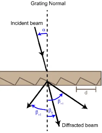
from the incident light. A transmission grating is made of a transparent optical element with a set of regularly spaced grooves carved into the surface. These grooves are spaced by a separation distance, d. When light is incident at an angle α to the grating normal, a series of diffracted beams will appear on the other side. The diffraction of light through a transmission grating is shown in Figure 2-7.
Figure 2-7 Diagram of a Transmission Diffraction Grating.
Light incident on a diffraction grating with groove spacing d and angle of incidence α is diffracted into multiple orders, with the angle of diffraction β being wavelength dependent.
The angular locations, βm(λ), of the intensity maxima are governed by the grating equation:
(sin
sin
m)
m
=
d
+
(2-19)interested in the first diffraction order, where the intensity is highest of all the diffracted beams. The grating equation can also be written in terms of the groove frequency, G = 1/d:
sin
sin
mGm
=
+
(2-20)If the diffraction grating is placed at the focal plane of L7 and if we align the beam such that the diffracted center wavelength, λ0, is orthogonal to the lens L7, as shown in Figure 2-8 below, the beamspread, χ, is estimated by the following expression:
max min
7
2 tan
2
L
f
= − (2-21)
where βmin and βmax are the found using equation 2-13, and λmin and λmax are found by
determining the actual bandwidth captured by the spectrometer (proportional to the ratio of the beamspread to the sensor size if χ is larger).
Using a transmission grating with 600 lines/mm (Wasatch Photonics 2996-12), a focal length of 100 mm for L7, and an incident angle of 13°, the 1st diffraction order beamspread, χ, on lens L7 for our chosen wavelength range is 18.6 mm. This is the size of the beam in the spectral dimension on the camera. Because this is slightly larger than the length of the pixel array, we must account for the slight cropping in the actual bandwidth Δλ recorded on the spectrometer.
Given the ratio of the array length to the beamspread, the actual bandwidth captured is 280 nm. Being sampled by 1024 pixels, this gives a spectral resolution of 0.273 nm per pixel.
7 5
6 4
L L
L L
f
f
M
f
f
=
(2-22)With fL7 = fL4, the magnification is merely the ratio of fL5 and fL6. These were chosen to be 100
mm and 50 mm respectively, yielding a magnification of 2 and a transverse extent at the sensor of 8 mm.
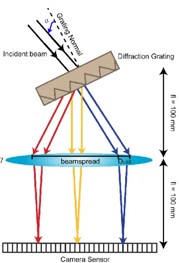
Figure 2-8 Illustration of Diffraction Grating Setup in LF-OCT System.
The diffraction grating is placed at the focal plane of L7 and at an angle such that the center wavelength λ0 = 800 nm of the first diffraction order is perpendicular to the lens L7.
discussion that the Δx is determined by the ability of the collection optics to focus light
backscattered from a point source onto the sensor. Generally, a point particle in the sample may scatter light in any direction. The OCT system can only collect light that is scattered at some maximum angle relative to the optical axis, and that angle is determined by the limiting aperture (sometimes called the aperture stop) of the system. In a multi-lens system with no obvious limiting aperture, the limiting aperture is the rim of the lens which most limits the scattering angle that can be collected [57].
Figure 2-9 Ray Tracing Diagram to Determine Limiting Aperture.
A point source in the sample may generally scatter light in any direction. The limiting aperture determines which scattering angles can be collected and imaged onto the sensor. The diagram shown here (to-scale) illustrates that the rim of lens L4 acts as the limiting aperture in
our LFOCT system (Top panel). The ray tracing of an off-axis point source (bottom panel) illustrates that our system suffers from vignetting, meaning that the extreme rays from off-axis
points are not collected and therefore the intensity of those off-axis points will suffer.
same information about limiting aperture as does ray tracing of an off-axis point; however, ray tracing of an off-axis point can provide useful information about intensity loss due to vignetting, the process by which not all the light back-scattered from off-axis points is collected resulting in non-uniformity in the transverse recorded intensity profile [57].
From Figure 2-9, we see that the diameter of the lens L4 is the limiting aperture of our LFOCT system. All the rays from an on-axis point source will be collected and mapped to the sensor as long as they are incident on the lens L4. The ability of the system to focus the light from that point source onto the sensor is then given by the expression for the focused Gaussian beam waist, as in equation 2-9, but now the focal length of the lens is the focal length of L7, and the beam diameter incident on L7 is given by the ratio of the focal lengths of L6 and L5
multiplied by the diameter of the lens L4, DL4:
0 7 0 6 4 5 4
2
L sensor L L L f f D f
=
(2-23)Given the focal lengths fL5, fL6, and fL7 of 100 mm, 50 mm, and 100 mm respectively and that L4 is a standard 1” optic (diameter of 25.4 mm), the size of the focused Gaussian beam waist is 8.02 µm at the sensor. Given a magnification of 2 between the object plane (at the sample) and the image plane (at the sensor) from equation 2-22, this results in a theoretical transverse resolution of 4.01 µm at the sample (i.e. the value for the theoretical transverse resolution in physical lab space). The full expression for the theoretical transverse resolution of the LFOCT system with the diameter of lens L4 as the limiting aperture is then the expression in equation 2-21 divided by the magnification, which simplifies to:
0 4 4