A NEW STATIONARY DIGITAL BREAST TOMOSYNTHESIS SYSTEM: IMPLEMENTATION AND CHARACTERIZATION
Jabari Calliste
A dissertation submitted to the faculty at the University of North Carolina at Chapel Hill in partial fulfillment of the requirements for the degree of Doctor of Philosophy in the
Department of Applied Physical Sciences.
Chapel Hill 2016
Approved by: Cherie Kuzmiak David Lalush Yueh Z. Lee Jianping Lu
iii ABSTRACT
Jabari Calliste: A new generation stationary digital breast tomosynthesis system: Implementation and characterization
(Under the direction of Otto Zhou)
Digital breast tomosynthesis systems (DBT) utilize a single thermionic x-ray source that moves around the breast in a fixed angular span. As a result, all current DBT system requires the mechanical motion of the x-ray source during the scan, limiting image quality either due to the focal spot blurring or a long scan time. This causes an unfavorable reduction in the in-plane resolution compared to 2D mammography.
Our research group developed and demonstrated a first generation stationary digital breast tomosynthesis (s-DBT) system that uses a linear carbon nanotube (CNT) x-ray source array. Since the stationary sources are not subject to focal spot blurring, and images can be acquired rapidly, the in-plane system resolution is improved. Additionally, image acquisition time is independent of angular span since there is no motion, allowing for large angular spans, and increased depth resolution. The improved resolution of the first generation s-DBT system over continuous motion (CM) DBT has been demonstrated with image evaluation phantoms and a human specimen study. The first generation s-DBT is currently undergoing clinical trials at the University of North Carolina Cancer Hospital.
iv
cost on patient imaging time. The goal of this thesis work was to design construct and
characterize a second generation s-DBT system, capable of faster image acquisition times, and higher depth resolution than our first generation system.
v
ACKNOWLEDGEMENTS
I would like to thank both my advisors, Dr. Otto Zhou and Dr. Jianping Lu, for their leadership, guidance and encouragement throughout my graduate studies. Being able to work with them on research that translates to useful applications today has truly motivated me. It was an absolute pleasure working with you. I also highly appreciate the rest of the members in my committee, Dr. Cherie Kuzmiak, Dr. David Lalush, and Dr. Yueh Z. Lee for their direction, and supervision. Dr. Lee, thanks you for your assistance and guidance on the medical side of my research, learning the clinical side of research was a great and beneficial experience. Thank you to the members of my department, namely Dr. Sean Washburn for his advice throughout my time at UNC. I would also like to thank each member of our research group, both past and present, which has helped me through my studies, including: Laurel Burk, Pavel Chtcheprov, Emily Gidcumb, Allison Hartman, Christy Inscoe, Marci Potuzko, Jing Shang, Andrew Tucker, Xin Qian, Gongting Wu, and Lei Zhang.
A special thank you to the industrial collaborators who I worked with during my graduate studies, Hologic Inc., and XinRay Systems Inc, for the cooperation and technical assistance. Dr. Bo Gao, your time and patience when working with me was highly valued, thank you. Special thanks also to the employees of the mammography department at UNC Hospitals, specifically Dr. Kuzmiak, I would not have been able to successfully complete my studies without your help. I am extremely grateful for the opportunity to work alongside you, someone who is highly
vi
Finally, I would like to thank all my friends and family for their continued support throughout this process. To my mother and father, I am unconditionally grateful for all of your love and support you have given me, it’s because of you I continued to strive for higher
vii
TABLE OF CONTENTS
LIST OF TABLES………...xiii
LIST OF FIGURES………...xv
LIST OF ABBREVIATIONS……….…xxii
CHAPTER 1: Introduction ... 1
1.1 Dissertation Overview ... 1
1.2 Specific Research Aims ... 2
1.2.1 Development and characterization of the 2G s-DBT system ... 2
1.2.2 Feasibility of CE s-DBT ... 2
CHAPTER 2: Physics of X-ray imaging... 3
2.1 Discovery of X-rays ... 3
2.2 Generation of X-rays ... 3
2.2.1 Bremsstrahlung X-rays ... 4
2.2.2 Characteristic X-rays ... 6
2.3 X-ray Interactions in matter ... 8
2.3.1 Photoelectric Absorption ... 8
2.3.2 Rayleigh Scattering ... 10
viii
2.3.4 Pair Production ... 11
2.4 X-ray Attenuation Tissue ... 11
2.5 Conventional X-ray Tubes ... 13
2.5.1 Cathode Assembly... 14
2.5.2 Anode ... 14
2.5.3 Tube Housing ... 15
2.5.4 Focal Spot ... 15
2.5.5 Window and Filter ... 16
2.5.6 Heel Effect... 17
2.6 References ... 18
CHAPTER 3: Fundamentals of Mammographic Imaging ... 19
3.1 Breast Cancer Screening ... 19
3.2 X-ray Mammography ... 20
3.2.1 Breast Anatomy and mammographic features of breast cancer ... 20
3.3 X-ray Mammographic Imaging ... 23
3.3.1 Influences on imaging quality ... 24
3.3.2 Mammographic equipment ... 30
3.4 Mammographic modalities ... 32
3.4.1 Screen Film Mammography ... 32
ix
3.4.3 Contrast Enhanced Full Field Digital mammography... 36
3.5 Imaging quality and performance ... 38
3.6 Digital Tomosynthesis... 40
3.7 References ... 43
CHAPTER 4: Carbon Nanotube X-ray Sources ... 45
4.1 Carbon Nanotubes ... 45
4.1.1 Structure of CNTs ... 45
4.2 Carbon nanotube field emission ... 48
4.2.1 Field Emission Theory ... 48
4.2.2 CNT X-ray sources... 49
4.3 CNT X-Ray source applications ... 51
4.3.1 MRT ... 52
4.3.2 Micro-CT ... 53
4.3.3 s-DCT ... 54
4.4 References ... 56
CHAPTER 5: Stationary Digital Breast Tomosynthesis... 58
5.1 Motivation for a stationary digital breast tomosynthesis system ... 58
5.1.1 Limitations of current DBT systems ... 58
5.1.2 Proposed solution and advantages of s-DBT ... 59
x
5.2.1 CNT x-ray source array ... 60
5.2.2 System Description / Assembly and Integration ... 62
5.2.3 System performance and optimization ... 64
5.3 Specimen study ... 72
5.3.1 Evaluation of s-DBT vs 2D ... 73
5.3.2 CM-DBT ... 79
5.4 Clinical Trial ... 84
5.4.1 Purpose ... 84
5.4.2 Results ... 86
5.4.3 Discussion ... 89
5.5 References ... 91
CHAPTER 6: A new generation s-DBT system ... 93
6.1 Motivation ... 93
6.2 Methods and Materials ... 96
6.2.1 Digital Breast Tomosynthesis systems ... 96
1.1.1 GE Senographe SenoClaire DBT system ... 98
6.3 X-ray output and beam quality ... 98
6.4 X-ray focal spot size measurement ... 100
6.5 Geometry Calibration ... 100
xi
6.7 System modulation transfer function ... 101
6.7.1 Projection images MTF ... 102
6.7.2 Reconstructed in-focus plane MTF ... 102
6.8 Phantom imaging... 102
6.9 Artifact spread function ... 103
6.10 Results ... 104
6.10.1 CNT x-ray source array characterization ... 104
6.10.2 Beam quality ... 106
6.10.3 System geometry calibration ... 107
6.10.4 Radiation dose and system scan time ... 110
6.10.5 System Resolution ... 112
6.10.6 In-plane system resolution ... 113
6.10.7 In-depth resolution as measured by artifact spread function ... 117
6.11 Discussion ... 119
6.11.1 X-ray tube characterization ... 119
6.11.2 DBT projection MTF and system MTF ... 120
6.11.3 Artifact spread function (ASF) ... 122
6.12 Conclusion ... 123
6.13 References ... 124
xii
7.1 Motivation for s-DBT Contrast Enhanced Imaging ... 128
7.2 Materials and Methods ... 130
7.2.1 Temporal Subtraction ... 130
7.2.2 Dual Energy Subtraction ... 132
7.2.3 Effective Mass Attenuation Coefficient & Effective Absorption Energy Calculations 132 7.2.4 Simulations for x-ray spectral optimization ... 135
7.2.5 Phantom Experiments ... 137
7.3 Results ... 140
7.3.1 Simulations ... 140
7.3.2 Phantom Experiments ... 150
7.3.3 Discussion and Conclusion ... 160
7.4 References ... 163
xiii
LIST OF TABLES
Table 3. 1 ACR BI-RADS Terms for Breast Density. Adapted from
ACR BI-RADS Atlas 5th Edition8,9. ... 22 Table 3. 2 Description of the types of malignant masses according to
ACR BR-RADS lexicon. Adapted from ACR BI-RADS
Atlas 5th Edition8,9 ... 22 Table 3.3 . Description of the types of calcification clusters according
to ACR BR-RADS lexicon Adapted from ACR BI-RADS
Atlas 5th Edition8,9 ... 23 Table 3.4 The decision matrix used in the diagnosis of breast cancer. ... 38 Table 5.1 The specifications of the first generation system... 62 Table 5. 2 The calculated results for SdNR, FHWM of the ASF, and
MTF. The data is separated into the five groups of confi- gurations. MMOC stands for more mAs on central proje- ctions. LMOC stands for less mAs on central projections. The 29 projection view, and 28o angular span, with an ev- en dose distribution resulted in the highest quality factor value for an exposure of 100 mAs. Reprinted with permi- ssion from Tucker et al., Med. Phys., 40, 031917-8, (2013).
Copyright 2013, American Association of Physicists in Medicine. ... 66 Table 5.3 Sensitivity and specificity values by Reader and Modality.
Reprinted from Tucker et al., Acad Radiol. 2014 Dec; 21(12):1547-52. ... 75 Table 5.4 Calculated values from the McNemar test showing the disagre-
ement between imaging modalities for the four readers. Repri-
nted from Tucker et al., Acad Radiol. 2014 Dec; 21(12):1547-52. ... 76 Table 5.5 Results of the two-sided t test on reader preference. Positive values
represent a preference for s-DBT compared to 2D mammography.
Reprinted from Tucker et al., Acad Radiol. 2014 Dec; 21(12):1547-52. ... 77 Table 5.6 The radiologist findings of 10 evaluated patients. Reprinted from
Jabari Calliste et al. SPIE Med. Imaging Phys. Med. Imaging
(2015), p. 941228 ... 88 Table 6.1 x-y-z coordinates, and angular distribution of each focal spot in
the linear CNT source array relative to the detector. ... 109 Table 6.2 Comparison of imaging times between the 1st and 2G s-DBT
systems. The 2nd generation system is capable of measuring
all compression thicknesses shown in about 4 seconds. ... 112 Table 6.3. Experimentally measured MTF for the 1st and 2G s-DBT syst-
xiv
rrently configured to operate inly in full resolution mode, ther-
xv
LIST OF FIGURES
Figure 2.1 Illustration of four electron interactions that produce Brem-
sstrahlung radiation ... 5 Figure 2.2 An illustration of Bremsstrahlung radiation spectrum for an
arbitrary peak tube voltage ... 6 Figure 2.3 An illustration of the mechanism of characteristic x-ray pro-
duction... 7 Figure 2.4 Illustration of photoelectric absorption interaction in matter. ... 9 Figure 2.5 Illustration of modern x-ray tube. Major components of the
tube include the cathode, anode, and tube housing. ... 13 Figure 2.6 An illustration of the effect of the incident focal spot size on
the effective focal spot size. ... 16 Figure 2.7 Illustration showing the effect of the anode angle on FOV, and
the heel effect. ... 17 Figure 3.1 Diagram of breast anatomy. The diagram shows the major and
surrounding structures of the breast. Image adapted from orig- inal © Patrick J Lynch. Reprinted with permission from the co-
pyrighter based on the Creative Commons Attribution from Wikipedia.com ... 21 Figure 3.2 (Left) Schematic diagram showing the effect of focal spot size
on resolution. (Right) Schematic diagram illustrating x-ray
magnification ... 25 Figure 3.3 Illustration showing unsharpness in x-ray profile due to the
shape of the object. ... 26 Figure 3.4 Demonstration of the effect of the attenuation coefficient on
the contrast of an image. For the same material, there in an increase in attenuation with increasing material thickness,
and for higher attenuating objects (darker object). ... 28 Figure 3.5 Illustration of a mammography unit’s key components and
orientation. Cathode and anode axis is along the chest wall direction, positioned such that the thicker side of the breast is under the cathode to promote a more uniform x-ray dist- ribution. The figure on the right shows the fall off of inten-
sity due to the heel effect. Adapted from ... 31 Figure 3.6 Schematic diagram of a screen film detector. ... 34 Figure 3.7 Illustration of the two types of digital detectors, indirect and
xvi
Figure 3.9 Schematic diagram of showing the principle of digital breast
tomosynthesis. ... 41 Figure 4.1 Shows a graphene sheet with chiral vectors depicting the ty-
pes of CNT structures produced. ... 46 Figure 4.2 A representation of the three types of SWNT produced from
the “rolling” of graphene sheets. ... 47 Figure 4.3 Diagram of the field emission effect. The effective barrier is
lowered by the electric field so that electrons near the Fermi
level can tunnel through the barrier11... 49 Figure 4.4 Diagram of typical CNT source design. The source consist of
a CNT cathode, gate mesh, focusing electrodes and an anode. A small voltage is applied across the gate mesh and the cath-
ode, while a large voltage is applied to the anode. ... 50 Figure 4.5 (a) Image of the desktop MRT system. (b) A histological slice
of a mouse brain showing paths of irradiation18,20. ... 53 Figure 4.6 (a) Image showing the setup of the micro-CT system, the inset
image shows the system covered and shielded. (b) A reconstr- ucted slice of micro-CT mouse image gated to its respiration
cycle, and (c) gated to cardiac cycle22. ... 54 Figure 4.7 (a) Laboratory setup of the bench top s-DCT system. (b) Rec-
onstructed slice of an anthropomorphic phantom images with
the s-DCT system23. ... 55 Figure 5.1 Effect of patient motion on visibility of microcalcifications. Att-
ribution: © Andrew Smith9. ... 60 Figure 5.2 Photo of s-DBT tube with the key components labelled. ... 61 Figure 5.3. System geometry of the first generation stationary digital breast
tomosynthesis system with the CNT x-ray source array. ... 63 Figure 5.4 ASF plots for 14o and 28o angular span with equal number of pr-
ojections and entrance dose. Reprinted with permission from Tu- cker et al., Med. Phys., 40, 031917-8, (2013). Copyright 2013,
American Association of Physicists in Medicine. ... 67 Figure 5.5 FWHM of the ASF versus increasing angular span of the tomosy-
nthesis acquisition. A decrease in the ASF is observed with incre- asing angular span. Reprinted with permission from Tucker et al., Med. Phys., 40, 031917-8, (2013). Copyright 2013, American As-
sociation of Physicists in Medicine... 68 Figure 5.6 MTF plots comparing the 70 μm pixel size and the 140 μm pixel
xvii
case (4.2 cycles per mm) was approximately 25% better. Reprinted with permission from Tucker et al., Med. Phys., 40, 031917-8, (2013). Copyright 2013, American Association
of Physicists in Medicine. ... 70 Figure 5.7 Magnified view of the 0.54 mm speck cluster found in the
ACR phantom. ASF analysis was completed on all specks
in the cluster for each configuration ... 71 Figure 5.8 Graph comparing the calculated MC area for both imaging
modalities. s-DBT resulted in smaller MC areas for each
MC measured ... 81 Figure 5.9 Reconstruction slice of a specimen with a large cluster of
MCs using the s-DBT system (Top-Left) and the continuous motion DBT system (Top-Right). MC sharpness is superior in the zoomed in s-DBT reconstruction (Bottom-Left) com- pared to the continuous motion DBT system (Bottom-Right). Reprinted with permission from SPIE. Tucker et al., Increas- ed microcalcification visibility in lumpectomy specimens using a stationary digital breast tomosynthesis system, Proc.
of SPIE, 2014. ... 82 Figure 5.10 Magnified ROIs of 6 MCs. The row above contains the s-DBT
reconstruction images, while the row below contains the conti- nuous motion DBT system reconstruction images. Less blur is the x-y plane is visually observed for all 6 MCs.Reprinted with permission from SPIE. Tucker et al., Increased microcalcification visibility in lumpectomy specimens using a stationary digital breast
tomosynthesis system, Proc. of SPIE, 2014. ... 82 Figure 5.11 Comparison of the FWHM of the ASF for s-DBT and contin-
uous motion DBT.s-DBT’s wider angular span resulted in nar-
rower ASF ... 83 Figure 5.12 Plot of the ASF for s-DBT and continuous motion DBT for MC
number 6. The larger angular coverage of the s-DBT system red- uces out-of-plane reconstruction artifacts. Reprinted with permis- sion from SPIE. Tucker et al., Increased microcalcification visibi- lity in lumpectomy specimens using a stationary digital breast tom-
osynthesis system, Proc. of SPIE, 2014. ... 83 Figure 5.13 (Left) FFDM image of a patient in the MLO view. (Right) Recon-
structed slice of the same patient in MLO view. In the s-DT recon- structed slice, a speculated mass is clearly observed while this is not observed in the 2D image. Tumor extension towards the skin is visible only in the s-DBT slice. Reprinted from Jabari Calliste
xviii
Figure 5.14 Magnified ROIs with calcification clusters. (I) Zoomed in image of a suspicious mass in (a) a FFDM image and (b) an s-DBT reconstructed slice with the mass in focus, of a pati- ent breast with known lesions. (II, III, IV) Zoomed in images of MC clusters in (a) FFDM image and (b) an s-DBT recon- struction slice with the MC cluster in focus, of a patient br- east with known lesions. Reprinted from Jabari Calliste et al.
SPIE Med. Imaging Phys. Med. Imaging (2015), p. 941228... 87 Figure 6.1 Geometry of the 2G s-DBT system (left) front view (right)
side view. ... 97 Figure 6. 2 (Left) s-DBT system with integrated CNT x-ray source array
(XinRay Systems LLC, Research Triangle Park, NC) with 21 x-ray sources. (Right) GE SenoClaire system that utilizes 9
projection images over a 25o angular span. ... 99 Figure 6.3 The cathode current waveform and anode current waveform
for a 60 ms pulse width from 8 different CNT sources. The results indicate that with ECS all CNT sources can consist-
ently produce 43 mA cathode current across all sources. ... 104 Figure 6.4 Focal spot measurement using a pinhole phantom. (Left) A
pinhole image acquired at 40 kVp. (Right) Shows the norm-
alized intensity profile of the length of the pinhole image. ... 105 Figure 6.5 Focal spot size measurement of 21 sources in the source ar-
ray. The results show a good source-to-source consistency. ... 106 Figure 6. 6 Experimentally measured, and simulated spectra for 49 keV
tube potential. ... 107 Figure 6.7 Geometry calibration results. (Left) X coordinates of focal
spots in the 2G s-DBT source array using the optimization method. (Right) Shows the error of the coordinates from a
straight line... 108 Figure 6.8 Geometry calibration results. (Left) Y coordinates of the fo-
cal spots (Right) show the errors in the angular distribution
of sources calculated from the y coordinates. ... 109 Figure 6.9 Measure entrance dose rate for Hologic DBT system, Gen 1,
and Gen 2 s-DBT system ... 110 Figure 6.10 (a) A reconstructed in-focus slice of the 50 µm cross wire
phantom. The ROI highlighted by the white box illustrates an example of the region used to calculate the MTF. (b) The acc-
ompanying LSF of the horizontal tungsten wire and the Gaussian-fitted
xix
Figure 6.11. Projection MTFs of the two FDA approved devices and
both s-DBT systems. ... 115 Figure 6.12. MTF measured from the central source projection for
different heights above the detector for the Gen 2 s-DBT
system (a) scanning direction (b) chest wall direction. ... 116 Figure 6.13 The system MTFs of the Selenia dimensions system com-
pared to the 2nd generation system utilizing the AFVR and
FBP reconstruction methods. ... 116 Figure 6.14. (Left) ACR phantom imaged using the 2nd generation DBT
system. (Right) Magnified view of 4th group of Al2O3 specks,
each of the 6 specks are visible ... 117 Figure 6.15. (Left) A magnified view of the 0.54 mm speck cluster in the
ACR phantom used for ASF analysis. Plot of the ASF for a 35o angular span for AFVR and FBP reconstruction methods. Both the raw data and the fitted data are shown. The AFVR reconstr-
uction method resulted in a marginal decrease of the ASF. ... 118 Figure 6.16 Shows a three slice comparison of one of the 0.54 mm specks
in the ACR phantom for both AFVR and FBP reconstruction m- ethods. At each slice depth, the FBP slices look a bit blurrier than
the slices from AFVR method. ... 119 Figure 7.1 Schematic diagram of contrast enhanced imaging……… 131 Figure 7.2 Mass attenuation coefficient as a function of photon energy for
iodine and breast tissue ... 137 Figure 7.3 Pictures of the CIRS BR3D phantom together with the custom
made phantom used for contrast enhanced imaging experiments. ... 138 Figure 7.4 Graph of mean energy against increasing Cu filter thickness for
simulated x-ray tube spectra with increasing peak voltages rang-
ing from 45 – 49 kVp. ... 141 Figure 7.5. Simulated entrance dose rate for the corresponding tube energy
spectra as in Figure 7.4. System geometry use to simulate dose
rate were synonymous to the Gen 2 s-DBT system. ... 142 Figure 7.6. The simulated effect of increasing Cu filter thickness on a 49 kVp
tube spectrum. As Cu filter thickness increases, the photon flux is
reduced and the modal energy shifts to the right. ... 143 Figure 7.7 Simulated effect of increasing Cu thickness on a normalized 49 kVp
spectrum. The normalized spectrum shows the reduction in the amo- unt of lower energy photons, resulting in an increase of photons at hi-
xx
Figure 7.8 Simulated calculations of the normalized absorbed dose spectra in
iodine for a 49 kVp tube voltage with increasing Cu filter thickness. ... 145 Figure 7.9. This graph displays the simulated calculations of the effective
absorption energy of iodine, and the effective mass attenuation
coefficient of iodine with increasing Cu filter thickness. ... 147 Figure 7.10. Normalized photon fluence for low energy spectra in DE ima-
ging simulations the simulated calculations of the effective abs- orption energy of iodine, and the effective mass attenuation co-
efficient of iodine with increasing Cu filter thickness. ... 148 Figure 7.11. Simulated calculations of the effective absorption energy of io-
dine, and the effective mass attenuation coefficient of iodine for
the low energy, dual energy spectrum range. ... 148 Figure 7.12. Simulated calculations of the normalized absorbed dose spectra
in iodine for LE, 30 kVp, and HE 49 kVp with 0.25 mm Cu filter. This dual energy spectra pair wasused in the phantom
experiments. ... 149 Figure 7.13 Reconstructed iodine signal values against iodine areal density
without scatter scorrection. A linear relationship is observered for all phantom thickness in the plot. The sensitivity of iodine
quantification reduces with increasing phantom thickness. ... 150 Figure 7.14 (a-c) Non-scatter corrected pre-contrast, post-contrast, and the
logarithmic subtraction for the 5 cm CE phantom with areal co-
ncentration 2.5 mg/cm2. ... 151 Figure 7.15 (a-c) PSD corrected pre-contrast, post-contrast, and the logar-
ithmic subtraction for the 5 cm CE phantom with areal concen-
tration 2.5 mg/cm2. ... 151 Figure 7.16 Line profiles across the iodinated regions for the non-scattered
corrected and PSD scatter corrected subtracted projection image
for the central source. ... 152 Figure 7.17 (a) In-focus reconstructed slice for the (a) non-scatter corrected
subtracted image acquisition set, and (b) PSD scatter corrected subtracted image acquisition set. The scatter corrected reconstr- ucted image shows increased contrast compared to the non-scatter
corrected. ... 153 Figure 7.18 Line profiles across the iodinated regions for the reconstructed in-
focus slices of the non-scatter corrected and scatter corrected tomo- synthesis acquisitions. Edge effects due to tomosynthesis reconstr-
uction are apparent in the line profiles. ... 154 Figure 7.19 Reconstructed iodine signal values against iodine areal density wi-
xxi
phantom thickness in the plot. Though sensitivity is reduced with increasing phantom thickness, there is increased sensitivity comp-
ared to the non-scatter coreected reconstructions ... 155 Figure 7.20 (a-c) Non-scatter corrected HE, LE, and the weighted logarithmic
subtraction for the 5 cm CE phantom with areal concentration 3.75 mg/cm2. (d-f) Corresponding PSD scatter corrected images in the
same order ... 156 Figure 7.21 Line profile across iodine regions for DE weighted subtracted
projection images shown in Figures 7.22(c) and 7.22(f). ... 156 Figure 7.22 (a-c) Scatter corrected reconstructed slices containing iodine regions
of 3.75 mg/cm2 areal concentration for the 3, 4 and 5cm thick CE phantom ... 157 Figure 7.23 Line profiles across the iodine regions for the DE subtracted reco-
nstructions for phantoms thicknesses of 3, 4 and 5 cm. The line pro-
file shows the slight decrease in signal with increasing phantom thickness... 158 Figure 7.24 Reconstructed iodine signals for the scatter corrected DE subtr-
actions against iodine concentration. ... 159 Figure 7.25. Comparison of the reconstructed iodine signals for both TS and
DE imaging for different phantom thicknesses against increasing areal concentration. The TS subtraction is significantly more sen-
xxii
LIST OF ABBREVIATIONS
2D Two-dimensional
3D Three-dimensional
ACR American College of Radiology
ASF Artifact Spread Function
BI-RADS Breast Imaging-Reporting and Data System
CC Craniocaudal
CE Contrast enhancement
CM Continuous motion
CNT Carbon Nanotube
CT Computed Tomography
Cu Copper
DBT Digital Breast Tomosynthesis
DE Dual energy
DM Digital mammography
ECS Electronic Control System
EHS Environmental Health and Safety
xxiii
FDA Food and Drug Administration
FFDM Full Field Digital Mammography
FFT Fast Fourier Transform
FOV Field of View
FWHM Full Width at Half Maximum
HE High energy
IRB Institutional Review Board
I-V Current-Voltage
keV kiloelectronvolt
kVp peak kilovolt
LE Low energy
MC Microcalcification
micro-CT Micro Computed Tomography
MQSA Mammography Quality Standards Act
mR milliRoentgen
MRT Microbeam radiation therapy
MTF Modulation transfer function
xxiv
s-DBT Stationary digital breast tomosynthesis SdNR Signal difference to noise ratio
SID Source to imager (detector) distance
SOD Source to object distance
SSM Step-and-shoot motion
TS Temporal subtraction
1
CHAPTER 1:Introduction 1.1 Dissertation Overview
The primary goal of this dissertation is to develop and characterize a second generation stationary DBT system with higher tube flux, and a wider angular span than the first generation system. The 1G s-DBT system, which is currently being evaluated in a clinical trial, has a limited tube flux, which requires longer imaging times for patients with large or very dense breast. Since s-DBT has shown improved spatial resolution over a continuous motion DBT system, lessening patient imaging time would further improve image resolution. In addition, increasing the system angular span increases the system’s depth resolution. As image acquisition times for s-DBT are independent of the angular coverage, an s-DBT system can take advantage of
increasing depth resolution without compromise on imaging time.
The secondary goal of this dissertation is to investigate the feasibility of contrast enhanced imaging with s-DBT. CE imaging with current DBT systems are subject to long imaging times due to tube movement. These long imaging times result in registration artifacts between imaging pairs when patient motion is present. Additional, tube motion results may result in subtraction artifacts between image pairs. Coupling CE imaging with an s-DBT system
2 1.2 Specific Research Aims
1.2.1 Development and characterization of the 2G s-DBT system
The 2G s-DBT system was constructed by retrofitting a linear CNT x-ray source array to the Hologic Selenia Dimensions DBT system. The CNT x-ray source was electrically integrated to the Hologic system and a customized operating software via LabView was developed for seamless operation. An external collimator was designed and attached to the system prior to system characterization. The system was then evaluated for spatial resolution, and entrance dose rates using common quality control methods.
1.2.2 Feasibility of CE s-DBT
3
CHAPTER 2:Physics of X-ray imaging 2.1 Discovery of X-rays
Wilhelm Conrad Röntgen, a German physicist discovered x-rays in November of 1895 in his laboratory at the University of Würzburg. Prior to his discovery, physicist had been observing high voltage discharges in vacuum tubes. Röntgen was investigating these phenomena in a Crookes tube operated at high voltages. While experimenting in his darkened laboratory, Röntgen observed that a barium platinocyanide screen, lying several feet from the tube fluoresced. Furthermore, Röntgen observed that even when the tube is covered with solid
materials such as paper, cardboard, and wood, such that visible light cannot penetrate, the screen still fluoresced. He soon postulated that the fluorescence was caused by some invisible rays, and after a series of experiments found that these rays could traverse through some materials and stopped by denser materials. He named his newly found, invisible, penetrating rays x-rays, as the letter x denotes the unknown in mathematics. Röntgen quickly realized the potential of the new radiation in medicine when he famously imaged his wife’s hand using the tube and a
photographic plate. As a result, Röntgen received the first Nobel Prize for Physics in 1901 for his discovery of x-rays. In 1913 William Coolidge improved on the Crooke’s tube, producing an electrically heated cathode tube: the prelude to all modern x-ray tubes.
2.2 Generation of X-rays
4
common and widely used is by means of an x-ray tube. The x-ray tube is a device capable of obtaining free electrons, and using high voltage to accelerate them onto a target1.
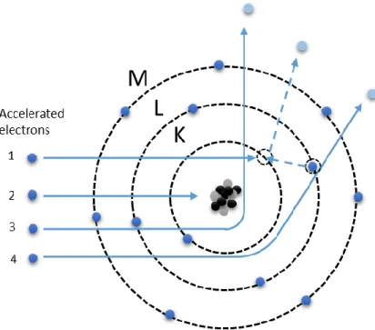
As previously mentioned in Section 2.1, W. D. Coolidge invented a new type of x-ray tube which employs the principle of the Edison effect. The Edison effect is the name given to the phenomenon observed by Edison, which was the flow of electrons to a cool metal plate in an evacuated chamber from a heated metal filament (thermionic emission). In a typical x-ray source, electrons discharged from the heated filament are accelerated towards a metal surface target by applying a voltage between the metal filament and the target metal. The accelerated electron stream collides with the target of the x-ray tube, resulting in the kinetic energy of the electrons being converted to heat, light and x-rays 2. The x-rays are produced by two processes: Bremsstrahlung radiation and characteristic radiation.
2.2.1 Bremsstrahlung X-rays
Bremsstrahlung x-rays are the primary source of x-rays from an x-ray tube 3. The accelerated stream of electrons penetrate the anode target material, approaching the strong positive nuclear field of one of its atoms. The strong attraction between the opposite charges causes the electron to deviate from its initial part2,3. The deceleration of the electron results in a loss of kinetic energy which is radiated as an x-ray of equal energy2. Accelerated electrons vary in speeds at which they approach the target metal, and how closely they approach the nuclei. As different electrons decelerate differently, the corresponding loss of kinetic energy varies,
resulting in x-rays with varying energy2. Electrons may have multiple bremsstrahlung
5
or less than the energy of the incident electron3. Figure2.1 shows the mechanism of bremsstrahlung radiation.
Figure 2.1 Illustration of four electron interactions that produce Bremsstrahlung radiation
6
Figure 2.2 An illustration of Bremsstrahlung radiation spectrum for an arbitrary peak tube voltage
2.2.2 Characteristic X-rays
Characteristic radiation is the other process by which x-rays are generated in an x-ray tube. An electron with kinetic energy E0 may interact with atoms of the anode target by ejecting an inner orbital electron (for example, K or L electron). This creates a vacancy in one of the electron orbital shells, leaving it in an ionized and excited state 2,4. Consequently, the electron hole is instantly filled by an electron from an outer valence shell. This causes energy to be given off in the form of electromagnetic radiation called characteristic radiation 2. The emitted
7
Figure 2.3 An illustration of the mechanism of characteristic x-ray production.
There are several discrete energy peaks that can arise from a number of electron
8 2.3 X-ray Interactions in matter
Most x-ray photons do not interact with atoms in the body and pass through unaffected. However, some x-ray photons undergo scattering and absorption upon interacting with a body of matter, which reduces the intensity of the ray beam. More specifically, there are four ways x-ray photons interact with atoms in their path: photoelectric absorption, Rayleigh scattering, Compton scattering, and pair production. The latter of the four is irrelevant to diagnostic radiology3.
2.3.1 Photoelectric Absorption
Photoelectric absorption occurs when an incident x-ray photon gives up all its energy to an inner orbital electron (usually K or L shell). For this to occur, the photon has to have slightly greater energy than the binding energy of an inner orbital electron. Consequent to the interaction, the electron is then emitted from the atom with kinetic energy equal to that of the photon, minus the binding energy of the electron shell, resulting in a photoelectron. The energy of a
photoelectron is expressed in the following equation:
E kinetic = hf photon – E binding (2. 1) where E kinetic is the kinetic energy of the photoelectron, hf photon is the energy of the incident photon, and E binding is the binding energy of the orbital electron3,5.
9
cascading sequence until the atom returns to its normal or ground state. The sum of energies of the characteristic photons in a single photoelectric interaction equals the binding energy of the shell from which the electron was initially expelled. In some instances, a competing process that is dominant in low atomic number elements takes place, known as Auger electron emission. This occurs when the energy released from the cascading electron is absorbed by an electron typically in the same orbital, ejecting the electron. The Auger electron’s energy is the difference between the transition energy and the binding energy of the ejected electron5.
Figure 2.4 Illustration of photoelectric absorption interaction in matter.
10
significantly important in radiography, as the photoelectric occurrence between tissue, bone and contrast enhanced agents contribute to radiographic contrast5.
2.3.2 Rayleigh Scattering
The Rayleigh scattering mechanism involves the elastic or coherent scattering of x-rays by atomic electrons. Low energy x-ray photons may interact with closely bound orbital
electrons’ electronic fields and are scattered as a result. The x-ray photon is scattered in a forward direction without any change in energy to the incident photon. The probability of
Rayleigh scattering is proportional to Z2/E, and decreases as the photon energy is increased. This scattering occurs with low energy photons well below the range required for clinical radiology. 2.3.3 Compton Scattering
Compton scattering is the inelastic scattering of x-ray photons by an outer orbital
electron. When an incident photon of adequate energy interacts with the loosely bound electron, it can displace the electron deflecting the x-ray photon in another direction (scatter photon). The resultant characteristic radiation is negligible in radiology as its energy is extremely low. This phenomenon is known as the Compton Effect and is expressed as:
𝐸𝑆𝐶 = 𝐸0
1+ 𝐸0
511 𝑘𝑒𝑉(1−𝑐𝑜𝑠𝜃)
(2. 2 ) where ESC is the energy of the scattered photon, E0 is the energy of the incident photon, and the
angle of the scattered photon5.
11
receptor, contributing scattered radiation, which is counterproductive in radiology as it contributes form of noise.
2.3.4 Pair Production
This interaction does not occur in clinical radiology as it involves photons exceeding or equal to 1.022 MeV. At this energy, photons have ample energy to overcome nuclear
electrostatic forces to be absorbed to then produce a pair of particles of equal mass: positron (positive electron) and electron.
2.4 X-ray Attenuation Tissue
The interaction mechanisms leading to the removal of photons from the x-ray beam discussed in the previous section contribute to varying degrees of attenuation in matter5. The attenuation of x-rays is what provides image contrast in medical x-ray imaging. The dominant mode of interaction of x-rays in the region on a body varies with photon energy, and the effective atomic number1. For simplification, the human body comprises of three types of body tissue: bone, muscle and fat. Also present in the body during imaging is air, present in lung cavities, and sometimes contrast enhancement agents used for the accentuation of x-rays in specific regions6. The differential absorption of tissue, air, and contrast agents results in varying intensity of photons being transmitted through the region of the body, detected by the image receptor. The amount of photons absorbed by each type of material is dependent on its linear attenuation coefficient, and thickness. If we model a polyenergetic x-ray beam as a
monoenergetic source, the amount of photon lost (n) that pass through a thin slab (Δx) of homogenous material is expressed as:
12
where is N is the number of incident photons, and µ the constant of proportionality defined as the linear attenuation coefficient3,5. The difference in the number of photons that are transmitted, to the incident photons is
∆𝑁 = 𝑁′− 𝑁 (2. 4 ) = −𝑛 (2. 5 ) = −𝜇𝑁∆ 𝑥 (2. 6 ) Since the attenuation process is a continuous quantity, the thin slab of material is treated as an infinitesimally small quantity that leads to the differential equation
𝑑𝑁
𝑁 = −𝜇 𝑑𝑥 (2. 7 )
when solved yields
𝑁 = 𝑁0𝑒−𝜇∆𝑥 (2. 8 ) where N0 is the number of incident photons, N is the number of transmitted photons, and x is the material thickness. X-ray beam intensity is proportional to the number of photons, so this
equation can be written in terms of intensity as well,
𝐼 = 𝐼0𝑒−𝜇∆𝑥 (2. 9 ) where I0 is the incident beam intensity, and I is the intensity after passing through the material.
In reality, the x-ray beam is polyenergetic having a spectrum distribution S0(E). Also, the linear attenuation coefficient depends on the composition of the material, and the spectrum distribution. Therefore the linear attenuation coefficient, µ(E), should be treated as a function of energy. Taking this into consideration the overall intensity of an x-ray beam is given by
𝐼(𝑥) = ∫ 𝑆0(𝐸′)𝐸′𝑒∫ −𝜇(𝑥
′;𝐸′)𝑑𝑥′ 𝑥
0
∞
13
This equation presents a good model for heterogeneous materials, however since µ is acutely mathematically complex, it is usually estimated and the effective energy of the polyenergetic source is used.
2.5 Conventional X-ray Tubes
The most conducive way to controllably generate x-rays is using an x-ray tube. The fundamental design of current x-ray tubes is similar to the Coolidge tube which generated x-rays thermionically. The x-ray tube consist of a cathode and anode assembly, in a glass tube housing that has been evacuated to high vacuum. The cathode is essentially a tungsten filament that emits electrons via thermionic emission. The anode consist of a metal target, and when high voltage is applied between the anode and cathode, electrons are accelerated towards the anode at high velocities. The bombardment of electrons on the target results in both Bremsstrahlung and characteristic radiation. The physics of x-ray production was previously discussed in section 2.21 and 2.22. The resulting x-ray beams emerge through the x-ray window of the tube housing. Figure 2.5 is a schematic representation of a conventional x-ray tube.
14 2.5.1 Cathode Assembly
The cathode assembly mainly consist of a filament, supporting wires and a focusing cup. In most x-ray tubes, the filament is made of coiled tungsten wire connected to supporting wires that will supply the electric current. One of these wires is also connected to a high voltage power supply, which provides the high negative potential needed to accelerate the electrons towards the anode. A low voltage (8V to 12V) is applied to the filament which generates enough current to heat the filament and energize electrons. When electrons achieve a higher energy than the work function of the metal, electrons are emitted (thermionic emission). The focusing cup is a
negatively charged concave metal cup which houses the filament. When independently supplied with a high negative voltage, it can further narrow the electron beam width to produce a small focal spot distribution on the anode.4,5
2.5.2 Anode
The anode is the origination of x-ray radiation in an x-ray tube. Since more than 99 percent of the electrons’ kinetic energy is converted to heat at the anode, the anode must be constructed of materials with high heat capacities, and it must be capable of rapid heat dissipation. In addition, anode construction requires materials of high atomic numbers for efficient of x-ray production. The most common anode target material is tungsten as it has an atomic number of 74, and a melting point of 3370oC making it suitable as a target metal 4.
15
consist of a tungsten disk, with a precisely beveled edge of the required anode angle. The anode disk inside the x-ray tube housing is connected to a metal rod arranged around bearings so that the anode can rotate freely 3. The metal rod is then connected to the rotors of an induction motor outside of the housing as seen in Figure 2.5. Throughout rotation of the anode, the electron beam bombards a “new spot” so that the heating effect spreads around a large area known as the focal track, located on the beveled face 2. An anode’s ability to accumulate, store, and discharge heat limits the power of an x-ray tube. Generally, an increase in the area of the focal track and higher anode rotation rpms allow for better heat dissipation 2,3.
2.5.3 Tube Housing
The cathode assembly and anode are enclosed in a tube usually made of a boro-silicate glass. As mentioned earlier, a high vacuum must be achieved and maintained for the generation of electron beams. As a result, the x-ray tube housing must be capable of withstanding
atmospheric pressure while under high vacuum, able to withstand heat generated by the anode, and transparent to the heat radiated from the anode. An x-ray window situated on the tube where the x-rays are directed, which is usually made of thinner material.
2.5.4 Focal Spot
16
between the requirements of a small focal spot size that produces enough photon flux coupled with prevention of melting the anode. To compensate for heat loading, the electrons are focused on a large area that is tilted relative to the incident beam causing the effective focal spot to be smaller. This is illustrated in Figure 2.6. The size of the effective focal spot is determined by the line of focus principle, giving the length of the effective focal spot size being equal to the real focus spot length times sin θ 3.
Figure 2.6 An illustration of the effect of the incident focal spot size on the effective focal spot size.
2.5.5 Window and Filter
The material of the x-ray tube window is important as it provides inherent beam
filtration. Lower energy spectrum photons play no role in the image formation, and are absorbed by the first few centimeters of tissue contributing to patient dose. The x-ray tube window serves as the initial filter, absorbing low energy photons and improving beam quality. X-ray tube windows are usually thin and made with either glass, beryllium, or aluminum.
17
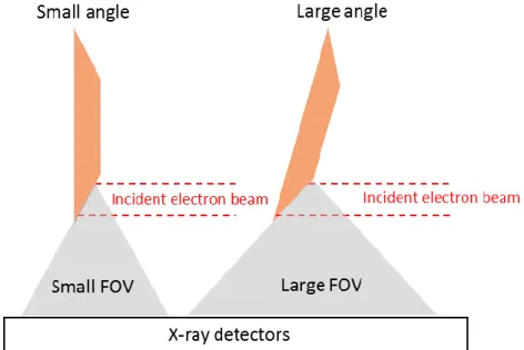
lower-energy photons. Removal of lower-energy photon increases the average energy of the spectrum, therefore giving it greater penetrating power. This is known as beam hardening. 2.5.6 Heel Effect
The Heel Effect gives rise to the non-uniformity of photon intensity across an x-ray beam. It is affected by the anode angle; an increase in anode angle, decreases the heel effect. This effect occurs when x-rays emitted near the anode are attenuated by the anode, reducing the x-ray flux to the image receptor. Consequently, the intensity of an x-ray beam decreases in the direction of the cathode to the anode. This effect is noticeable in clinical radiology as diagnostic tubes use low x-ray energies with steep anode angles. X-ray beams are usually collimated, or using a compensating filter to improve beam uniformity.
18
2.6 REFERENCES
1 W.R. Hendee and E.R. Ritenour, Medical Imaging Physics (Wiley-Liss, 2002).
2 J. Selman, The Fundamentals of Imaging Physics and Radiobiology, Ninth (Charles C Thomas, Springfield, Illinnois, 2000).
3 J.L. Prince and J.M. Links, Medical Imaging Signals and Systems (Pearson Prentice Hall, Upper Saddle River, New Jersey, 2006).
4 F.M. Khan, The Physics of Radiation Therapy (Lippincott Williams & Wilkins, 2010).
5 J.T. Bushberg, J.A. Seibert, E.M. Leidholdt, J.M. Boone, and M. Mahesh, Med. Phys. 40, 077301 (2013).
19
CHAPTER 3:Fundamentals of Mammographic Imaging 3.1 Breast Cancer Screening
Screening is a method whereby swift postulation of an unsuspected disease can be determined by means of an examination or other procedure in a population of asymptomatic women. The qualities of an ideal screening test include having high detection rates of cancers (true positive), and low false detection rates (false-positive), that subject patients to further unnecessary diagnostic testing1–3. Essentially, a screening test should result in earlier detection of disease than previous methods, and ultimately result in the reduction of mortalities from the disease, or a major benefit such as eliminating the need for dangerous, harsh, or more invasive methods. Additionally, the degree of benefit must outweigh associated human risks, and economical aspect of the screening method 3,4.
Cancer screening procedures are developed by regulatory bodies in individual countries based on the national cancer incident and occurrence within the population. Specifics such as, age and frequency of screening coupled with cost must be taken into consideration. In addition, quality control measures must be implemented to ensure accuracy, consistency, and overall efficacy for screening equipment.
20 3.2 X-ray Mammography
Mammographic imaging is a medical imaging technique that uses low dose x-rays to obtain images of the breast anatomy. Specific equipment and techniques have been developed for the optimization of breast imaging since breasts are solely made up of soft tissue that have
similar radiographic properties1,5,6. For breast cancer screening, effectiveness is measured through clinical studies. Mammography has been shown to be significantly effective in the reduction of breast cancer mortality in randomized clinical trials as well as systematized screening studies5. X-ray mammography is the only noninvasive way for early detection of breast cancer in asymptotic patients.
The aim of x-ray mammography is to produce images with high spatial resolution that show the internal structure of the breast. Fine detail of the internal structure is necessary to detect mammographic features that are characteristic of breast cancer3. To further understand the requirements for x-ray mammography, the breast anatomy, and breast cancer features are covered in this chapter prior to description of mammographic imaging systems.
3.2.1 Breast Anatomy and mammographic features of breast cancer
The breast anatomy consist of adipose, glandular, and connective tissue. The tissue overlays the pectoral muscle extending from the clavicle down to the mid-sternum, and from the lateral border of the sternum to the axilla. The glandular tissue consist of lobules connected to the nipple by ducts (Figure 3.1), which are responsible for the lactation in breast. The darker skinned region around the nipple is called the areola. Fatty tissue surrounds the glands
21
Figure 3.8 Diagram of breast anatomy. The diagram shows the major and surrounding structures of the breast. Image adapted from original © Patrick J Lynch. Reprinted with permission from the copyrighter based on the Creative Commons Attribution from Wikipedia.com
An important feature in the mammogram is determining the amount of glandular tissue present in the breast. On an x-ray image, the glandular tissue which is denser looks mostly white, while the adipose tissue looks like dark shades of grey. The ratio of the tissue on the
22
Table 3. 1 ACR BI-RADS Terms for Breast Density. Adapted from ACR BI-RADS Atlas 5th Edition8,9.
Classification Description Percentage Glandular
Tissue
a Mostly Fat < 25%
b Scattered Fibroglandular 25 – 50 %
c Heterogeneously Dense 51 – 75 %
d Extremely Dense >75%
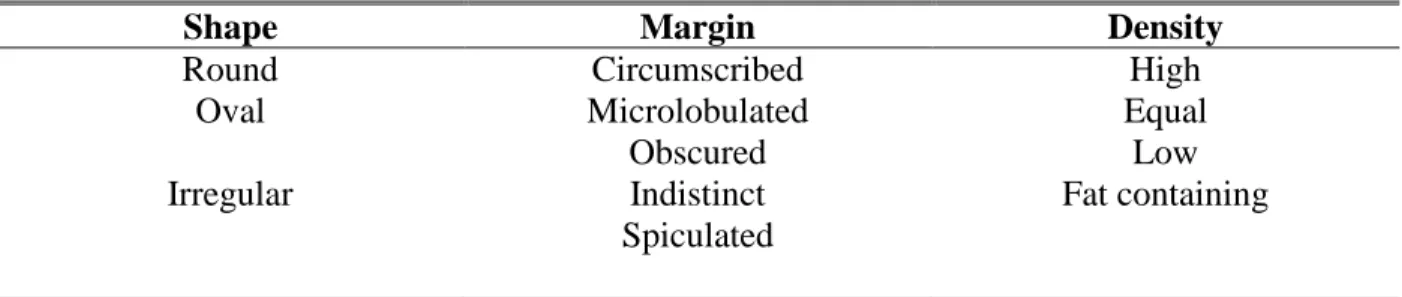
The two general categories of mammographic findings that are indicative of cancer are masses and clustered microcalcifications. According to the ACR BI-RADS terminology, a breast mass is defined as a three-dimensional space occupying lesion that is seen on two
mammographic projections2. With a few exceptions, benign masses (non-cancerous) do not penetrate surrounding tissue, and have rounding (well delineated) borders, whereas malignant tissue extends through the basement membrane, invading surrounding glandular tissue. As a result, malignant masses are irregularly shaped with indistinct or spiculated margins. As the mass shape becomes more irregular, or mass margins become more spiculated, the probability that it is a cancer increases. Mass density is also important in determining whether the mass is malignant or benign. Its density is determined with respect to the fibroglandular tissue in the patient breast. Higher density masses have a higher chance of being cancers, though low-density ones do exist. Table 3.2 is a description of malignant masses according to ACR BI-RADS lexicon.
Table 3. 2 Description of the types of malignant masses according to ACR BR-RADS lexicon. Adapted from ACR BI-RADS Atlas 5th Edition8,9
Shape Margin Density
Round Circumscribed High
Oval Microlobulated Equal
Obscured Low
Irregular Indistinct Fat containing
23
Associated calcifications in and around suspicious masses are also of concern since it may represent cancer. Calcifications are also present without masses which need to be analyzed as it may be the only indication of cancer. The prevalence of microcalcifications in
mammograms are high, yet most microcalcifications are benign. Therefore, it is important to recognize individual size, and morphology and location of the cluster to determine whether cancer is present2. Calcifications are usually found within the ducts of the breast and
consequently take on the shape of the duct. The ACR BIRADS nomenclature for the assessment of microcalcifications are displayed in Table 3.3.
Table 3.3 . Description of the types of calcification clusters according to ACR BR-RADS lexicon Adapted from ACR BI-RADS Atlas 5th Edition8,9
Calcification
Typically benign Suspicious morphology Distribution
Skin Amorphous Diffuse
Vascular Coarse heterogeneous Regional
Coarse or “popcorn-like” Fine pleomorphic Grouped
Large rod-like Fine linear or fine-linear branching Linear
Round Segmental
Rim Dystrophic
Milk of calcium Suture
3.3 X-ray Mammographic Imaging
24
important, as their size, morphology, and distribution are instrumental in diagnosis of diseased tissue3,4. For the reason that x-ray mammography systems have to enhance the contrast between tissues of small attenuation differences, and detect microcalcifications while keeping patient dose to a minimum, dedicated x-ray tubes and other equipment are essential for x-ray mammography imaging1,3. In order to ensure that optimal images are produced at the lowest possible patient dosage, quality control procedures have to be adhered to, which govern the design, and operation of an x-ray mammography system1. This is further discussed in the following sections.
3.3.1 Influences on imaging quality
There are two factors that contribute to mammographic image quality: technical and clinical factors. Assuming that there is a close correlation between the two, only the technical aspects would be considered in this section. Mammographic image quality is the measure of how well the image achieves its purpose in demonstrating whether disease is present or not in the breast. The image must distinctly display physiological, and anatomical structures, including deviations from normal tissue caused by disease or injury10. A high quality mammogram should be able to depict features such as asymmetry between the left and right breast, distortions of normal structure of the breast tissue, characteristic morphology of masses, and the shape and distribution of calcifications1,3. Several factors affect the extent to which these features are rendered optimal, and are the focus of this section.
Spatial Resolution
25
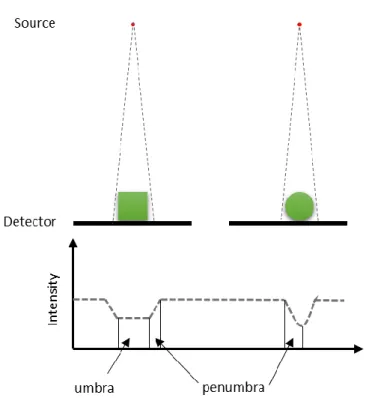
unsharpness. The degree to which blurring increases, increases with the focal spot size, therefore a smaller focal spot size is favorable. Figure 3.2(b) illustrates the relationship with the source to object and source to detector distance relationship in geometric unsharpness. For a given size source, the extent of unsharpness decreases with an increase in the source to object distance. This can be done in either one of two ways, by moving the source further away from the object, or by moving the object closer to the image receptor3,10. Geometric unsharpness becomes particularly important in spot magnification mammography. The ratio of the source to object distance (SOD) to source to imager distance (SID) governs the magnification at which the region of interest is imaged. For magnified imaging, the ratio of the SOD to SID is increased by raising the breast closer to the source. Accordingly, the geometric unsharpness is increased and is compensated for by using a focal spot of smaller size3.
Figure 3.9 (Left) Schematic diagram showing the effect of focal spot size on resolution. (Right) Schematic diagram illustrating x-ray magnification
26
Subject unsharpness is sometimes referred to as absorption unsharpness. It can be the result of the composition of the object’s structure in the patient, the shape of the object, or a combination of both10. This sometimes leads to a structure being anatomically indistinguishable from its background. Figure 3.3 shows a schematic diagram of the unsharpness due to the shape of an object.
Figure 3.10 Illustration showing unsharpness in x-ray profile due to the shape of the object.
27
The image receptor is responsible for the formation of the final image, and the detector specifications dictate imaging parameters in mammography3. There is inherent unsharpness regardless of the type of image receptor used. In screen film mammography, thickness and composition of the light sensitive emulsion on the screen film influences the sharpness of structures in an image. Unsharpness increases with increasing thickness of the light sensitive emulsion, but the thicker the layer, the more sensitive it is to light1. Therefore, a compromise has to be made with the composition of the film and thickness to optimize sensitivity and sharpness in short imaging times. In digital mammography, the digital receptors and display affect image sharpness. Data can be received and displayed in different modes that affect the level of
unsharpness. Generally, digital receptors with smaller pixel sizes generate sharper images.
Contrast
Contrast is another key contributor to image quality in mammographic imaging. It indicates the degree to which subtle anatomical and physiological structures in the region of interest are differentiable in the image. The difference in radiolucency of the tissue being imaged, imaging receptor, and display methods are key contributing factors10.
28
homogenous x-ray beam of incidence passing through the tissue of uniform attenuation coefficient, µ and varying thickness and composition, the intensity of the photons exiting the different regions will be different. The contrast is calculated as a difference in the signals, for example, the contrast between region 1 and region 3 is given by:
𝐶𝑆 = 𝐼𝐵− 𝐼𝑂
𝐼𝐵 (3. 11 )
where CS is the subject contrast, IB intensity of the background, and IO intensity in the region of the object. The intensity of photons exiting an object after traversing through an object is dependent on the attenuation coefficient and thickness. Synonymous to increasing thickness, increasing the attenuation coefficient, µ, decreases the signal1. Since the breast is made up of soft tissue, lower energies with higher attenuation coefficient, and larger differential in attenuation values in the tissue are used to increase contrast between them.
29
The imaging receptor converts the photons into intensity signals, and its characteristics are instrumental in producing contrast of the final image. Its contrast is determined by how well it can convert the differences in energy leaving the object into an output intensity signal1,10. Specific to digital mammography, the contrast in the display can also be changed, within a dynamic range of the digital monitor.
Noise
Image noise is the information in an image that is useless, and a contributor to image degradation in x-ray imaging. All radiologic systems have some amount of noise. Sources of noise are from the tissue structure, radiation, the receptor, and quantum noise1,10. Structure noise arises from the shadows of structures in the tissue that do not contribute information to the image. It is frequently responsible for missed lesions and abnormalities in images. Because of the breast volume and structure, it is standard for two projection views of each breast to be obtained for either screening or diagnostic imaging. The two views allow for an understanding of the superimposed structures that are present if only one view is taken, a means of working around structure noise.
non-30
uniformity in the image, and reducing the definition of structures3,11. Sources that allow for sufficient photon flux, or longer exposures are necessary for the reduction of quantum noise.
Signal Difference-to-Noise Radio
Since noise is counterproductive to visualization of objects in radiographic images, contrary to contrast and spatial resolution, it is useful to use the signal difference-to-noise ratio (SDNR) for the characterization of image quality5. The SDNR is the ratio of the detected signal difference to the standard deviation,
𝑆𝐷𝑁𝑅 =𝑆𝑅𝑂𝐼− 𝑆𝐵
𝜎𝐵 (3. 12 )
Where SROI is the average signal for the ROI, SB the average signal of the background, and 𝜎𝐵 the standard deviation of the background. It is more meaningful to consider a region than to consider evaluating single pixels as it corresponds to a lesion or object of interest, to an equal area of the nearby background5.
3.3.2 Mammographic equipment
Each component of an x-ray mammography system influences the quality of the resulting image. Understanding the composition of normal, and diseased breast tissue, and influences on mammographic imaging have led to the development of specific techniques, x-ray tube and system designs. In addition, the risks associated with ionizing radiation requires minimizing dose while keeping images optimal.
The x-ray tube design is the single most important component of a dedicated
31
larger of the focal spots usually has a nominal size of 0.3mm, while the smaller has a size of 0.1 mm1. The larger focal spot is used in standard mammography imaging where views of the entire breast are needed. When specific areas of the breast need to imaged, for example
microcalcification clusters, magnified views are needed. The use of the smaller focal spot minimizes geometric blurring and maintain the spatial resolution necessary for visualization of microcalcifications1. Rotation anodes are employed as a means to maximize tube amperage and minimize imaging time. The anode placement away from the chest wall (nipple side), and cathode placement over the chest wall achieves a more even distribution of transmitted x-ray as the heel effect is further away from the patient. An effective anode angle of ~22o relative to the plane of the detector, for a source to detector distance of 65 cm is typical for total detector coverage. The x-ray tube must be capable of producing an acceptable tube output as defined by MQSA.
32
Other essential equipment necessary for mammography includes collimators,
compression paddles, and anti-scatter grids. Collimators are fixed size metal apertures used to define the radiation field, focusing x-rays in the region of interest, and reducing scatter.
Compression paddles are employed to reduce movement and achieve uniform tissue thickness. This yields less motion blur, and geometric blur of structures, as they are closer to the detector. It also acts to further reduce the amount of tissue overlap resent in 2D mammography1.
Mammography systems also use antiscatter grids placed between the breast and the image receptor to reduce the scattered radiation transmitted through the breast.
Image receptors are another critical component of x-ray mammography machines. They are needed to provide imaging contrast, sufficient spatial resolution, and to allow for fast imaging times. There are currently two types of x-ray mammography machines: screen-film mammography and full field digital mammography. Screen film mammography involves using a cassette containing a screen film that needs to be developed as the image receptor. In full field digital mammography, the imaging receptor converts the photons into digital information, which is then sent to a digital monitor to be viewed. Both types of image receptors have particular requirements, and dictate the imaging parameters of the system3. These are discussed in the following two sections.
3.4 Mammographic modalities 3.4.1 Screen Film Mammography
Screen film mammography systems utilize film as the detector and the display medium. This introduces inherent disadvantages since imaging parameters have to be optimized to satisfy both imaging and viewing parameters, making all parameters interrelated. As a result,
33
The mammography system’s x-ray tube and geometry governs imaging parameters, making it critically important in determining the rate of exposure and beam quality of the x-ray beam. The x-ray tube, together with its power, distance, and the screen/film detector efficiency influences the time needed to produce an optimal image. This introduces a tradeoff between resolution and imaging speed. Ultimately, the overall system resolution is limited by the screen film detector’s capacity to record and display the details of the breast that the other components of the system present 3.
34
Figure 3.13 Schematic diagram of a screen film detector.
An additional limitation of film is that once the image is developed, it is unchangeable. Therefore, if the processed image is not optimal, it may result in repetition that introduces greater dose to the patient. It is also the only record of the image; therefore if it is misplaced, it cannot be retrieved. The physical space needed for the storage of x-rays images is another disadvantage. 3.4.2 Full Field Digital Mammography
The advent of digital detectors brought about the development of the digital
mammography system. Digital mammography, contrary to SFM separates the acquisition of the image and its corresponding image display. Consequently, each part of the imaging sequence can be optimized giving this system unique properties. Mammography presents a great challenge for digital detectors because of the high spatial resolution required.
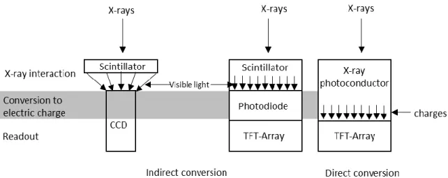
There are two main types of digital detectors used in mammography are indirect and direct detectors. Indirect detectors use a process that is synonymous to SFM, it uses a scintillator (usually cesium iodine) to absorb x-rays and generate a light scintillation. The scintillators are paired with either charged-coupled devices or thin-film transistor (TFT) panels. The CCD
35
by pixel, then digitized and stored on a computer system12. For indirect detectors using TFT panels, the converted light first encounters a photodiode layer that converts the visible light into electric charges. The TFT readout circuitry then transforms the charges into digital values for an image to be displayed and stored 12. Both indirect systems have an intrinsic degradation of resolution due to the scintillator screen spreading light.
Direct conversion detectors consist of an x-ray photoconducting layer that is grown directly onto a TFT charge collector and readout layer. Amorphous selenium is typically used as the photoconducting layer due to its superb x-ray detection properties, and high spatial resolution 12. Prior to ray exposure, an electric field is applied across the a-Se layer. During exposure, x-ray photons incident upon the layer of a-Se generates electrons and holes, and these charges migrate perpendicularly to the a-Se layer to the electrodes below without much lateral diffusion. The charges are stored in the charge-collection electrodes until readout3,12.
Because of the conversion of analog signals to a digital matrix of number, compromises are made on the spatial resolution. For example, film screens have spatial resolutions greater than 20 cycles/mm, which would require a digital detector with pixel sizes of 25 µm. Very specialized monitors, and hard drives with huge capacities would have to be employed to realize this
36
Figure 3.14 Illustration of the two types of digital detectors, indirect and direct conversion.
Advantages of digital mammography systems include the ability to post process. Over or under exposed mammograms can be corrected as image processing and image acquisition are separated. Image handling and storage is also made easier as it can be accessible on any computer with the appropriate equipment, and each mammogram does not require its own physical space.
3.4.3 Contrast Enhanced Full Field Digital mammography
Full field digital mammography developments have been rapid, leading to the
development of other advanced imaging techniques5. Though the diagnostic accuracy of FFDM is at least equivalent to screen-film mammography5, there are still some limitations. Particularly in dense breast, and patients with fibrocystic disease, cancers are difficult to detect. The
37
that are metabolically active. The difference in x-ray attenuation of the two regions are exploited to effectively cancel background tissue, leaving only the iodinated region.
In temporal subtraction, a radiographic image of the breast is taken prior to the injection of the iodinated contrast agent then another at the same x-ray tube energy. The presence of iodine in the post contrast image would increase contrast of the region, while attenuation of the normal tissue will remain the same as the pre-contrast image. In order to enhance the iodinated region, the pre-contrast image is subtracted from the post-contrast image. To avoid image artifacts and attain optimum image quality, the best image registration is required. As a result, imaging must be quick, using light breast compression that will allow for blood flow, while restricting motion between the pre-contrast and post-contrast image.