Exploring cosmic origins with CORE: Mitigation of systematic effects

July 14, 2017 Prepared for submission toJCAP

Exploring cosmic origins with CORE:

mitigation of systematic effects

P. Natoli,

1,2,a

M. Ashdown,

3,4

R. Banerji,

5

J. Borrill,

6,7

A. Buzzelli,

8,9,10

G. de Gasperis,

9,10

J. Delabrouille,

5

E. Hivon,

11

D. Molinari,

1,2,12

G. Patanchon,

5

L. Polastri,

1,2

M. Tomasi,

13,14

F. R. Bouchet,

11

S. Henrot-Versill ´e,

15

D. T. Hoang,

5

R. Keskitalo,

6,7

K. Kiiveri,

16,17

T. Kisner,

6

V. Lindholm,

16,17

D. McCarthy,

18

F. Piacentini,

8,19

O. Perdereau,

15

G. Polenta,

20,21

M. Tristram,

15

A. Achucarro,

22,23

P. Ade,

24

R. Allison,

25

C. Baccigalupi,

26,27

M. Ballardini,

12,28,29

A. J. Banday,

30,31

J. Bartlett,

5

N. Bartolo,

32,33,34

S. Basak,

35,26

J. Baselmans,

36,37

D. Baumann,

38

M. Bersanelli,

13,14

A. Bonaldi,

39

M. Bonato,

40,26

F. Boulanger,

41

T. Brinckmann,

42

M. Bucher,

5

C. Burigana,

12,1,29

Z.-Y. Cai,

43

M. Calvo,

44

C.-S. Carvalho,

45

G. Castellano,

46

A. Challinor,

38

J. Chluba,

39

S. Clesse,

42

I. Colantoni,

46

A. Coppolecchia,

8,19

M. Crook,

47

G. D’Alessandro,

8,19

P. de Bernardis,

8,19

G. De Zotti,

34

E. Di Valentino,

11,48

J.-M. Diego,

49

J. Errard,

50

S. Feeney,

3,51

R. Fernandez-Cobos,

49

F. Finelli,

12,29

F. Forastieri,

1,2

S. Galli,

11

R. Genova-Santos,

52,53

M. Gerbino,

54,55

J. Gonz ´alez-Nuevo,

56

S. Grandis,

57,58

J. Greenslade,

3

A. Gruppuso,

12,29,1

S. Hagstotz,

57,58

S. Hanany,

59

W. Handley,

3,4

C. Hernandez-Monteagudo,

60

C. Herv´ıas-Caimapo,

39

M. Hills,

47

E. Keih ¨anen,

16,17

T. Kitching,

61

M. Kunz,

62

H. Kurki-Suonio,

16,17

L. Lamagna,

8,19

A. Lasenby,

3,4

M. Lattanzi,

2,1

J. Lesgourgues,

42

A. Lewis,

63

M. Liguori,

32,33,34

M. L ´

opez-Caniego,

64

G. Luzzi,

8

B. Maffei,

41

N. Mandolesi,

1,12

E. Martinez-Gonz ´alez,

49

C.J.A.P. Martins,

65

S. Masi,

8,19

A. Melchiorri,

8,19

J.-B. Melin,

66

M. Migliaccio

20,9

A. Monfardini,

44

M. Negrello,

24

A. Notari,

67

L. Pagano,

41

A. Paiella,

9,19

D. Paoletti,

12

M. Piat,

5

G. Pisano,

24

A. Pollo,

68

V. Poulin,

42,69

M. Quartin,

70,71

M. Remazeilles,

39

M. Roman,

72

G. Rossi,

73

J.-A. Rubino-Martin,

52,53

L. Salvati,

9,19

G. Signorelli,

74

A. Tartari,

5

D. Tramonte,

52

N. Trappe,

18

T. Trombetti,

12,1,29

C. Tucker,

24

J. Valiviita,

16,17

R. Van de Weijgaert,

75,76

B. van Tent,

77

V. Vennin,

78

P. Vielva,

49

N. Vittorio,

9,10

C. Wallis,

39

K. Young,

59

and M. Zannoni

79,80

for the CORE collaboration.

a_{Corresponding author}

1_{Dipartimento di Fisica e Scienze della Terra, Universit`a di Ferrara, Via Saragat 1, 44122 Ferrara,}

Italy

2_{INFN, Sezione di Ferrara, Via Saragat 1, 44122 Ferrara, Italy}

3_{Astrophysics Group, Cavendish Laboratory, University of Cambridge, J. J. Thomson Avenue,}

Cam-bridge, CB3 0HE, UK

4_{Kavli Institute for Cosmology, Univerisity of Cambridge, Madingley Road, Cambridge, CB3 0HA,}

UK

5_{APC, AstroParticule et Cosmologie, Universit´e Paris Diderot, CNRS/IN2P3, CEA/lrfu,}

Observa-toire de Paris, Sorbonne Paris Cit´e, 10, rue Alice Domon et L´eonie Duquet, 75205 Paris Cedex 13, France

6_{Computational Cosmology Center, Lawrence Berkeley National Laboratory, Berkeley, California,}

U.S.A.

7_{Space Sciences Laboratory, University of California, Berkeley, CA, 94720, USA}

8_{Dipartimento di Fisica, Universit`a di Roma La Sapienza , P.le A. Moro 2, 00185 Roma, Italy</sub> 9<sub>Dipartimento di Fisica, Universit`a di Roma Tor Vergata, Via della Ricerca Scientifica 1, I-00133,}

Roma, Italy

10_{INFN, Sezione di Tor Vergata, Via della Ricerca Scientifica 1, I-00133, Roma, Italy}

11_{Institut d’ Astrophysique de Paris (UMR7095: CNRS & UPMC-Sorbonne Universities), F-75014,}

Paris, France

12_{INAF/IASF Bologna, via Gobetti 101, I-40129 Bologna, Italy}

13_{Dipartimento di Fisica, Universit`a degli Studi di Milano, Via Celoria, 16, Milano, Italy} 14_{INAF/IASF Milano, Via E. Bassini 15, Milano, Italy}

15_{Laboratoire de l’Acc´el´erateur Lin´eaire, Univ. Paris-Sud, CNRS/IN2P3, Universit´e Paris-Saclay,}

Orsay, France

16_{Department of Physics, Gustaf H¨allstr¨omin katu 2a, University of Helsinki, Helsinki, Finland} 17_{Helsinki Institute of Physics, Gustaf H¨allstr¨omin katu 2, University of Helsinki, Helsinki, Finland} 18_{Department of Experimental Physics, Maynooth University, Maynooth, Co. Kildare, W23 F2H6,}

Ireland

19_{INFN, Sezione di Roma, P.le Aldo Moro 5, I-00185, Roma, Italy}

20_{Agenzia Spaziale Italiana Science Data Center, Via del Politecnico snc, 00133, Roma, Italy} 21_{INAF - Osservatorio Astronomico di Roma, via di Frascati 33, Monte Porzio Catone, Italy} 22_{Instituut-Lorentz for Theoretical Physics, Universiteit Leiden, 2333 CA, Leiden, The Netherlands} 23_{Department of Theoretical Physics, University of the Basque Country UPV/EHU, 48040 Bilbao,}

Spain

24_{School of Physics and Astronomy, CardiffUniversity, The Parade, CardiffCF24 3AA, UK} 25_{Institute of Astronomy, University of Cambridge, Madingley Road, Cambridge, CB3 0HA, UK} 26_{SISSA, Via Bonomea 265, 34136, Trieste, Italy}

27_{INFN, Sezione di Trieste, Via Valerio 2, I - 34127 Trieste, Italy}

28_{DIFA, Dipartimento di Fisica e Astronomia, Universit´a di Bologna, Viale Berti Pichat, 6/2, I-40127}

Bologna, Italy

29_{INFN, Sezione di Bologna, Via Irnerio 46, I-40127 Bologna, Italy}

32_{Dipartimento di Fisica e Astronomia ‘Galileo Galilei’, Universit`a degli Studi di Padova, Via}

Mar-zolo 8, I-35131, Padova, Italy

33_{INFN, Sezione di Padova, Via Marzolo 8, I-35131 Padova, Italy}

34_{INAF-Osservatorio Astronomico di Padova, Vicolo dell’Osservatorio 5, I-35122 Padova, Italy} 35_{Department of Physics, Amrita School of Arts & Sciences, Amritapuri, Amrita Vishwa Vidyapeetham,}

Amrita University, Kerala 690525, India

36_{SRON (Netherlands Institute for Space Research), Sorbonnelaan 2, 3584 CA Utrecht, The}

Nether-lands

37_{Terahertz Sensing Group, Delft University of Technology, Mekelweg 1, 2628 CD Delft, The}

Nether-lands

38_{DAMTP, Centre for Mathematical Sciences, University of Cambridge, Wilberforce Road,}

Cam-bridge, CB3 0WA, UK

39_{Jodrell Bank Centre for Astrophysics, Alan Turing Building, School of Physics and Astronomy,}

The University of Manchester, Oxford Road, Manchester, M13 9PL, U.K.

40_{Department of Physics & Astronomy, Tufts University, 574 Boston Avenue, Medford, MA, USA} 41_{Institut d’Astrophysique Spatiale, CNRS, UMR 8617, Universit´e Paris-Sud 11, Bˆatiment 121,}

91405 Orsay, France

42_{Institute for Theoretical Particle Physics and Cosmology (TTK), RWTH Aachen University,}

D-52056 Aachen, Germany.

43_{CAS Key Laboratory for Research in Galaxies and Cosmology, Department of Astronomy,}

Univer-sity of Science and Technology of China, Hefei, Anhui 230026, China

44_{Institut N´eel, CNRS and Universit´e Grenoble Alpes, F-38042 Grenoble, France}

45_{Institute of Astrophysics and Space Sciences, University of Lisbon, Tapada da Ajuda, 1349-018}

Lisbon, Portugal

46_{Istituto di Fotonica e Nanotecnologie - CNR, Via Cineto Romano 42, I-00156 Roma, Italy} 47_{STFC - RAL Space - Rutherford Appleton Laboratory, OX11 0QX Harwell Oxford, UK} 48_{Sorbonne Universit´es, Institut Lagrange de Paris (ILP), F-75014, Paris, France}

49_{IFCA, Instituto de F´ısica de Cantabria (UC-CSIC), Av. de Los Castros s/n, 39005 Santander, Spain} 50_{Institut Lagrange, LPNHE, Place Jussieu 4, 75005 Paris, France.}

51_{Center for Computational Astrophysics, 160 5th Avenue, New York, NY 10010, USA} 52_{Instituto de Astrof´ısica de Canarias, C/V´ıa L´actea s/n, La Laguna, Tenerife, Spain}

53_{Departamento de Astrof´ısica, Universidad de La Laguna (ULL), La Laguna, Tenerife, 38206 Spain} 54_{The Oskar Klein Centre for Cosmoparticle Physics, Department of Physics, Stockholm University,}

AlbaNova, SE-106 91 Stockholm, Sweden

55_{The Nordic Institute for Theoretical Physics (NORDITA), Roslagstullsbacken 23, SE-106 91}

Stock-holm, Sweden

56_{Departamento de F´ısica, Universidad de Oviedo, C. Calvo Sotelo s/n, 33007 Oviedo, Spain} 57_{Faculty of Physics, Ludwig-Maximilians Universit¨at, Scheinerstrasse 1, D-81679 Munich,}

Ger-many

58_{Excellence Cluster Universe, Boltzmannstr. 2, D-85748 Garching, Germany}

59_{School of Physics and Astronomy and Minnesota Institute for Astrophysics, University of}

Min-nesota/Twin Cities, USA

60_{Centro de Estudios de F´ısica del Cosmos de Arag´on (CEFCA), Plaza San Juan, 1, planta 2,}

61_{Mullard Space Science Laboratory, University College London, Holmbury St Mary, Dorking,}

Sur-rey RH5 6NT, UK

62_{D´epartement de Physique Th´eorique and Center for Astroparticle Physics, Universit´e de Gen`eve,}

24 quai Ansermet, CH–1211 Gen`eve 4, Switzerland

63_{Department of Physics and Astronomy, University of Sussex, Falmer, Brighton, BN1 9QH, UK} 64_{European Space Agency, ESAC, Planck Science Office, Camino bajo del Castillo, s/n, Urbanizaci´on}

Villafranca del Castillo, Villanueva de la Ca˜nada, Madrid, Spain

65_{Centro de Astrof´ısica da Universidade do Porto and IA-Porto, Rua das Estrelas, 4150-762 Porto,}

Portugal

66_{CEA Saclay, DRF/Irfu/SPP, 91191 Gif-sur-Yvette Cedex, France}

67_{Departamento de F´ısica Qu`antica i Astrof´ısica i Institut de Ci`encies del Cosmos, Universitat de}

Barcelona, Mart´ıi Franqu`es 1, 08028 Barcelona, Spain

68_{National Center for Nuclear Research, ul. Ho˙za 69, 00-681 Warsaw, Poland, and The Astronomical}

Observatory of the Jagiellonian University, ul. Orla 171, 30-244 Krak´ow, Poland

69_{LAPTh, Universit´e Savoie Mont Blanc & CNRS, BP 110, F-74941 Annecy-le-Vieux Cedex, France} 70_{Instituto de F´ısica, Universidade Federal do Rio de Janeiro, 21941-972, Rio de Janeiro, Brazil} 71_{Observat´orio do Valongo, Universidade Federal do Rio de Janeiro, Ladeira Pedro Antˆonio 43,}

20080-090, Rio de Janeiro, Brazil

72_{LPNHE, CNRS-IN2P3 and Universit´es Paris 6 & 7, 4 place Jussieu F-75252 Paris, Cedex 05,}

France

73_{Department of Astronomy and Space Science, Sejong University, Seoul 143-747, Korea} 74_{INFN, Sezione di Pisa, Largo Bruno Pontecorvo 2, 56127 Pisa, Italy}

75_{SRON (Netherlands Institute for Space Research), Sorbonnelaan 2, 3584 CA Utrecht, The}

Nether-lands

76_{Terahertz Sensing Group, Delft University of Technology, Mekelweg 1, 2628 CD Delft, The}

Nether-lands

77_{Laboratoire de Physique Th´eorique (UMR 8627), CNRS, Universit´e Paris-Sud, Universit´e Paris}

Saclay, Bˆatiment 210, 91405 Orsay Cedex, France

78_{Institute of Cosmology and Gravitation, University of Portsmouth, Dennis Sciama Building,}

Burn-aby Road, Portsmouth PO1 3FX, United Kingdom

79_{Dipartimento di Fisica, Universit`a di Milano Bicocca, Milano, Italy} 80_{INFN, sezione di Milano Bicocca, Milano, Italy}

E-mail:[email protected]

Abstract.We present an analysis of the main systematic effects that could impact the measurement

to systematics, showing how COREcan achieve its calibration requirements. While a fine-grained assessment of the impact of systematics requires a level of knowledge of the system that can only be achieved in a future study phase, the analysis presented here strongly suggests that the main ar-eas of concern for the CORE mission can be addressed using existing knowledge, techniques and algorithms.

Contents

1 Introduction 1

2 Map-making for CMB experiments 3

3 Simulations 4

4 Analysis of simulated noise maps 6

4.1 Baseline scanning strategy 9

4.2 Optimizing the scanning strategy 11

4.3 1/f noise performance 13

5 Cross-correlated noise 14

6 Bandpass mismatch 16

6.1 Model of the bandpass mismatch effect 18

6.2 Simulations of the bandpass mismatch effect 19

6.3 Correction algorithm 19

7 Asymmetric beam 21

7.1 Real space convolution and first-order de-projection 23

7.2 Harmonic space 26

7.3 Beam asymmetry conclusions 27

8 Calibration 28

8.1 Time dependence of the dipole signal 30

8.2 Systematics 31

8.3 Systematics due to the Galaxy 33

9 Pointing accuracy and reconstruction uncertainty 35

10 Conclusions 36

1 Introduction

of future experiments, whose focal plane arrays will contain thousands of polarization sensitive de-tectors, will be dominated by systematics even for small scale polarization. It is therefore critical to ensure that these contaminants can be controlled to a level that does not jeopardize the science goals of the mission.

The impact of systematic effects plays a central role in the analysis of modern CMB experiments (Baxter et al. 2015;Bennett et al. 2013;BICEP2 Collaboration et al. 2016;Louis et al. 2016;Planck Collaboration et al. 2016c,f) and is the main subject of several papers as well (e.g., Griffiths and Lineweaver(2004);Karakci et al.(2013);Miller et al.(2009a);Planck Collaboration et al.(2016d)), many of them focusing specifically on polarization specific systematics and their treatment (Kaplan and Delabrouille 2002;Miller et al. 2009b;Pagano et al. 2009;Shimon et al. 2008). The definition of a systematic effect is somewhat dependent on the context. Strictly speaking, any contamination which is not the signal of interest and does not exhibit a purely stochastic behavior may be regarded as a systematic. The CMB community has traditionally used the term in a wider sense, considering any contamination that deviates from ideal, white noise as a systemetic. In this sense, long time scale (i.e., correlated or ‘1/f’) noise may be considered as a systematic contribution, while being from another point of view a purely random component with a zero expectation value.

This paper is part of a set describing the scientific performance of the proposedCOREsatellite, which is designed to map CMB polarization to an accuracy only limited by cosmic variance over a broad range of scales. It explores several aspects related to the expected quality of CORE’s polar-ization measurements. We employ a realistic simulation pipeline to produce time ordered data for a year’s worth of observations, which we then reduce to maps of intensity and polarization using a state of the art map-making code. We analyse these maps to assess the overall quality of theCORE full sky polarization measurements, in view of the proposed scanning strategy and instrumental de-sign. We include in the simulations a number of realistic effects that may impact the accuracy of the observations, and show that they are either under control or can be kept under control by employ-ing analysis techniques already used by the CMB community. The approach we follow consists in studying one effect at a time, which allows us to evaluate each contribution in isolation and carefully assess its impact. The obvious drawback is that we may miss potential interactions between different effects, a situation that may be addressed by employing full end-to-end simulations (see, e.g.,Planck Collaboration et al.(2016e)). We defer this very demanding analysis to future studies.

The plan of this paper is as follows. We provide in Sect.2a brief introduction to the CMB map-making methodology, which we use throughout this work. In Sect.3we describe the timeline-to-map simulation engine that was used in this work, based on the publicly available TOAST software pack-age. We produce noise-only maps based on a realistic noise model, which are analyzed in Sect. 4

2 Map-making for CMB experiments

This paper deals extensively with the propagation of CORE simulated data from time-ordered ob-servations (also called ‘timelines’) to maps of the sky. To provide some context, we briefly review map-making algorithms for CMB experiments. We begin by considering a simple model, which only accounts for ideal sky signal and stochastic instrumental noise, and discuss the standard approaches and their computational implications. This model will be elaborated in the following sections to include systematics contributions and to discuss specific procedures to mitigate their impact.

Map-making deals with estimation of maps from timelines containing redundant observations of the sky. This subject has closely followed experimental progress in the field. Map-making schemes devised for COBE (Lineweaver et al. 1994), whose differential measuring technique proved effective

in reducing correlated noise, were extended to maps containing millions of pixels forWMAP(Wright et al. 1996). More recent CMB experiments (includingPlanck) adopt a direct measurement scheme, as opposed to a differential one, in order to gain sensitivity and reduce the complexity of the optical system. This approach, also adopted forCORE, faces higher levels of 1/fnoise, which has to be kept under control by employing suitable analysis methods (see, e.g.,de Gasperis et al.(2005);Dor´e et al.

(2001);Natoli et al.(2001);Patanchon et al.(2008);Stompor et al.(2002);Tristram et al.(2011)) A widely employed model assumes that the timelineddepends linearly on the mapmby means of a ‘pointing’ operatorA:

d=A m+n, (2.1)

where the time-ordered vectornis a stochastic noise component with zero mean and (usually non-diagonal) covariance matrix Ntt0 ≡ hn_tn_t0i(tlabels time samples) and the vectormis a discretized image of the sky1, containing maps of the Stokes parameters for intensityI and linear polarization QandU2. The simplest possible model forAis the so-called ‘pencil beam’ approximation, which ignores the convolution of the signal by the instrumental beam. In this limit, the projection from the sky to the timeline of Eq.2.1reads:

dt =I+Qcos 2ψt+Usin 2ψt+nt, (2.2) where (I,Q,U) are the value of the Stokes parameters of the sky for a given instrumental pointing andψt is the instantaneous detector orientation with respect to a chosen celestial frame. Hence, the pencil beam pointing matrix has only three non-zero entries in each row, equal to [1,cos 2ψt,sin 2ψt]. If the instrumental beam is azimuthally symmetric, the pointing and beam convolution operations commute. If this is the case, we may retain the pencil beam approximation and look for an estimate of the beam-convolved map. On the other hand, if the beam is asymmetric the model 2.2 leads to a biased estimate of the map unless proper treatment is included. This situation is addressed in Section7below.

An estimate of the map, me, can be obtained by applying the generalized least squares (GLS)

procedure to Eq.2.1:

e

m=(ATN−1A)−1ATN−1d, (2.3) whereAT denotes the transpose of the pointing operator. The quantity (ATN−1A)−1is the covariance matrix ofme. The GLS estimate enjoys a number of desirable properties: provided the noise matrixN

1_{We shall employ the HEALPix pixelization scheme in what follows (G´orski et al. 2005).}

2_{Circular polarizationVis seldom considered for CMB, since it cannot be produced by Thomson scattering over}

is correct (in practice, it must be estimated from the data) it is the minimum variance estimator. Fur-thermore, if the noise is drawn from a multivariate Gaussian distribution, the GLS estimate becomes the maximum likelihood solution. It is, however, intractable to compute the matrix for a real world situation with trillions of time samples and millions of map pixels. The problem can be effectively solved by resorting to iterative techniques, typically employing a conjugate gradient solver (Natoli et al. 2001).

For the moment, we restrict the model to a single detector. Multiple detector maps can be trivially accounted for in the absence of noise that is correlated between detectors. If this is not the case, an optimal solution can still be obtained by taking the correlations in account. We discuss an application toCOREof this scenario is Section5below.

In the case of large datasets, it may be desirable to further reduce the computational burden. This can be achieved by using approximate versions of Eq.2.3. A straightforward way to obtain such an approximation is to model the correlated component of the noise using a set of basis functions (typically piecewise constant offsets of given constant length, although more complicated bases can be used) superimposed on white noise. The problem then reduces to finding a suitable estimate of the coefficients of the basis functions. This class of map-making codes is called destripers (see, for example, Burigana et al. 1999;Delabrouille 1998;Keih¨anen et al. 2004, 2005;Kurki-Suonio et al. 2009; Maino et al. 1999). Sophisticated implementations of these algorithms can produce results which are statistically indistinguishable from GLS map-making while requiring significantly less computational resources. In this scenario, prior information on the correlated noise properties may be needed (Kurki-Suonio et al. 2009). The most desirable feature of destriping algorithms is that they can be tuned to the desired precision while still controlling their computational cost. The latter of course scales unfavourably with precision, but in real-world applications an advantageous compromise can be usually found by tweaking the offset length. In the following we will make extensive use of a public domain implementation of a generalized destriper, MADAM (Keih¨anen et al. 2005,2010).

3 Simulations

Simulations play a number of critical roles in CMB missions:

1. Optimization of the design of the mission (both the instrument and the observation) to ensure that the dataset obtained will be sufficient to meet the science goals;

2. Validation and verification of the data analysis pipeline to ensure that the science can be ex-tracted from the mission dataset;

3. Uncertainty quantification and debiasing of the data analysis results using Monte Carlo meth-ods in lieu of the computationally intractable full data covariance matrix.

4. Encapsulation of knowledge on the data taking and processing, allowing e.g. for novel analyses outside of the team.

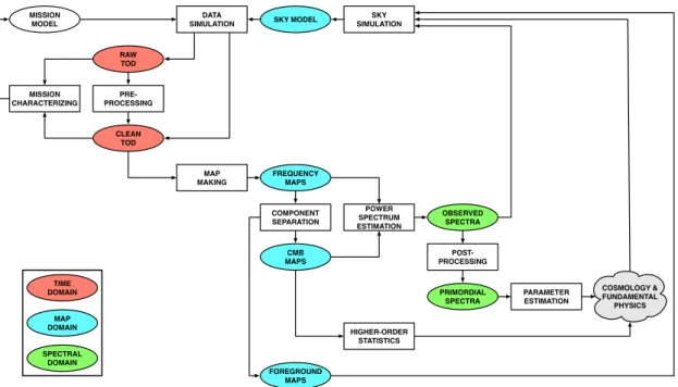
analysis pipeline alternate between mitigation of the systematic effects in the current data domain (pre-processing, component separation, post-processing) and reduction of the statistical uncertainties by transforming the data to a new domain with higher signal-to-noise (map-making, power spectrum estimation). The map- and spectral-domain products are then used to constrain the parameters of any given model of cosmology and fundamental physics, typically in conjunction with other cosmolog-ical datasets. Finally the various data representations can be used to provide feedback to refine the mission and sky models.

In this work we particularly focus on the simulation and mitigation of systematic effects to address all three questions, the optimization of the mission design, the validation and verification of the mitigation algorithms and implementations, and the quantification of the residuals after mitigation and their impact on the science results.

PRE-PROCESSING

MAP MAKING

COMPONENT SEPARATION

CMB MAPS

POWER SPECTRUM ESTIMATION

OBSERVED SPECTRA CLEAN

TOD

FREQUENCY MAPS RAW

TOD

POST-PROCESSING

PRIMORDIAL SPECTRA

COSMOLOGY & FUNDAMENTAL PHYSICS PARAMETER

ESTIMATION

HIGHER-ORDER STATISTICS DATA

SIMULATION SKY MODEL MISSION

MODEL

SKY SIMULATION

MISSION CHARACTERIZING

FOREGROUND MAPS TIME

DOMAIN

MAP DOMAIN

SPECTRAL DOMAIN

Figure 1. A schematic CMB simulation and analysis pipeline, with rectangular operators acting on oval data objects, which may be time samples (red), map pixels (blue) or spectral multipoles (green). Note the many loops, implying iterative processing.

In the absence of the explicit data covariance matrix, the most computationally challenging ele-ments of this pipeline are those that manipulate the full time-domain data, and in particular the gener-ation and analysis of Monte Carlo realizgener-ations used in lieu of this matrix for uncertainty quantificgener-ation and debiasing. Given the volume of data to be processed, we require highly optimized massively par-allel implementations of the simulation, pre-processing and map-making algorithms and significant high performance computing resources. Moreover, since data movement – whether between disk and memory or across distributed memory – is expensive, these steps must be tightly-coupled within an overall time-domain data framework. One such framework, developed for the Plancksatellite mis-sion (Planck Collaboration et al. 2016e) but with broad applicability for both satellite and suborbital CMB missions, is the Time-Ordered Astrophysics Scalable Tools (TOAST) package3_.

As well as being highly computationally efficient, any such framework must also be readily adaptable, allowing the rapid prototyping of new algorithms. TOAST is therefore implemented as a python wrapper and data management layer into which new modules can easily be dropped, cou-pled with compiled libraries (both internal and external) which can be called wherever computational efficiency is a limiting factor. TOAST has been extensively validated and verfied, primarily in con-junction with its use in thePlanckfull focal plane simulations (Planck Collaboration et al. 2016e) but also through simulations of theCOREandLiteBIRDsatellite missions, and in stand-alone compar-isons with both analytic calculations and other computational tools.

In this work the TOAST framework calls four main libraries, two internal and two external to the TOAST package:

1. the TOAST pointing library, which generates the dense-sampled pointings for each detector from the sparse-sampled satellite boresight pointing.

2. the TOAST noise simulation library, which generates timelines of noise from each detector’s piecewise stationary noise power spectral density functions, provided either as a set of arrays of explicit frequency/power pairs, or as the parameters of an analytic function (typically a white noise level and correlated noise knee frequency and spectral index).

3. the libCONVIQT beam convolution library4, a TOAST-compatible implementation of the CON-VIQT beam convolution algorithm (Pr´ezeau and Reinecke 2010), which generates timelines of sky signals from each detector’s full asymmetric beam and pointings and the simulated sky being observed.

4. the libMADAM map-making library5, a TOAST-compatible implementation of the MADAM map-making algorithm (Keih¨anen et al. 2005,2010), which makes a destriped map of the sky given some set of time-ordered data and pointings, for some set of detectors.

Using 1+2+4 we generate coverage and noise maps to evaluate scanning strategies and correlated noise performance, while using 1+3+4 we generate sky signal maps to evaluate the impact of asym-metric beams. In general, the parameters used, and the analyses of the resulting maps, are discussed in detail in the following sections. For consistency though we employ the same MADAM destriping parameters throughout, in particular setting the destriping offset length and the prior on the correlated noise to maximize statistical efficiency.

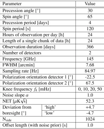
We have carried out several tests, considering a variety of offset lengths with and without a noise prior. For simulations, where we know the noise properties, it can be taken to be a priori known and exact; for real data it would be necessary to estimate the noise properties from the timeline data, although the accuracy of this estimate does not need to be especially high for typical applications (Natoli et al. 2002). For theCOREscanning strategy and the noise properties described in Table1, we found that the best MADAM performance is achieved for a offset of 1 s and using the exact noise prior (i.e. the description provided to the TOAST noise simulation tool).

4 Analysis of simulated noise maps

In this section we describe the noise maps produced with MADAM from timelines simulated with the TOAST pipeline described above. We analyse these maps to assess the robustness of theCORE scanning strategy in measuring the sky Stokes parameters with adequate purity. We also explore

4_{http://github.com/hpc4cmb/libconviqt}

Parameter Value

Precession angle [◦] 30

Spin angle [◦] 65

Precession period [days] 4

Spin period [s] 120

Hours of observation per day [h] 24 Length of a single chunk of data [h] 24 Observation duration [days] 366

Number of detectors 2

Frequency [GHz] 145

FWHM [arcmin] 7.68

Sampling rate [Hz] 84.97

Polarization orientation detector 1 [◦] -22.5 Polarization orientation detector 2 [◦] 67.5 Knee frequency fk[mHz] 0, 10, 20, 50

Noise slopeα 1.0

NET [µK√s] 52.3

Deviation from boresight [◦]

‘high’ +4.7

‘low’ -4.7

Nside 1024

Offset length (with noise prior) [s] 1.0

Table 1. Parameters supplied to TOAST to generate the baseline simulations. See text for details. The sampling rate is chosen to ensure four samples per beam FWHM.

possible tweaks to the scanning parameters to verify if they lead to increase robustness. Finally, we analyse the properties of the noise maps to find requirements on the detector knee frequency that ensure that residual contributions to the map on large angular scales are kept under control.

In Table1we summarize the parameters we selected as input to TOAST to produce the maps we analyse in this Section. More detail about the parameters in this Table and onCORE’s scanning strategy is given in de Bernardis et al.(2017)). We consider the COREbaseline scanning strategy with spin and precession angles of 65◦and 30◦respectively, with corresponding periods of 120 s and 4 days respectively. In this Section we consider timelines containing only instrumental noise. Signal contributions are examined in Sections6,7and8below. We simulate an entire year of observations divided into segments of 24 hours. These are then combined to produce the final map. This segment size is a reasonable compromise between the need to capture long timescale features in the noise and the desire to minimize computational and memory requirements. We assume a noise model with power spectrum density:

P(f)= A

"

fk f

!α

+1

#

­150°­120° ­90° ­60° ­30° 0° 30° 60° 90° 120° 150°

400 600 800 1000 1200 1400 1600 1800

­150°­120° ­90° ­60° ­30° 0° 30° 60° 90° 120° 150°

400 600 800 1000 1200 1400 1600 1800

Figure 2.Hit map for a pair of detectors located at the center of the focal plane after one year of observation. The map is shown in Ecliptic coordinates (left) and in Galactic coordinates (right). We also show (orange contours) an estimate of the polarization amplitude of the foregrounds at 70 GHz, a frequency close to the minimum emission of diffuse foregrounds. The outermost contour corresponds to 1.3µK in polarized intensity, and the subsequent contours to further steps of 1.3µK.

In the remainder of this Section we consider a pair of polarization sensitive detectors at 145 GHz at the same position in the focal plane, either at the boresight or at the edges of the focal plane, oriented at −22.5◦ and 67.5◦ with respect to the scan direction. This choice equalizes the noise power in theQandUStokes parameters and produces EE and BB angular power spectra with similar amplitude. In any case, any particular choice of orientation becomes irrelevant when producing maps from a large number of detectors, assuming their orientations are evenly spaced. We adopt these particular values for the sole purpose of achieving balance in the Stokes parameters in this minimal two-detector exercise. We also simulate the sky as observed by detectors at the edge of the focal plane. These are modelled by considering two pairs of detectors at±4.7◦with respect to the boresight along the direction orthogonal to the scan direction. These have the same polarization orientation as the boresight detectors and are labelled as ‘high’ and ‘low’ detectors in Table1and hereinafter.

The hit map for the two-detector case described above is given in Fig.2, having chosen a bore-sight direction. The irregular small-scale features, hardly visible at standard figure size, would be diluted when considering a larger number of detectors. From this simple exercise, we show that the CORE scanning strategy leads to a complete sky coverage in around 6 months, yet a coverage of around 45% of the full sky is achieved in just 4 days thanks to the wide precession. After one year, all pixels in the sky have been observed at least 200 times by a pair of detectors, assuming 3.4 arcmin pixels (HEALPix Nside =1024). The hit map in Galactic coordinates is overplotted with an estimate

of the total diffuse polarized foregrounds at 70 GHz, where emission is close to a minimum (Planck Collaboration et al. 2016b). This estimate was obtained using the Planck353 GHz and 30 GHz po-larized maps respectively as dust and synchrotron templates. This simple exercise shows how the COREscanning strategy provides high signal-to-noise sampling of regions that are remarkably clean of polarized foreground emission. Of course, the use of specific component separation techniques will reduce residual foreground emission considerably (Remazeilles et al. 2017).

­150°­120° ­90° ­60° ­30° 0° 30° 60° 90° 120° 150°

II

200 300 400 500 600 700 800 900 1000

­150°­120° ­90° ­60° ­30° 0° 30° 60° 90° 120° 150°

QQ

250 500 750 1000 1250 1500 1750 2000 2250

­150°­120° ­90° ­60° ­30° 0° 30° 60° 90° 120° 150°

II

200 300 400 500 600 700 800 900 1000

­150°­120° ­90° ­60° ­30° 0° 30° 60° 90° 120° 150°

QQ

300 600 900 1200 1500 1800 2100 2400 2700

­150°­120° ­90° ­60° ­30° 0° 30° 60° 90° 120° 150°

UU

250 500 750 1000 1250 1500 1750 2000 2250

­150°­120° ­90° ­60° ­30° 0° 30° 60° 90° 120° 150°

QU

600 450 300 150 0 150 300 450 600

­150°­120° ­90° ­60° ­30° 0° 30° 60° 90° 120° 150°

UU

300 600 900 1200 1500 1800 2100 2400 2700

­150°­120° ­90° ­60° ­30° 0° 30° 60° 90° 120° 150°

QU

600 450 300 150 0 150 300 450 600

­150°­120° ­90° ­60° ­30° 0° 30° 60° 90° 120° 150°

IQ

4.0 3.2 2.4 1.6 0.8 0.0 0.8 1.6 2.4 1e 13

­150°­120° ­90° ­60° ­30° 0° 30° 60° 90° 120° 150°

IU

4 3 2 1 0 1 2 3

1e 13

­150°­120° ­90° ­60° ­30° 0° 30° 60° 90° 120° 150°

IQ

5 4 3 2 1 0 1 2 3

1e 13

­150°­120° ­90° ­60° ­30° 0° 30° 60° 90° 120° 150°

IU

3 2 1 0 1 2 3 4

1e 13

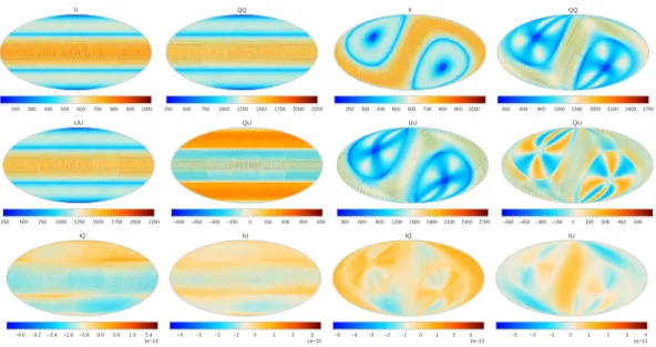
Figure 3. Elements of the white noise covariance matrix for a pair of boresight detectors displayed as maps in units of

µK2_{:II(top left),QQ(top right),UU(center left),QU(center right),IU(bottom left),IQ(bottom right). Coordinates are} Ecliptic (left columns) and Galactic (right columns). Notice thatIQandIUcorrelations are very weak.

the timeline. We set a limit of a minimum RCN of 10−2for the present analysis. We also compute the angular power spectra (APS) of the simulated noise maps. The noise APS allow to assess the destriping efficiency of MADAM in controlling spurious low-frequency contributions.

4.1 Baseline scanning strategy

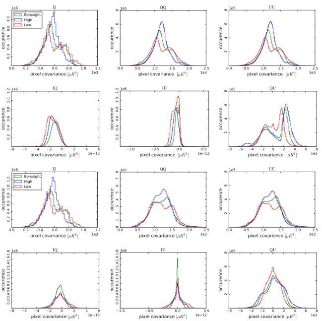
In Fig. 3 we show maps of the elements of the 3× 3 white noise covariance matrices produced by MADAM for the case of boresight detectors for both Ecliptic and Galactic coordinates, and his-tograms of these matrix elements are shown in Fig.4. Larger values of these histograms reflect larger pixel variance of the noise maps. An effective scanning strategy will achieve compact histograms with low mean values and minimal tails. These requirements are reasonably satified by CORE, as observed in Fig. 4: the histograms do not possess large tails, total intensity has smaller values with respect to polarization by a factor of 2, and the QQandUU histograms are very similar to one an-other. This last property is influenced by the particular choice of the orientations of the detectors as explained above. In addition, intensity and polarization show almost negligible correlations, while QUdoes show significant correlation features. These however are expected to vanish when a multi-detector map from an entire frequency channel is produced, in view of the large number of multi-detectors per frequency expected byCORE, and the desirable variation in mutual orientation (in fact, it would suffice to consider only four detectors with polarization angles at exactly 45◦to each other to have this correlation vanish).

As described above, a useful quantity for assessing the map-making inversion is the RCN. The RCN for the boresight solution is shown in Fig5. Reasonable requirements for optimal inversion are an average value across the histogram higher than 0.25 and no pixels with values lower than 10−2_.

0.0 0.2 0.4 0.6 0.8 1.0 1.2

pixel covariance [µK2_] 1e3

0.2 0.4 0.6 0.8 1.0 occurence 1e6 II Boresight High Low

0.0 0.5 1.0 1.5 2.0 2.5

pixel covariance [µK2_] 1e3

2 4 6 8 occurence 1e5 QQ

0.0 0.5 1.0 1.5 2.0 2.5

pixel covariance [µK2_] 1e3

2 4 6 8 occurence 1e5 UU

8 6 4 2 0 2 4 6

pixel covariance [µK2_] 1e 13

0.2 0.4 0.6 0.8 1.0 1.2 occurence 1e6 IQ

1.0 0.5 0.0 0.5

pixel covariance [µK2_] 1e 12

0.2 0.4 0.6 0.8 1.0 1.2 occurence 1e6 IU

8 6 4 2 0 2 4 6 8

pixel covariance [µK2_] 1e2

2 4 6 8 occurence 1e5 QU

0.0 0.2 0.4 0.6 0.8 1.0 1.2

pixel covariance [µK2_] 1e3

0.2 0.4 0.6 0.8 1.0 1.2 occurence 1e6 II Boresight High Low

0.0 0.5 1.0 1.5 2.0 2.5

pixel covariance [µK2_] 1e3

0 1 2 3 4 5 6 7 8 occurence 1e5 QQ

0.0 0.5 1.0 1.5 2.0 2.5

pixel covariance [µK2_] 1e3

2 4 6 8 occurence 1e5 UU

8 6 4 2 0 2 4 6

pixel covariance [µK2_] 1e 13

0.2 0.4 0.6 0.8 1.0 1.2 1.4 1.6 1.8 occurence 1e6 IQ

1.0 0.5 0.0 0.5

pixel covariance [µK2_] 1e 12

0.2 0.4 0.6 0.8 1.0 1.2 1.4 1.6 1.8 occurence 1e6 IU

8 6 4 2 0 2 4 6 8

pixel covariance [µK2_] 1e2

2 4 6 8 occurence 1e5 QU

Figure 4.Histograms of the 3×3 pixel covariance matrix elements in Ecliptic coordinates (first and second rows) and in Galactic coordinates (third and fourth rows). There are minimal intensity-to-polarization couplings (notice the change of scale) but significantQUresidual correlation.

mentioned that we have investigated the ideal performance of the scanning strategy here, neglecting, for example, cross-polar leakage.

In Fig.4we also show the histograms of the noise covariance matrix for the high (blue) and low (red) detectors. One of the risks for detectors at the edge of the focal plane is not achieving complete sky coverage. This is avoided by imposing the condition that the sum of the spin and precession angles is more than 90◦ for the entire focal plane. InCORE, the sum of these angles for the low detectors is 90.3◦ allowing for the complete sky coverage across the whole focal plane. We have used these simulations to verify that this is indeed the case. The histogram shapes are similar to the boresight ones, and there are no anomalous values of the noise covariance matrix elements. In Fig.

0.1 0.2 0.3 0.4 0.5 RCN 0 2 4 6 8 occurence 1e5 Boresight High Low

Figure 5.Histograms of the reciprocal condition numbers for the boresight, high and low detectors.

101 ₁₀2 ₁₀3 ` 0 1 2 3 4 5 C

TT `[

µK 2] 1e 3 Baseline High Low

101 ₁₀2 ₁₀3 ` 0 1 2 3 4 5 6 7 C E E ` [ µK 2] 1e 3

101 ₁₀2 ₁₀3 ` 0 1 2 3 4 5 6 7 C B B ` [ µK 2] 1e 3

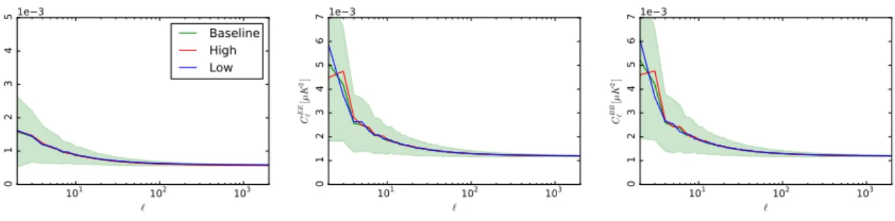
Figure 6. Angular power spectra forT T(left),EE(centre) andBB(right) of the baseline simulations for the boresight, high and low detectors. We show the average of 1000 simulations and the 1σdispersion for the boresight case (shaded regions).

Low detectors show slightly higher RCN, high detectors show slightly lower RCN. This allows us to extend the above conclusions about the clean separation of the Stokes parameters to the whole focal plane.

In Fig.6we show the averageT T,EEandBBAPS from 1000 noise realizations for the bore-sight, high and low detectors (details of our Monte Carlo pipeline are given in Appendix A). We also show the 1σdispersion of the boresight case. As already noted for the RCN, the APS of different detectors are all similar. The APS of low detectors show slightly lower amplitudes than the other two. TheEE andBBamplitudes are practically the same as a result of the choice of the polarization orientations. All spectra show a large scale (low multipole) excess, due to residual 1/f contribution after destriping. The impact of different knee frequencies is discussed in Section4.3.

4.2 Optimizing the scanning strategy

We investigate possible optimizations of theCOREscanning strategy by analysing the effect of vary-ing the spin angle and the precession angle. We consider seven pairs of values keepvary-ing the sum of these angles equal to 95◦ for the boresight detectors in order to preserve full sky coverage for the entire focal plane. In this way we define seven ‘tweaked’ cases to be compared to the baselineCORE scanning strategy (see Table 2 for the chosen values, all the other parameters are the same as in Table1).

Parameter Baseline Tweak 1 Tweak 2 Tweak 3 Tweak 4 Tweak 5 Tweak 6 Tweak 7

Precession angle [◦_{] 30 32 34 36 38 40 45 50}

Spin angle [◦

] 65 63 61 59 57 55 50 45

Table 2. Parameters modified with respect to Table1to obtain tweaked cases to evaluate a possible optimization of the COREscanning strategy. The first column gives the baseline parameters.

0.1 0.2 0.3 0.4 0.5

RCN 0 1 2 3 4 5 6 7 8 9 occurence 1e5 Baseline Tweak 1 Tweak 2 Tweak 3 Tweak 4 Tweak 5 Tweak 6 Tweak 7

0.1 0.2 0.3 0.4 0.5

RCN 0 1 2 3 4 5 6 7 8 9 occurence 1e5

0.1 0.2 0.3 0.4 0.5

RCN 0 1 2 3 4 5 6 7 8 9 occurence 1e5

Figure 7. Histograms of the RCN for the boresight (left), high (centre) and low (right) detectors in the tweaked cases compared to the baseline (cyan). The vertical dotted lines show the mean values.

101 ₁₀2 ₁₀3 ` 0.0 0.5 1.0 1.5 2.0 2.5 3.0 C

TT `[

µK 2] 1e 3 Baseline Tweak 1 Tweak 2 Tweak 3 Tweak 4 Tweak 5 Tweak 6 Tweak 7

101 ₁₀2 ₁₀3 ` 0.0 0.2 0.4 0.6 0.8 1.0 1.2 C E E ` [ µK 2] 1e 2

101 ₁₀2 ₁₀3 ` 0.0 0.2 0.4 0.6 0.8 1.0 1.2 C B B ` [ µK 2] 1e 2

Figure 8.T T(left),EE(centre) andBB(right) APS of the baseline simulations for the boresight detectors compared to the tweaked cases described in Table2.

average RCN is slightly lower. Cases 6 and 7 show slightly improved RCN with respect to the baseline especially for the boresight detectors. The improvements are less evident when the high and low detectors are considered. The highest mean RCN is achieved by case 6 with a value of about 0.42 for the boresight detector which, given the dispersion of the RCN values shown in Fig.7, is not significantly different from the 0.41 achieved by the baseline, in view of the generous spread of RCN values. This is a small improvement that would require significant changes in spin and precession angles, and would have negative impacts on other subsystems of the spacecraft (for example, a lower power supply due to the change in solar aspect angle).

In Fig.8we show the APS of the noise maps for the boresight, high and low detectors. All the APS here are the result of the average over 10 noise realizations. The APS of the tweaked cases are compared to the baseline and its 1σdispersion delimited by the cyan shaded region. At small scales the APS are all almost identical. Larger differences are evident at large scales, but they are well inside the 1σdispersion.

101 ₁₀2 ₁₀3 ` 0 1 2 3 4 5 C

TT `[

µK

2] 1e 3

fknee=0mHz fknee=10mHz fknee=20mHz fknee=50mHz

101 ₁₀2 ₁₀3 ` 0.0 0.2 0.4 0.6 0.8 1.0 1.2 C E E ` [ µK 2] 1e 2

101 ₁₀2 ₁₀3 ` 0.0 0.2 0.4 0.6 0.8 1.0 1.2 C B B ` [ µK 2] 1e 2

Figure 9. T T(left),EE(centre) andBB(right) APS of the baseline simulations for the boresight detectors considering several knee frequencies fk. We show the APS from the boresight detectors (solid lines), high detectors (dotted lines) and

low detectors (dashed lines).

4.3 1/f noise performance

In this Section we investigate the effect of the low frequency noise properties. We simulate a year of observations for a pair of boresight, high or low detectors considering several knee frequencies fkin the range between 0-50 mHz, a range that appears reasonable in view ofCORE’s planned detectors. As mentioned above, we make use of a noise prior in MADAM, which requires as input an estimate of the noise power spectral density. We provide here the true underlying power spectrum of the noise. Even if this may be considered an optimistic choice, in practice the impact on the results of a mismatch between the true and estimated noise properties is weak, as noted in Sect.3above. We always use 1 s as the MADAM offset length. We generate 1000 Monte Carlo (MC) realizations (see Appendix A) and apply MADAM to produce noise-only maps. The amplitude of residuals can be turned in a requirement on the maximum acceptable knee frequency.

In Fig. 9 we show the average APS from 1000 MC realizations for the knee frequencies fk of 10 mHz (red line), 20 mHz (blue line), 50 mHz (black line). They are compared with the pure white noise case fk = 0 mHz and its 1σ dispersion (cyan line and shaded region). In the same Figure we show the results for a pair of low detectors (dashed lines) and high detectors (dotted lines). As expected, we do not observe any difference between the position of the detectors in the focal plane. The effect of the destriping residuals is a larger amplitude of the noise spectrum at large scales (` < 100) and, as expected, the residuals increase with increasing fk. The 10 mHz case lies at the edge of the 1σdispersion of the white noise MC. Knee frequencies lower than this value will generate noise maps that cannot be practically distinguished from pure white noise both in temperature and polarization. Therefore low frequency noise drifts have negligible effects if fk < 10 mHz. We notice that a knee frequency of 20 mHz is still an acceptable compromise showing an increase in the noise APS mostly confined to` <10.

con-101 ₁₀2 ₁₀3

Multipole`

10

−

6

10

−

5

10

−

4

10

−

3

10

−

2

10

−

1

10

0

10

1

10

2

`

(

`

+

1)

C`

/

2

π

[

µ

K

2]

r=0.1

r=0.01

r=0.001 CORE miniCORE

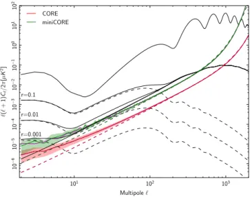
Figure 10. Polarized noise angular power spectra (coloured lines) inEEandBBforCORE(red and blue lines respec-tively) andminiCORE(magenta and cyan respectively), considering all channels between 130 and 220 GHz, compared to EEandBBCMB theoretical spectra for several values of the tensor-to-scalar ratior(the solid curve includes lensing B modes). The shading corresponds to the 1σuncertainty region. See text for details.

sidered in theCORE cosmological parameters and inflationary forecasts discussed inDi Valentino et al.(2016) andCORE Collaboration et al.(2016).

Results are shown in Fig.10, where they are compared toEEandBBCMB spectra, considering for the latter several values of the tensor to scalar ratio r, while the other cosmological parameters are kept to the Planck 2015 updated best fit values (Planck Collaboration et al. 2016g). The red dashed line shows the noise spectrum from the inverse noise weighting of the six CMB channels as described above. The solid line shows noise APS of a pair of detectors as result of the average of 1000 noise realizations (assuming fk = 50 mHz and a beam of 5 arcmin), rescaled to match the dashed line at ` = 300. We show bothEE (blue line) and BB(red line) spectra although they are almost indistinguishable. We also show the 1σdispersion of the realizations as the shaded region. The effect of 1/f noise is noticeable at`.100. However, even in this pessimistic assumption of fk =50 mHz, the noise spectrum is well below theBBspectrum forr=10−3_{for`.10. We also show in Fig.10the}

forecasted noise spectra (magenta forEE, cyan forBB) for the so-calledminiCOREdesign, a down-scoped configuration ofCORE(seede Bernardis et al.(2017) for more detail). We follow the same approach described above, but consider theminiCOREparameters for the beam FHWM (11.9 arcmin at 145 GHz, corresponding to a sampling rate of 54.8 Hz) and averaging over 10 noise realizations instead of 1000. All the other parameters, except of course the number of detectors per channel, are identical toCORE(see table1). Despite the noise level forminiCOREis now significantly closer to theBBspectrum forr =10−3, this design still allows plenty of margin for an accurate measurement of tensor modes in view of 1/f residual contamination, especially considering that fk = 50 mHz is taken here as a worst case scenario.

5 Cross-correlated noise

forth-coming generation of CMB experiments. The presence of these common modes is usually neglected during analysis, though optimal treatment can easily be included in the GLS framework discussed in Sect.2, at the cost of increasing the computational burden (de Gasperis et al. 2016;Patanchon et al. 2008), as detailed in Appendix B. In short, a solution formally identical to Eq.2.3 can be obtained for the the estimated mapme:

e

m=ATN−1A−1ATN−1d, (5.1) where dand Aare respectively a multi-detector timeline and pointing matrix and Na generalized noise matrix:

N≡ hntnt0i=

              D

n(1)_t n(1)_t0

E

· · · Dn(1)_t n(_t0k)

E

... ... ...

D

n(_tk)n(1)_t0

E

· · · Dn(_tk)n(_t0k)

E               , (5.2)

whereh·idenotes the expectation value and (·) labels different channels. As is customary, we assume stationary noise, implying that the statistical properties of the noise do not change over the mission lifetime. To be specific, when considering the j-th and`-th detectors and the noise elements n(<sub>t</sub>j) andn(<sub>t</sub>`0)at time tandt0, respectively, we assume that

D

n(_tj)n(_t`0)

E

only depends on |t−t0|. Moreover, we consider that the noise statistical properties are known and completely described by the noise covariance matrix. We assume that the noise auto- and cross-spectra can be estimated either by on-ground instrument calibration or directly from observational data by dark-sky measurements or iterative procedures (see e.g.Prunet et al. 2001).

To findme, the optimal GLS formula can be solved iteratively using a Fourier based,

precon-ditioned conjugate gradient method as outlined in Sect. 2. Note however that, given the full noise covariance matrix (whose effective size is proportional to N+Nc ×(Nc −1)/2, where N is the to-tal number of detectors and Nc is the number of with cross-correlated noise), a single iteration of the preconditioned conjugate gradient solver scales linearly with the total number of samples, but quadratically withNc.

We set up aCOREtest case by generating a noise timeline with the TOAST software assuming theCOREscanning strategy and detector parameter baseline (see Tab.1), considering the cases of 2 and 4 detectors for 1 year of operations. Following the behaviour ofPlanckHFI (Planck Collabora-tion et al. 2016g), we assume that the noise of thei-th detector has the following properties:

ni = n˜i+nc (5.3)

Pi(f)≡ hn˜in˜ii = A

" fk f ! +1 # (5.4)

Pi j(f)≡Dninj

E

=hncnci = A

       f₁ f !2 +C      

fori, j (5.5)

where ˜ni andncrefer to the self- and cross-correlated noise component, with knee frequencies fk = f₁ =20 mHz. We assumeC=0 and use the NET from Table1for the amplitudeA. We then generate noise maps with:

1. a GLS map-making algorithm that considers only the diagonal terms of the noise covariance matrix that correspond to the auto-correlated 1/f noise (the ROMA MPI-parallel code, see

Natoli et al. 2001andde Gasperis et al. 2005);

For each case above, we generate the noise-only maps of the Stokes parameters QandU. In Fig.11

we show the difference of the noise-onlyQandU maps between the cases with and without cross-correlated noise in the map-making code (for the 2 detector case). These difference maps show stripy structures, suggesting that the inclusion of the cross-correlation properties in the noise model mitigates the residual correlation along the scan. We then compute the r.m.s. values of the maps, noting very slight differences between cases 1 and 2 above (of few parts out of 104). However, it should be emphasized that the map r.m.s. is not the most appropriate figure of merit here, since the effect of accounting for the noise cross-correlation is limited only to the very large angular scales. An APS analysis is better suited inasmuch as it separates the contribution of different angular scales. We therefore produce 20 Monte Carlo noise-only maps and generate the corresponding APS. We then compare the average spectra for cases 1 and 2 above by calculating their ratio (see Fig.12). We notice that neglecting the noise cross-correlation results in a larger noise amplitude at very large angular scales. This excess is suppressed by accounting for the detector cross-correlation in the map-making: in fact, we have a decrease of the noise spectrum amplitude up to 5-10% at very low multipoles. Finally, we compare the APS standard errors as computed from the the dispersion of the simulated Monte Carlo maps (see Fig.12). We find that the inclusion of the cross-correlated noise provides smaller error-bars at the largest angular scales (again, up to 5-10%), while, as expected, we do not find any relevant difference at smaller scales.

Results shown in Fig.12 correspond to the 2 detector case. Tests on the 4 detector case have shown the same qualitative behaviour: we still find a decrease in both noise spectrum amplitude and standard deviations of 5-10% after including the noise cross-correlation information in the map-making process. We emphasize that the common-mode noise contribution does not easily integrate down with increasing the number of detectors, as opposite to the auto noise component. For this reason, the noise cross-correlation should be carefully accounted for in any polarization experiment with a large number of detectors, and the map-making process is the natural place to deal with it.

We emphasize that the amplitude of this effect is not straightforward to forecast accurately (as it will crucially depend of the instrumental set-up), but we highlight the importance of having a pipeline able to handle it. Indeed, our analysis shows that the effect of the noise cross-correlation is not negligible. Due to the faintness of the B-mode polarization signal, the improvement provided by the extended map-making algorithm may prove crucial for accurate characterization of such contribution at the largest angular scales: accurate modelling of noise at low resolution is an important task to reliably measure the B mode reionization bump, since for some highly efficient estimators devoted to this task noise misestimation may induce bias (Mangilli et al. 2015), contrary to what happens for GLS map-making.

6 Bandpass mismatch

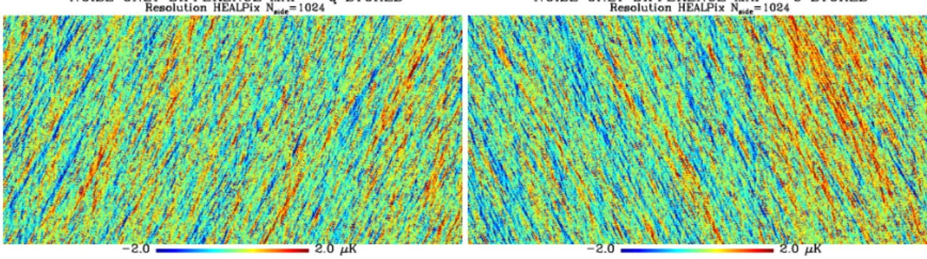
strat-Figure 11.Difference of the noise-only maps of the Stokes parametersQ(left) andU(right) between the cases accounting for and ignoring cross-correlated noise in the map-making (Cartesian projection). Maps have been estimated assuming 2 detectors and one year of operation. Maps are in Ecliptic coordinates, in units ofµKand at resolution HEALPixNside=1024

(3.435 arcmin/pixel). The stripes are due to the cross-correlated noise, which is mitigated when it is taken into account in the map-making algorithm.

EE

-20 -15 -10 -5 0 5 10

Fractional difference (%)

10 100

Multipoles 0

1 2 3 4 5

Stand. dev. [10^(-3) uK^2]

BB

-20 -15 -10 -5 0 5 10

Fractional difference (%)

10 100

Multipoles 0

1 2 3 4 5

Stand. dev. [10^(-3) uK^2]

Figure 12. Comparison ofEEandBBangular power spectra between the cases accounting for and ignoring the cross-correlated noise in the map-making algorithm. Spectra have been estimated from 20 noise-only Monte Carlo realizations, assuming 2 detectors and one year of operation. On the top: fractional difference ofEE(left) andBB(right) average spectra between the two cases. On the bottom: EE(left) andBB(right) spectrum standard deviations of the cases accounting for (dashed red line) and ignoring (solid black line) cross-correlation. Standard deviations correspond to the dispersion of the simulations.

6.1 Model of the bandpass mismatch effect

As discussed in Sect. 2(see in particular Eq.2.2), a detector observing the sky at the frequency ν0

with a polarizer oriented at an angleψtat timetmeasures the quantity:

dt(ν0)=Ip(t)(ν0)+Qp(t)(ν0) cos (2ψt)+Up(t)(ν0) sin (2ψt)+nt, (6.1) whereIp(t)(ν0),Qp(t)(ν0) andUp(t)(ν0) are the Stokes parameters at the position p(t) on the sky

mea-sured in the local reference frame andntis the random instrumental and photon noise.

For a given sky pointing, each of the Stokes parameters (I,Q,U) receives contributions due to the emission of different componentsc. For simplicity, let us model the intensity in terms of these components. After integrating over the detector bandpass, the total flux par unit steradian received by a detector from the sky can be written as (seeHoang et al.(2017) for details on this model):

dF dΩ =

Z X

c

g(ν)fc(ν,p)dν, (6.2)

where g(ν) is the detector bandpass, fc(ν,p) the emission spectrum of thec component, which can depend on the pixel. After calibrating on the CMB, the intensity reads:

I(ν0)=ICMB(ν0)+ X

c_,CMB

γc(p)Ic(ν0), (6.3)

whereIc(ν0) is the mean intensity of componentcat a reference frequencyν0andγc(p) the relative

amplitude of componentcin CMB temperature units, which is slightly pixel dependent if the compo-nent spectra depend on the sky region considered. Since the signal has been calibrated on the CMB, the factorγCMBis normalized to unity. The component amplitude coefficient, defined for the

refer-ence frequencyν0, can be related to the transmission of the band and the spectrum of the component

by:

γc=

R

g(ν)fc(ν)fc(ν0)−1dν R

g(ν) dB(ν,T0)

dν

_ν

0 dν

dB(ν,T0) dν

ν

0

, (6.4)

whereT0is the mean temperature of the CMB and B(ν,T0) is the blackbody spectrum of the CMB.

The quantityγcis close to 1 for a chosenν0near the center of the band. A similar relationship applies

for theQandUStokes parameters.

The expression above describes an ideal situation and does not include real-world complica-tions such as beam asymmetries and miscalibration. We follow this approach in order to isolate the bandpass mismatch effect. Potential couplings with other systematic effects are ignored at this stage, in the spirit of the discussion in Sect.1.

The problem of bandpass mismatch can be understood by calculating the data model for the sky signal for a set of detectors{(i)}. Each detector (i) in the set will have its ownγ(ci) which can be written as

γ(i)

c =γc+δγ

(i)

c (6.5)

where γc is the mean of scaling parameter γ for the set {(i)} and the component c and δγ

(i)

c is its deviation from this mean. The data model for the sky signal can now be written, using a vector notation in boldface, as

d(i) = X

c γ_c

Ic+Qccos (2ψ)+Ucsin (2ψ)+

X

c,CMB

δγ(i)

The first term on the right hand side is the ‘ideal’ sky signal with all components including CMB, while the second term is the leakage term of non-CMB components due to their different bandpasses. Since the signal for each detector has been calibrated on the CMB, we expectδγC MBto be zero, so it is absent from the second term.

6.2 Simulations of the bandpass mismatch effect

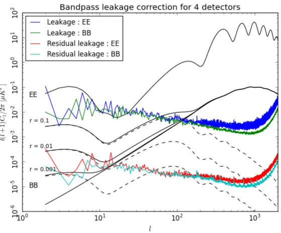
We evaluate the impact of the mismatch on a set of simulations of the data using a simplified version of thePlancksky model (PSM, seeDelabrouille et al.(2013)), which comprises only two foreground components (thermal dust and synchrotron) and CMB at 145 GHz, at HEALPix resolution N_side = 1024, and symmetric Gaussian beams of FWHM 7.60. We use four detectors, with polarization angles evenly spaced at intervals of 45◦, at the boresight, and with varying square bandpasses with a 1% random error on the edge of the bands. This gives similar variations of theγparameters than for the most pessimistic cases of Planckfilters. Nevertheless, we expect less variations between future mission detector filters. The sky component is integrated over the corresponding spectrum following Eq. 6.4, using a top hat instrumental bandpass. In simulations, we have included the complexity of component spectra as modelled in the PSM, and consequently the resulting γ parameters are pixel dependent. We have run simulations of pure signal and of signal plus white noise separately, using the nominal noise level expected forCORE, observing for one year using the baselineCOREscanning strategy as discussed in Sect.4above.

As described in Sect.2, we produce intensity and polarization maps using the maximum like-lihood estimator for the Stokes parameters, Eq. (2.3). In the first step we ignore the correction for bandpass leakage and use the same pixelization as the input maps to avoid introducing additional pixelization effects. Maps of the timeline noise are made separately and subtracted from total maps. This is justified since the map-making method which has been used is linear, and so instrumental noise will be purely additive.

In the absence of bandpass leakage, that is, if allγ(ci), for each detector (i) are identical, and there is sufficient modulation of the polarization angleψ, we expect Qcp = Qp andUcp = Up, the actual signal on the sky with no additional bias, for all pixels given our noiseless simulations.

By comparing the resulting polarization maps with the input, we estimate the impact of band-pass leakage on the polarization measurement for the chosen detector set. We compute theQbandUb

maps and compute theEEandBBpower spectra of the difference with the input CMBQandUmaps after masking 25% of the sky where the Galactic dust emission is the brightest. The resulting power spectrum of the residual signal (see Fig.13) is above the primordialB-mode signal even forr=0.1, and is thus completely unacceptable for measuring r = 0.001. It is also above the lensing signal for ` < 100 (see, again, Fig 13). The prediction for any number of detectorsN_det can be obtained by rescaling the power spectrum of a factor 4/Ndet(since the result described here is for four

detec-tors), assuming independent filter variations between detectors. The scaling of the spectrum with the inverse of the number of detectors is demonstrated inHoang et al.(2017).

6.3 Correction algorithm

more generalized correction algorithm based on the model of the data introduced in the last section and describe the simulation employed to validate it.

The baseline focal plane design for the COREmission uses detectors with dual polarization sensitivity in one single focal plane pixel, as well as pairs of single polarization detectors with or-thogonal polarization sensitivity scanning the sky along the same trajectory. The former can directly be differenced to cancel intensity and get a polarization signal, while the latter can also be diff er-enced but after correcting for the appropriate time-shift. Differencing in this way the timelines of two orthogonal detectors, we obtain

d=1

2

d(a)−d(b)

= X

c γ_c

Qccos (2ψ)+Ucsin (2ψ)+ 1 2         X

c,CMB

δγ(a)

c −δγ( b) c Ic        +

n(a)−n(b)

=Qcos (2ψ)+Usin (2ψ)+ X c,CMB

ycIc+n, (6.7)

and we are left with a reduced set of Stokes parameters [Q,U] from the CMB and Galactic sources,

Icare the timelines from reference foreground intensity maps withyc their corresponding amplitude, each of them given by 1₂δγc(a)−δγ(

b)

c

, andnis the noise term.

In equation6.7, the first term on the right hand side is the term of interest (a linear combination of the polarization Stokes parameters), while the other two are nuisance terms, a bandpass leakage term proportional to a sum of foreground components, and a noise termn.

By recasting our data set in the form of equation6.7, we have isolated a leakage term which is a sum of bandpass mismatch coefficients times foreground intensity templates. If the bandpass mismatch coefficientsyc are perfectly known by calibration, our measurements can be considered as linear combinations of P

Q_c (sky Stokes Q in channel c), P

Uc (sky Stokes U in channel c), and additional foreground intensity mapsIc. The system can be inverted in the usual way. If however the calibration of the bandpasses is not perfect, we want to solve also foryc.

We propose to correct for bandpass mismatch terms with the following approximation. Assume that we have at hand measured templates for the foregrounds. Such measurements can be obtained directly forCOREintensity data, either at other frequency (i.e. higher frequency for a dust template, or lower for a synchrotron template), or at the reference frequency of the channel of interest after component separation in intensity. Such templates are not perfect, i.e.

Ic =keIc+δIc, (6.8)

where k is a global scaling factor, andδIc the difference between the scaled template and the real foreground map. By replacing the (unknown)Icby its expression in terms of the (known) templatebIc in Eq.6.7, neglecting the second-order term proportional toycδIc, and absorbing the global scaling factorkinyc, we get, in matrix-vector notation

d=Am+Ty+n, (6.9)

where A is a reduced pointing matrix with has two non-zero elements in each row

At p(t) = h

cos (2ψt) sin (2ψt)

i

, (6.10)

mis the reduced set of Stokes parameters, containing only [Q,U] from both the CMB and the Galactic sources, Tis built from the knownforeground template mapseIc, y is the set of amplitudes of the

We find an unbiased estimator me free (to first order) from the leakage term with a standard

generalized least square estimator of the form

e

m=ATN−1FTA

−1

AN−1FTd, (6.11)

ey=

TTN−1FAT

−1

TN−1FAd, (6.12)

and

FA=

1−AATN−1A−1ATN−1

, (6.13)

FT=

1−TTTN−1T−1TTN−1

. (6.14)

We identify the termsFAandFTas operators that filter out the component of the signal in the

respective space ofAandT. Also, the noise covariance termNfor the case of white noise is diagonal given byσ21, whereσis the standard deviation of the white noise, and it cancels out in the previous equations. We thus freely drop the noise covariance termN. It is to be noted that this algorithm can be suited for any number of systematic effects whose leakage signal can be modelled as a nuisance term proportional to a temporal template as shown in equation (6.7). An analogous approach to subtract temporal templates was implemented inPoletti, D. et al.(2017) for the Polarbear experiment using the direct estimation of maps as in equation (6.11).

To make matters computationally feasible we perform our correction iteratively by first esti-mating the amplitudesyof the templates using Eq. (6.12), then use these to perform a simple GLS map-making by subtracting the leakage term from the timeline by

e

m=ATA−1AT d−T_ey

(6.15) We test here this correction algorithm on the simulations described in the previous subsection. For our templates we simulate intensity maps for thermal dust at at 350 GHz and synchrotron at 90 GHz using the PSM. TheEEandBBpower spectra of the leakage maps are shown in Fig.13. The algorithm reduces the leakage by more than two orders of magnitude in power. The residual after correction for a set of 4 detectors is now comparable to the primordial B-modes for a level ofrin the 0.001-0.01 range, and below the lensing signal for`≥10.

As already emphasized, the power spectrum of the leakage after averagingNpairs of detectors will be reduced by N. TheCORE145 GHz channel comprises 144 detectors (72 pairs). Hence we estimate that the residual leakage after correction and averaging all detectors of the channel will be one order of magnitude or more below the target sensitivity at all angular scales. If necessary, this approach can be extended to second order to further reduce the residuals.

7 Asymmetric beam

The convolution of the CMB signal with an asymmetric beam will cause leakage between intensity and andE- andB-mode polarization whenI,QandUmaps are reconstructed using the generalized least squares solution of equation2.3without proper measures to take into account this beam asym-metry. Given that the primordial intensity signal is much larger than the polarization signal, the most important effect is the temperature-to-polarization leakage.