Sharif University of Technology
Scientia IranicaTransactions A: Civil Engineering http://scientiairanica.sharif.edu
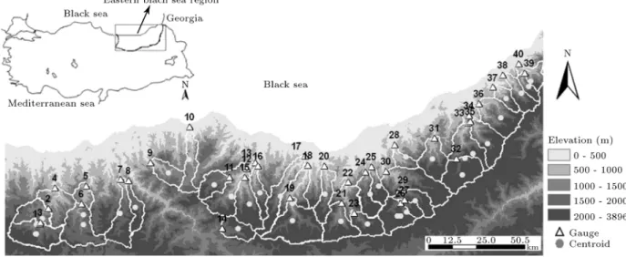
Streamow map of the Eastern Black Sea Region,
Turkey
E. Eris
a;and N. Agiralioglu
b,1a. Department of Civil Engineering, Ege University, Bornova, Izmir, 35100 Turkey.
b. Hydraulics Laboratory, Faculty of Civil Engineering, Istanbul Technical University, Maslak, Istanbul, 34469 Turkey. Received 4 February 2016; received in revised form 14 September 2016; accepted 14 January 2017
KEYWORDS Streamow map; Ordinary kriging; Universal kriging; Simple regression; Eastern Black Sea Region.
Abstract. The purpose of this study is to generate a streamow map for the coastal part of the Eastern Black Sea Region, which is located in the north-east of Turkey. The topographic structure of the region is an obstacle in terms of the number of observation gauges. In order to determine spatial variation of ow and to estimate ow on any ungauged points in the region, interpolation between gauged and ungauged points is applicable. For this purpose, any hydrological models, which depend on large meteorological datasets, can be used. However, in this study, ordinary and universal kriging as geostatistical interpolation methods are used to interpolate mean annual ow depth over the study area; thus, ow values on ungauged points can be easily estimated. Kriging methods are compared with simple regression based on the relationship between ow data and basin area. Calibration results of the observed and estimated ow depths for ordinary and universal kriging methods are satisfactory; the determination coecients are found to be 0.84 and 0.87, respectively. Besides, the validation results show that the performance of kriging methods is superior to that of the regression model.
© 2018 Sharif University of Technology. All rights reserved.
1. Introduction
Spatially distributed hydrological models provide more cost-eective means for determining water potential assessment within a basin; however, the accuracy of model results strongly depends on the accuracy of model inputs, particularly precipitation observations. In mountainous regions, most of the precipitation observations usually have 30% or higher error, whereas streamow errors vary from 5% to 10%-15% [1]. In addition, the number of observation gauges is limited
1. Present address: Department of Civil Engineering, Antalya Bilim University, Antalya, 07190, Turkey
*. Corresponding author. Tel.: +90 232 3115041; Fax: +90 232 3425629
E-mail addresses: [email protected] (E. Eris); [email protected] (N. Agiralioglu) doi: 10.24200/sci.2017.4261
in developing countries. Besides, in cases where spatial streamow estimation for longer periods such as monthly, seasonal, or annual scale is required, simpler relationships may prove sucient approximation [2]. In order to avoid the complexity of hydrological models, which depend on accurate and large meteorological dataset, available ow observation data can be used for determining spatial variation of streamow.
Spatial variability of ow has been represented by various techniques. For instance, ow depth has been dened as a regionalized phenomenon that uses a centroid based method by performing ordinary krig-ing to predict long-term streamows correspondkrig-ing to dierent exceedance probabilities over space and time [2]. The method locating gauged ow values at the centroids of the basins has previously been used for runo mapping [3-5]. This approach has also been used for ood regionalization [6]. The main idea in this study is that spatial proximity is a signicantly
better estimator of regional ood frequencies than basin attributes are.
The total area in mapping can sometimes be di-vided into fundamental units, i.e. sub-dividing a larger basin into sub-drainage basins or into a regular grid network. The drainage basins can be dened by points in space and, during the mapping processes, average of the runo from all the sub-drainage basins that fall within a grid cell is used. A disadvantage of this method is that some cells do not include observation points. To overcome this problem, a deterministic interpolation is applied and used as the Triangulated Irregular Network (TIN) technique (i.e., linear interpo-lation within the TIN facets, represented by the gaug-ing station, which has been considered as nodes) [7].
Other studies are based on disaggregation and covariance approaches [8,9]. These approaches were developed for mapping annual runo along the river network using water balance constraints in the es-timations [10]. They were subsequently extended, generalized, and applied to mean annual runo coupled with empirical relations presented by an application to assess water resources in France [11]. Eects of local features such as karst and river regulations were then added into this approach to produce the maps of mean runo for France [12].
Top-kriging (topological kriging) was presented in ungauged catchments [13] as a method to esti-mate streamow-related variables. The concept was built [10] and extended in a number of ways. Although the method was tested for the 100-year ood case in two Austrian regions, it can be used to spatially interpolate a range of streamow-related variables such as mean annual ow, low ow, and ood characteristics, and it provides more robust estimates than regional regression models do [14]. Top-kriging has recently been used to estimate ood quantiles and ow duration curves for
ungauged sites and has been compared with canonical kriging and regression equations [15,16]. Block kriging was coupled with water balance and data uncertainty analyses to estimate mean annual runo for a large basin in China [17].
In this study, the aim is to determine spatial variation of ow for the coastal part of the Eastern Black Sea Region, Turkey, as such a study is not avail-able for the region. Considering that the region has a signicant hydropower potential [18], it is important to know the ow at ungauged points. The coastal part of the Eastern Black Sea Region is mountainous such that most of the precipitation observation stations are located in the valley oors and they could not represent orographic precipitation characteristics of the region [19]. Because of this, use of any hydrological model based on precipitation data is not convenient to determine ow variability in the study area. In order to produce a streamow map, a previous study [2], which is based on kriging application for dierent exceedance probabilities of streamow estimation, is followed. The dierence of this study from the previous one is the use of mean annual ow observation data instead of ow data corresponding to dierent exceedance probabilities. Besides, this study includes a universal kriging application to produce streamow map for the coastal part of the Eastern Black Sea Region.
2. Study area and data
The study area is the coastal part of the Eastern Black Sea Region, which is situated in the north-east of Turkey, between the coordinates 40310-41240 North
and 38080-41260 East. This coastal part can be
dened as the region between the Eastern Black Sea Mountain chain and the Black Sea (Figure 1). The Eastern Black Sea Mountain chain is parallel to the
Table 1. Area and elevation of the ow gauges.
No Gauge
name
Area (km2)
Elevation (m)
Record period No
Gauge name
Area (km2)
Elevation (m)
Record period
1 Ikisu 317.2 1037 1986-1999 21 Alcakkopru 243 700 1979-2005
2 Alancik 470.2 700 1986-2004 22 Ulucami 576.8 260 1979-2005
3 Ikisu 292.7 990 1965-1974 23 Serah 154.7 1170 1966-2001
4 Dereli 713 248 1962-2004 24 Yenikoy 171.6 470 1982-2004
5 Tuglacik 397.9 400 1986-2006 25 Cevizlik 115.9 400 1982-2002
6 Sinirkoy 296.9 650 1983-2005 26 Toskoy 223.1 1296 1965-2002
7 Hasanseyh 256.8 370 1984-2006 27 Toskoy 284.3 1210 1986-2001
8 Suttasi 124.9 188 1970-2004 28 Komurculer 83.3 250 1984-2002
9 CucenKopru 162.7 240 1980-2006 29 Derekoy 445.2 942 1966-2002
10 Bahadirli 191.4 17 1962-2002 30 Simsirli 834.9 308 1988-2004
11 Ormanustu 150 770 1985-1999 31 Kaptanpasa 231.2 480 1984-2006
12 Kanlipelit 708 257 1951-1989 32 Cat 277.6 1250 1982-1999
13 Ogutlu 728.4 160 1984-2004 33 Konaklar 496.7 300 1980-2005
14 Ikisu 149.6 1450 1984-1999 34 Topluca 762.3 233 1964-2002
15 Ortakoy 261 380 1980-2002 35 Mikronkopru 239.2 370 1980-2004
16 Ciftdere 121.5 250 1980-2006 36 Kemerkopru 302.2 230 1984-1997
17 Findikli 258.6 90 1979-2004 37 Arili 92.15 150 1982-2005
18 Agnas 635.7 78 1944-2002 38 Koprubasi 156 60 1966-2003
19 Aytas 421.2 510 1979-2005 39 Kucukkoy 66.37 310 1985-2006
20 Ortakoy 173.6 150 1979-2006 40 Baskoy 186.2 75 1978-2006
coast as the north boundary of the study area, and it rises to more than 3000 m above msl (mean sea level). The Black Sea Region has a rocky steep coast [20].
Humid and mild climate dominates the coastal area of the Eastern Black Sea Region. Yearly average temperature in the coastline is about 14-15C; however,
it decreases with increasing elevation. Snowfall can be seen in winter. The mean precipitation of the coastal part of the study area is more than 1000 mm, and in many points it exceeds 2000 mm.
Mean annual ow observations from 40 ow gauges are used in this study. Locations of the gauges are shown in Figure 1. Area and elevations of the ow gauges are given in Table 1. \No" column in Table 1 corresponds to numbers on the map in Figure 1.
The ow observation record length varies from 10 to 49 between years 1944 and 2006 with some gaps in the data. In order to complete a gap in any gauge record, regression equations were generated using continuous data from the neighboring gauges. The observed ows are not inuenced by any upstream water structure or dam. Data homogeneity was rst checked out with the double mass curve method. Mann-Kendall trend test was also performed. It was found that 22 gauges out of 40 were homogeneous and no trend was found. For the remaining 18 gauges, the non-homogeneity and/or the available trends were
insignicant [20]. The most signicant dierence between the observed and adjusted ows was found 17.5% in Kanlipelit (No 12). Other gauges among these 18 ow gauges showed less signicant dierences such that mean annual ow records were used without any adjustment.
Elevation of both rain and ow gauges; ow di-rection and accumulation, which are the requirements of stream network; and drainage basin area of the ow gauges are delineated in Geographical Information System (GIS) environment. Digital elevation model (DEM) is produced from Shuttle Radar Topographical Mission (SRTM) with about 90 m resolution. Universal Transverse Mercator (UTM) coordinate system is used in the study.
3. Method
Kriging is a spatial interpolation technique, which incorporates spatial correlation models formulated by covariance or variogram functions. Kriging provides optimal linear estimations at ungauged points by as-suming that the spatial variation of the property is a realization of a random function that has only been observed at data points [21].
The rst step in the kriging process is to obtain a model of spatial autocorrelation, i.e., variogram. The
empirical (experimental) variogram, (h), is dened as:
(h) = 2N(h)1
N(h)X i=1
[z(xi+ h) z(xi)]2; (1)
where h is the distance (also called the lag) of two observation points z(xi) and z(xi+ h), and measure
of z(x) on locations xi and xi+ h:N(h) is the total
number of observation points linked by h.
The variogram (h) is a graph, which relates the dierences of the regionalized variable z to the distance h between the data points. Experimental variogram is obtained using the observation points and needs to be approximated by a theoretical function (h), which allows to analytically predict the variogram for any distance, h. The theoretical models most commonly used are Gaussian, spherical, exponential, etc., characterized by the parameters range, sill, and nugget.
Once the theoretical variogram has been tted to the experimental one, it is possible to apply the prediction by kriging. In kriging, the estimated value z(x0) at location x0is a linear combination of observed
values z(xi); i = 1; :::; N, located in the neighborhood
of x0:
z(x0) = N
X
i=1
iz(xi); (2)
where the unknowns of the equation are the weights i. These weights are found by solving a system of
linear equations, which is known as \ordinary kriging system": 8 > > > < > > > : N P
j=1j(xi xj) = (x0 xi) N
P
j=1j = 1
(3) In Eq. (3), (xi xj) represents the Euclidian distance
between xiand xj, is the theoretical variogram, and
is the Lagrangian multiplier. Ordinary kriging assumes that the random eld has a constant but unknown mean. However, in practice, environmental elds often show non-constant mean values. To remedy non-stationarity problem, universal kriging is developed. Universal kriging can model tendency by some form of trend surface and then compute the semivariogram using residual values from that surface. Universal kriging system in which trend is often a function of coordinates is shown as:
8 > > > < > > > : N P
j=1j(xi xj) + k
P
l=1lfl(xi) = (x0 xi) N
P
j=1jfl(xi) = fl(x0)
(4)
where flis the l-th basic function of spatial coordinates
that describes drift, k is the number of functions used in drift modeling, and l is the Lagrangian multiplier
associated with the l-th unbiased condition.
Detailed information about kriging method can be found in [22-24].
4. Results and discussion
Flow depth can be calculated by dividing total ow volume (Qi) for a given period at a site i to basin area
above the i-th site (Ai). Flow depth (Qi=Ai) as a
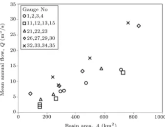
re-gionalized variable is uniformly distributed throughout the basin, indicating a homogeneous basin, where the increase in ow volume is proportional to enlargement of the basin area. If the stationarity hypothesis is valid, ordinary kriging is applicable. This hypothesis can be proved by investigating the relationship between ow and basin area for nested basins, i.e. the basin of one gauge is part of a larger basin contributing to another gauge [2]. However, the study area includes a mixture of nested and non-nested basins; therefore, nested basins are separated and investigated using their ow data and areas. As seen from Figure 2, ow increases with the basin area for nested basins in the region. For the coastal part of the Eastern Black Sea Region, the rainy and humid climate is responsible of abundance water resources in the basins, where both ow and ow depth increase in the downstream direction. Based on the approximate linear relationship between ow and basin area of the nested basins and climate characteristics of the region, ow depth is assumed to be homogenously distributed all over the region and, therefore, ordinary kriging can be applied. On the other hand, being dierent from other meteorological variables such as precipitation, ow depth is related to basin area and represents an area instead of a point. Therefore, the representative value
Figure 2. Relationship between ow and basin area in nested basins.
of the ow depth is allocated on the centroid of the basin [2] instead of the actual observation location, which is the outlet of the basin. Centroids of each basin in the study area are shown in Figure 1.
As geostatistics works generally best when data have a normal distribution, ow data have been checked against normality. The data are found to be normally distributed at signicance level of 0.05. In developing the empirical variogram, only the isotropy case is considered. Because of the limited data, only the omnidirectional variogram is computed, which means in all directions the spatial variabilities are assumed to be identical [25]. Theoretical model tting is carried out using one of the most frequently applied methods, namely, cross-validation approximation. The empirical isotropic variogram and tted model are shown in Fig-ure 3. A Gaussian model is tted and cross-validated with observed data. The validity of Gaussian model is veried using determination coecient (R2), Root
Mean Square Error (RMSE), and mean standardized residual error (MSRE), calculated as:
Figure 3. Experimental variogram of the ow depth with Gaussian model tted.
RMSE = "
1 N
N
X
i=1
(Qesti Qobsi)2
#1=2
; (5)
MSRE = "
1 N
N
X
i=1
(Qesti Qobsi)=i
#
; (6)
where Qest and Qobs represent estimated and observed
ows, N is the number of data, and is the standard deviation of estimation error. The best t of a theoretical model to an empirical variogram is achieved when MSRE approximately equals zero. On the other hand, RMSE is better for the estimation eciency of the extremes [26,27].
Cross validation results of the observed and esti-mated ow depth values for ordinary kriging method are given in Table 2 and Figure 4(a). As seen from Table 2, RMSE value is 185.76 mm for the ow depth data of which minimum, mean, and maximum values are 382.0, 996.3, and 2284.9 mm, respectively.
A previous study [28] has indicated that spatial distribution of precipitation on the coastal part of the Eastern Black Sea Region is not homogenous. Precipitation increases slightly with longitude, which means that the north-eastern part of the region receives greater precipitation than the western part does. Due to the amount of precipitation, ow values of the southern part are greater, i.e. a trend is observed in the ow depth data such that the average varies over the study area. As previously dened, universal kriging can incorporate the eect of the trend. The universal kriging algorithm can produce a trend model by tting a polynomial function to the ow depth data. The locations of ow observation points are plotted on the
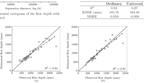
Table 2. Cross validation of ow depth. Ordinary Universal
R2 0.84 0.87
RMSE (mm) 185.76 164.48
MSRE -0.059 -0.009
x y plane and depicted in Figure 5, from which a quadratic trend on the east-west direction and a linear trend on the north-south direction are observed. These trends, represented by a mathematical formula, are removed from the observations and added back before estimations are made. Cross validation results of observed and estimated ow depth values for universal kriging are given in Table 2 and Figure 4(b), after removing trends from the data. As seen from Table 2 and Figure 4, the dierence in calibration between
Figure 5. Trend analysis of ow depth data.
ordinary and universal models is minor; however, universal method seems better based on the R2 (0.87)
and MSRE (-0.009) values.
The kriged maps of ow depth are shown in Figure 6. Streamow maps are similar. Increase in the ow depth from west to east side of the study area is clear in both maps.
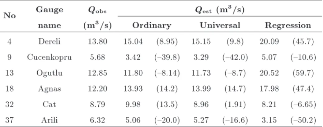
To test the validity of the ow depth map, 6 among 40 ow gauges are randomly chosen. The validation results of randomly chosen gauges are sum-marized in Table 3, where RE shows the relative error in percent, calculated as:
RE = QestQ Qobs
obs 100: (7)
The equivalent ow depths are multiplied by their corresponding areas and ow estimations (Qest) at any
validation points are yielded. In the validation stage, kriging methods are compared with simple regression equation, which is shown in Figure 7. R2of area based
regression equation is 0.70, which is lower than that of kriging methods. Although R2 value can be
statisti-cally accepted, this result conrms that drainage area alone is not adequate to explain regional dierences in
Table 3. Validation results based on the streamow maps and regression.
No Gauge Qobs Qest (m3/s)
name (m3/s) Ordinary Universal Regression 4 Dereli 13.80 15.04 (8.95) 15.15 (9.8) 20.09 (45.7) 9 Cucenkopru 5.68 3.42 ({39.8) 3.29 ({42.0) 5.07 ({10.6) 13 Ogutlu 12.85 11.80 ({8.14) 11.73 ({8.7) 20.52 (59.7) 18 Agnas 12.20 13.93 (14.2) 13.99 (14.7) 17.98 (47.4) 32 Cat 8.79 9.98 (13.5) 8.96 (1.91) 8.21 ({6.65) 37 Arili 6.32 5.06 ({20.0) 5.27 ({16.6) 3.15 ({50.2)
Note: Parentheses represent relative errors (RE%).
Figure 7. Simple regression relationship between ow data and basin area.
annual streamow [29]. In addition, R2 seems to be
partially controlled by the position of greater values (points on upper right position in Figure 7), which indicates an unstable situation [30].
In the validation stage, minimum and maximum relative errors are -39.8 and 14.2 in ordinary, -42.0 and 14.7 in universal, and -50.2 and 59.7 in regression equa-tions. Relative errors are high in low ow estimations; as a comparison criterion, it seems to be meaningless and, therefore, the Absolute Error (AE), which is the dierence between estimation and observation, can be accepted. For the gauge Cucenkopru (No 9), which has the highest RE, AEs are found to be -2.26 and -2.39 m3/s in ordinary and universal models,
respectively. The validation results appear satisfactory in terms of kriging methods.
5. Conclusion
In this study, to determine spatial variation of ow, streamow maps were produced for the coastal part
of the Eastern Black Sea Region, Turkey. The mean annual ow depth was considered as a regionalized variable, thus ordinary and universal kriging methods could be applied.
Mean annual ow depth was obtained using mean annual ow observation, which represents the dierence between annual evaporation and precipitation and provides a measure of the overall water resource for a region. It gives valuable information on the basin under consideration and is useful for comparing water amount in one basin with that in another one. It is used for surface water hydrology and hydrologic design, and characterizes the ow regime in a stream.
In this study, two kriging methods were used. Ordinary kriging is commonly used in practice and has various applications in streamow estimation studies. On the other hand, universal kriging assumes that a trend is available over the area. Universal kriging is also performed when there is spatial variability of the precipitation in the study area.
Kriging methods were compared with simple re-gression based on the relationship between ow data and basin area. From this study, the following conclu-sions can be drawn:
Kriging application of mean annual ow depth provided satisfactory results, meaning that it was useful for ow data at annual time scale;
The performance of kriging models was superior to that of the regression model based on the ow data and basin area relationship. Considering calibration results, universal kriging was better than ordinary kriging, but the dierence was not statistically signicant;
The ow depth map can be a useful tool for ow estimation on ungauged locations in the Eastern Black Sea Region. Promising results of calibration and validation encourage one to suggest this method for other hydrologic applications in dierent regions in Turkey.
Acknowledgements
This study has been supported by the Scientic and Technical Research Council of Turkey, under project number TUBITAK 106M043. The authors would like to thank the anonymous reviewers for their valuable comments and suggestions to improve the quality of the paper.
References
1. Milly, P.C.D. and Dunne, K.A. \Macroscale water
uxes: 1. Quantifying errors in the estimation of basin mean precipitation", Water Resour. Res., 38(10), pp. 1-14 (2002).
2. Huang, W.C. and Yang, F.T. \Streamow estimation
using Kriging", Water Resour. Res., 34(6), pp. 1599-1608 (1998).
3. Rochelle, B.P., Stevens Jr., D.L., and Church, M.R.
\Uncertainty analysis of runo estimates from a runo contour map", Water Resour. Bull., 25, pp. 491-498 (1989).
4. Krug, W.R., Gebert, W.A., Graczyk, D.J., Stevens,
D.L., Rochelle, B.P., and Church, M.R. \Map of mean annual runo for the northeastern, southeastern, and mid-Atlantic United States Water Years 1951-80", U.S. Geological Survey Water Resources Investigations Report, Madison, WI (1990).
5. Bishop, G.D. and Church, M.R. \Automated
ap-proaches for regional runo mapping in the north-eastern United States", J. Hydrol., 138, pp. 361-383 (1992).
6. Merz, R. and Bloschl, G. \Flood frequency
regional-isation { spatial proximity vs. catchment attributes", J. Hydrol., 302, pp. 283-306 (2005).
7. Arnell, N.W. \Grid mapping of river discharge", J. Hydrol., 167, pp. 39-56 (1995).
8. Gottschalk, L. \Correlation and covariance of runo", Stoch. Hydrol. Hydraulics., 7(2), pp. 85-101 (1993).
9. Gottschalk, L. \Interpolation of runo applying
objec-tive methods", Stoch. Hydrol. Hydraulics., 7(4), pp. 269-281 (1993).
10. Sauquet, E., Gottschalk, L., and Leblois, E. \Mapping
average annual runo: A hierarchical approach apply-ing a stochastic interpolation scheme", Hydrol. Sci. J., 45, pp. 799-816 (2000).
11. Sauquet, E. \Mapping mean annual river discharges:
Geostatistical developments for incorporating river network dependencies", J. Hydrol., 331, pp. 300-314 (2006).
12. Sauquet, E., Gottschalk, L., and Krasovskaia, I.
\Es-timating mean monthly runo at ungauged locations: An application to France", Hydrol. Res., 39(5-6), pp. 403-423 (2008).
13. Skoien, J.O., Merz, R., and Bloschl, G. \Top-kriging { geostatistics on stream networks", Hydrol. Earth Syst. Sci., 10, pp. 277-287 (2006).
14. Laaha, G., Skoien, J.O., and Bloschl, G. \Spatial
prediction on river networks: Comparison of top-kriging with regional regression", Hydrol. Process., 28, pp. 315-324 (2014).
15. Archeld, S.A., Pugliese, A., Castellarin, A., Skien,
J.O. and Kiang, J.E. \Topological and canonical krig-ing for design ood prediction in ungauged catchments: an improvement over a traditional regional regression approach?", Hydrol. Earth Syst. Sci., 17, pp. 1575-1588 (2013).
16. Pugliesse, A., Farmer, W.H., Castellarin, A.,
Arch-eld, S.A., and Vogel, R.M. \Regional ow duration curves: Geostatistical techniques versus multivariate regression", Adv. Water Resour., 96, pp. 11-22 (2016).
17. Yan, Z., Xia, J., and Gottschalk, L. \Mapping runo
based on hydro-stochastic approach for the Huaihe River Basin, China", J. Geogr. Sci., 21(3), pp. 441-457 (2011).
18. Kaygusuz, K. and Sari, A. \Renewable energy
po-tential and utilization in Turkey", Energ. Convers. Manag, 44, pp. 459-478 (2003).
19. Eris, E. \Determination of spatial distribution of
precipitation on poorly gauged coastal regions", PhD Thesis, Istanbul Technical University, Institute of Science and Technology (2011).
20. Eris, E. and Agiralioglu, N. \Homogeneity and trend
analysis of hydrometeorological data of the eastern black sea region, Turkey", JWARP, 4, pp. 99-105 (2012).
21. Sima, S. and Tajrishy, M. \Developing water quality
maps of a hyper-saline lake using spatial interpolation methods", Sci. Iran., 22(1), pp. 30-46 (2015).
22. Isaaks, E.H. and Srivastava, R.M., Applied
Geostatis-tics, Oxford University Press, NY (1989).
23. Goovaerts, P., Geostatistics for Natural Resources
Evaluation, Oxford University Press, NY (1997).
24. Journel, A.G. and Huijbregts, Ch.J., Mining Geostatis-tics, The Blackburn Press, NJ (2003).
25. Goovaerts, P. \Geostatistical approaches for
incor-porating elevation into the spatial interpolation of rainfall", J. Hydrol., 228, pp. 113{129 (2000).
26. Gyalistras, D. \Development and validation of a high
resolution monthly gridded temperature and precipita-tion data set for Switzerland (1951{2000)", Clim. Res., 25, pp. 55-83 (2003).
27. Vicente-Serrano, S.M., Saz-Sanchez, M.A. and
Cuadrat, J.M. \Comparative analysis of interpolation methods in the Middle Ebro Valley (Spain): Applica-tion to annual precipitaApplica-tion and temperature", Clim. Res., 24, pp. 161-180 (2003).
28. Eris, E. and Agralioglu, N. \Eect of coastline
cong-uration on precipitation distribution in coastal zones", Hydrol. Process., 23(25), pp. 3610-3618 (2009).
29. Vogel, R.M., Wilson, I. and Daly, C. \Regional
re-gression models of annual streamow for the United States", J. Irrig. Drain. Eng., 125(3), pp. 148-157 (1999).
30. Helsel, D.R. and Hirsch, R.M., Statistical Methods in Water Resources Techniques of Water Resources Investigations, Book 4, chapter A3. U.S. Geological Survey (2002).
Biographies
Ebru Eris, born in 1979 in Izmir, Turkey, received her BSc and MSc degrees from Ege University and PhD degree from Istanbul Technical University. She is currently working as an Assistant Professor in the Department of Civil Engineering, Ege University. She is co-author of 10 international scientic publications and more than 50 international and national proceed-ing papers. She is Vice-President of International Commission of Statistical Hydrology (STAHY) of the International Association of Hydrological Sciences and Secretary of Hidroist (Statistical Hydrology Working Group of the Turkish National Hydrology Commis-sion). She has been involved in national and inter-national activities, including an interinter-national project, bilaterally funded by The Scientic and Technological Research Council of Turkey (TUBITAK) and the Na-tional Research Foundation of Korea (NRF); she was also scientic committee member of the 3rd STAHY
International Workshop on Statistical Methods; orga-nizing Committee member of the 5th EGU Leonardo Conference, Facets of Uncertainty; and a co-convener of IAHS symposia and workshops in the 26th IUGG General Assembly. She worked as a guest researcher at the LEUPHANA, University of Luneburg, Germany, between October 2014 and June 2015.
Necati Agiralioglu was born in 1947. He received his MSc and PhD from Istanbul Technical University (ITU), Turkey. From 1978 to 1979, he was a researcher at the Colorado State University and Mississippi State University. In 1988, he became Professor in the Civil Engineering Department at ITU. He started to serve as a dean of Sakarya University in 1993. Between the years 2003 and 2009, he was chairman of the Hydraulics Department at ITU. In the 5th World Water Forum, he acted as a Programme Committee Co-Chair. Also, he has worked as a board member of Istanbul Water Supply and Sewerage Administration. He is author/coauthor of 9 books and 35 SCI papers, out of more than 140 scientic publications. He has completed various scientic or technical projects and worked as a consultant. Also, he has supervised 13 PhD dissertations and more than 35 MSc theses.