Residential Energy Consumption in
Orange County, NC
Assessing the Impacts of Local Efficiency Programs
by
Jonathan Daniel Linke
A Master’s Project submitted to the faculty of the University of North Carolina at Chapel Hill
in partial fulfillment of the requirements for the degree of Master of Regional Planning in the Department of City and Regional Planning.
Chapel Hill
2011
Approved by:
_________________________ ______________________
Table of Contents
EXECUTIVE SUMMARY ... 1
ACKNOWLEDGMENTS ... 1
INTRODUCTION ... 2
BACKGROUND ... 2
Energy efficiency in the US ... 2
Urban heat islands ... 5
Site design ... 6
Mandatory building codes ... 8
Voluntary building assessments ... 9
Retrofitting existing structures ... 9
Roof albedo ... 10
Tree shading ... 10
POLICY SIMULATION ... 11
STUDY AREA ... 12
Existing local programs ... 13
METHODOLOGY ... 15
Explanatory variables ... 15
DATA DESCRIPTION ... 17
RESULTS/DISCUSSION ... 19
LOCAL PLANNING IMPLICATIONS ... 24
Targeted implementation ... 24
LIMITATIONS ... 34
CONCLUSION ... 34
List of Tables and Figures
TABLES
TABLE 1: Orange County income level proxy ... 16
TABLE 2: RECS 2005 microdata descriptive statistics ... 18
TABLE 3: Orange County parcel data descriptive statistics ... 19
TABLE 4: Linear regression coefficients ... 20
TABLE 5: Heating energy consumption & policy savings ... 23
TABLE 6: Cooling energy consumption & policy savings ... 23
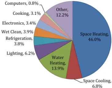
FIGURES FIGURE 1: US residential energy consumption by end use ... 4
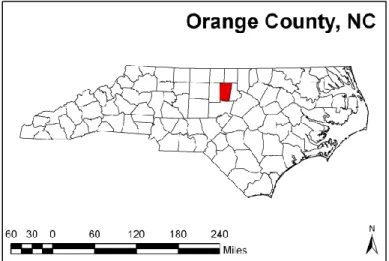
FIGURE 2: Study Area: Orange County, NC ... 13
FIGURE 3: Orange County NDVI map ... 25
FIGURE 4: Selected areas for policy implementation ... 26
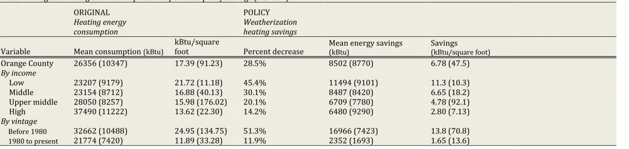
FIGURE 5: Chapel Hill site, NDVI by building vintage ... 27
FIGURE 6: Chapel Hill site, NDVI by household income ... 27
FIGURE 7: Hillsborough site, NDVI by building vintage ... 27
FIGURE 8: Hillsborough site, NDVI by household income ... 27
FIGURE 9: Orange County tree canopy cover map ... 29
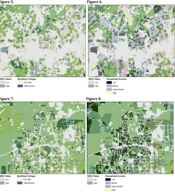
FIGURE 10: Chapel Hill site, canopy cover by building vintage ... 30
FIGURE 11: Chapel Hill site, canopy cover by household income ... 30
FIGURE 12: Hillsborough site, canopy cover by building vintage ... 30
EXECUTIVE SUMMARY
Potential improvements to the energy efficiency of residential buildings present planners and policymakers a number of options for effecting local changes in energy consumption patterns. The possibility of increasing energy efficiency in the US building stock has been explored over the past several decades; however, the geographic scope is often too coarse to account for unique local variables. This paper builds upon past analyses of the
relationship between housing characteristics and residential energy consumption to better understand the energy savings potential of local efficiency programs in Orange County, NC. Two energy models for residential consumption were constructed using Residential Energy Consumption Survey variables that were also available in a county parcel dataset. Three policy interventions were simulated for both heating and cooling energy consumption: (1) weatherization, (2) reflective roofing, and (3) tree shading. Overall, if applied uniformly for the entire county, the policies demonstrate potential to save 29, 13 and 19 percent of
current heating and cooling energy use, respectively. All three interventions prove most effective for low income households, as well as older (pre-1980) as opposed to newer (1980-present) structures. Weatherization improvements demonstrate the highest heating energy savings potentials for the above variables at 45 percent and 51 percent,
respectively. Whereas high income households save 14 percent and new structures see 12 percent savings. Cooling energy policy simulations show a more limited range of energy use reduction (10-23 percent), with low income households and older structures still receiving the highest savings. Resulting savings are comparable to the national, regional, and statewide estimates that appear throughout the literature. Savings estimates provide local policymakers an indication of the effectiveness of potential energy efficiency
programs.
ACKNOWLEDGMENTS
I am grateful for the valuable contributions from Nikhil Kaza that motivated the
INTRODUCTION
Increasing energy efficiency in residential buildings has been identified as a key avenue through which local government can address the consequences of climate change. As climate change becomes increasingly noticeable phenomenon, both public and private sectors devise strategies that help residents mitigate and adapt to the local impacts of projected changes. Through a combination of energy efficiency programs and improved building standards, municipalities are equipped with tools that can generate local changes and help transition towards more sustainable energy consumption patterns.
Planners have argued the need for energy efficient planning over the last several decades (Crandall, 1982; Owens, 1986; Kaiser et al., 1982). Two main concepts underpin their early arguments: 1) planning for less intrinsic need for energy through site design and urban form, and 2) achieving greater efficiency through technological advancement. For the most part, transportation issues have received the bulk of expert attention with respect to the first argument. These days however, land use, site design, and building science garner a greater share of scholarly consideration. The arguments for energy efficient planning persist today as the body of literature addressing the relationship between land use, urban form, climate change, and energy consumption continues to develop (Ruth & Lin, 2006; Ewing & Rong, 2008; Randolph & Masters, 2008; Stone, 2009; Kaza, 2010).
Working with parcel level data, this study presents one methodology for understanding the impacts of local planning initiatives on residential energy consumption. Residential Energy Consumption Survey (RECS) microdata are regressed to construct two models for space heating and air conditioning energy usage in Orange County residential buildings. Parcel data is subsequently adjusted to simulate policy-induced changes in energy consumption. The main findings suggest (1) that weatherization is the most effective mechanism for reducing residential energy consumption, (2) that low-income households experience the greatest benefit from energy efficiency programs, and (3) that older buildings have a much greater potential for energy savings.
BACKGROUND
Energy Efficiency in the US
uncertainty as to whether or not oil is approaching or has reached peak production (Ewing & Rong 2008; Staley, 2008). Concern over high energy prices and dwindling oil reserves are not the only arguments in favor of improving energy efficiency. Recent episodes of social upheaval in fossil fuel exporting nations highlight the unstable political
environments that further complicate the nation’s energy future.
Perhaps the most compelling argument for reducing energy demand is the growing concern over the consequences of climate change. Over the last century, global surface temperatures have increased with a positive linear trend of 1.3 degrees Fahrenheit, although the rate has nearly doubled over the last 50 years (IPCC, 2007). Based on numerous modeling scenarios, the Intergovernmental Panel on Climate Change (IPCC) projects global temperatures to rise throughout the 21st century between 2 and 12 degrees
Fahrenheit (2007). Subsequent sea-level rise and changes in weather patterns, including increased frequency of heat waves and heavy precipitation events, carry similarly
disconcerting implications for much of the world’s population.
Seeking to minimize the negative impacts of a changing climate, the IPCC identifies
numerous strategies for the global community to collectively pursue. Broadly, the building sector is identified as exhibiting the greatest potential for reducing greenhouse gas (GHG) emissions. After reviewing 80 studies, the IPCC found the overall emissions reduction potential for the building sector to be around 29 percent (Levine et al., 2007). Achieving such reductions in emissions through increased energy efficiency can be accomplished with an array of tools, including site design, high-efficiency appliances, reflective building
materials and a more efficient building envelope (IWG, 2000; Levine et al., 2007; Tiller, 2007).
For decades the building sector has accounted for the highest percentage of total energy consumed in the United States. More than industry and transportation, buildings currently account for 41 percent of U.S. energy consumption (EIA, 2009). More specifically, over half of building sector usage is represented by residential consumption, 22 percent of the nation’s total. Finally, the most widespread housing type, single-family detached, which comprises nearly two thirds of the nation’s housing stock, accounts for approximately 80 percent of all residential energy consumption (HUD, 2009; ACEEE, 2011). In the context of climate change and GHG emissions, the residential sector was responsible for 1.2 billion metric tons of CO2 in 2009 and projects to continue to increase through 2030 (EIA, 2009).
Fortunately, the widespread presence residential buildings presents a noteworthy opportunity to U.S. policymakers to effect changes. Experts continue to express their support of efficiency improvements before U.S. legislators, referring to it as a “low-hanging fruit”, our “fifth fuel”, and our cheapest, quickest, cleanest resource (Energy Efficiency in Buildings, 2009). Given the established link between fossil fuel consumption and GHG emissions, the unprecedented amount of current research on reducing energy consumption through increased efficiency is not surprising.
Based on extensive energy modeling and policy research, efficiency improvements in the residential sector present an opportunity to significantly reduce national energy
consumption and simultaneously prevent deleterious GHG emissions. Researchers contend that the potential to reduce residential energy consumption remains high (Tiller, 2007; Brown et al., 2008; Brown et al., 2010). Thus, improving efficiency standards has become the focal point of many local programs aimed at curbing energy consumption, and remains a fundamental mitigation strategy targeting the negative consequences of climate change.
Recent studies examining energy efficiency improvements in the U.S. have found varying levels of achievable efficiency savings. However, it is methodologically problematic to precisely forecast achievable energy consumption savings and GHG emission reductions from efficiency programs due to incredible variation within the building stock (Owens,
Space Heating, 46.0%
Space Cooling, 6.8% Water
Heating, 13.9% Lighting, 6.2%
Refrigeration, 3.8% Wet Clean, 3.9%
Electronics, 3.4% Cooking, 3.1% Computers, 0.8%
Other, 12.2%
U.S. Residential Sector Energy Consumption
by End Use 2010
(total Btu)
1986). Nevertheless, researchers at institutions such as Oak Ridge National Laboratory (ORNL) and the Lawrence Berkeley National Laboratory (LBNL), among others, have been able to roughly quantify potential savings through the use of modeling programs and energy use projections (IWG, 2000; GDS Associates, 2006; Brown et al., 2008; Brown et al. 2010). These studies indicate residential energy savings between 2 and 33 percent
depending on assumptions concerning technical feasibility and aggressiveness of policy implementation. The geographic scope varies across studies as they analyze national, regional, and state-level energy consumption.
Estimates of energy savings from efficiency improvements establish a foundation for further evaluation and can guide policy decisions which increase the capacity of local governments to plan for energy efficiency. North Carolina currently has the 10th highest
energy consuming residential sector in the nation, using 715 trillion Btu in 2008 (EIA, 2010a). Studies specific to North Carolina find that residential space heating and space cooling exhibit potential for efficiency improvements to reduce energy consumption (Hadley, 2003; Tiller, 2007). This is an important finding because taken collectively, space conditioning accounts for over half of residential building energy consumption (EIA, 2010b). Using econometric models to derive energy savings estimates, these studies consider a range of economic and technical factors including cost, consumer preference, product efficiencies, life cycle cost, fuels used, etc. to iteratively model efficiency potentials for North Carolina. Brown et al. (2010) summarize the savings reported in these and
related studies to range from 8 to 27 percent for the residential sector, mostly attributed to reductions in electricity consumption. Additionally, they refine their scope to consider four key policy options: building code stringency, improved appliance standards, expanding the Department of Energy (DOE) Weatherization Assistance Program (WAP), and retrofit incentives, thereby narrowing savings projections to 10 to 16 percent.
Urban heat islands
The connection between land use, climate change, and energy consumption has received significant attention in recent years (IPCC, 2007; Stone, 2009). The NC State Climate Office contends that while no significant trend in annual temperature anomaly has been observed for the state over the 20th century, warming trends are becoming more noticeable in the
state’s urbanized areas. Temperature records demonstrate that these trends are not paralleled in surrounding rural areas. As a result, the trends are generally attributed to conversion of vegetated land for development. This phenomenon is commonly referred to as the heat island effect. In 2002, Henley revisited a heat island study done in Chapel Hill in 1969 to investigate its morphology over time. She collected field data from points
throughout Chapel Hill to analyze urban heat island (UHI) formation and shift between 1969 and 2001. Her research indicates a spatial correlation between heat island
Heat islands are formed when vegetated land is replaced with impervious surfaces that exhibit relatively low reflectivity to solar radiation. Supporting Henley’s findings, Stone (2006, 2009) argues that sustained urbanization is currently threatening to hasten and intensify local microclimate change, thus contributing to UHI formation. As a result of land conversion, the natural cooling effects of evaporation and evapotranspiration are lost, while at the same time greater amounts of thermal energy are absorbed raising both surface and ambient air temperatures (Sailor, 2007; Gartland, 2008). The configuration of urban surfaces further complicates atmospheric mixing and traps excess heat energy near ground level (Henley, 2002). Anthropogenic waste heat from automobiles, industrial processes and heating and cooling systems further contributes to UHI formation. The resulting temperature difference between urban and rural land can be as great as 15 degrees Fahrenheit and can significantly increase cooling energy demand (Ewing & Rong, 2008; Gartland, 2008). Conversely, heat islands in can also reduce winter heating demand; although increases in cooling energy demand generally far outweigh these perceived benefits.
The consequences of UHI formation elicit attention from the planning field. Heat island-induced increases in ambient summertime temperatures result in greater accumulation of cooling degree days (CDD). Subsequently, air conditioning demand increases to
compensate for the larger temperature differential. As a result, the UHI can significantly impact citywide energy consumption (Stone, 2006; Sailor, 2007; Ewing & Rong, 2008). A shift in demand from space heating towards space cooling signifies a shift in energy source as well. In 2000, 37 percent of residential space heating in North Carolina was derived from natural gas whereas only 11 percent came from electricity (Hadley, 2003). On the other hand, space cooling is entirely powered by electricity, which in 2009 was responsible for 94 percent of the nation’s coal consumption and has more serious implications for GHG emissions (EIA, 2009). Finally, higher ambient temperatures can be fatal to sensitive
populations and raise concerns over air quality as higher temperatures play a major role in the formation of ozone (Stone, 2006).
Site design
Ian McHarg’s seminal work Design with Nature was the first to systematically illustrate the importance of planning in harmony with existing natural conditions (climatic, topographic, hydrologic, etc.). David Crandall (1982) argues that technological advancements in building systems and materials have speciously lured the building community away from McHarg’s principles. Today however, his principles are reemerging as connections between
environmentally sensitive design and energy savings continue to be drawn. Consequently, building rating systems including the United States Green Building Council (USGBC)
Leadership in Energy and Environmental Design (LEED) and the ENERGY STAR program, a collaborative effort between the DOE and EPA, are stressing environmental consideration in design parameters.
For one example, taking advantage of solar resources can minimize building energy use. Furthermore, builders can utilize knowledge of solar angles to carefully locate features such as window overhangs as a means of managing seasonal solar access and in turn reducing total energy demand in buildings (Marsh, 2005; Randolph & Masters, 2008). Familiarity with the interaction between onsite wind speeds and topography also carry significant heating and cooling implications for buildings (Crandall, 1982; Marsh, 2005). Building orientation is equally important when planning energy efficient site designs. Orienting buildings along an east-west axis limits exposure to incoming solar radiation in summer months and allows for solar heat gain in winter months. Conversely, buildings oriented along a north-south axis experience sustained periods of horizontal solar
radiation in the morning and afternoon, making shading from trees or overhangs much less feasible and heat gain, therefore, harder to mitigate (Randolph & Masters, 2008).
Mandatory building codes
Building codes adopt some of the conceptual framework behind site design practices to establish minimum engineering specifications for new construction and additions or renovations. Energy conservation codes are a common component of statewide building codes that regulate energy related building systems. Energy efficiency requirements address thermal resistance (R-factor), thermal transmittance (U-factor), fenestration, ventilation and so on (Building Codes Assistance Project, 2011). Structures built to meet up-to-date building codes benefit from availability of state-of-the-art technologies and building practices, enabling them to realize efficiencies unparalleled by retrofit programs.
In many analyses, the year 1980 is used as a transitional building vintage to differentiate between new and old structures. It represents a point in time when most states had adopted a preliminary version of building code that incorporated insulation, fenestration, and HVAC systems requirements (Akbari, Konopacki, & Pomerantz, 1999; Randolph & Masters, 2008; Aroonruengsawat, Auffhammer, & Sanstad, 2009; Chong, 2010). North Carolina’s amendments to the Southern Building Code Congress Standard Building Code in 1978 were the first to address insulation and double paned windows, and therefore
coincide well with the 1980 threshold (Buildings Codes Assistance Project, 2011). Additionally, a study of North Carolina households by Kaiser, Marden and Burby (1982) found dramatic increases in energy efficient equipment and building practices between 1960 and 1978.
The DOE states that more stringent building codes have largely been responsible for 9 percent decrease in energy intensity on a per household basis from 1985 to 2004 (DOE, 2008). In light of these advances and pervasive adoption of codes nationwide, researchers continue to explore building code effectiveness at reducing energy consumption. Recent studies have investigated time series of residential energy bills to clarify the relationship between code adoption and energy use (Aroonruengsawat, Auffhammer, & Sanstad, 2009; Kotchen and Jacobsen, 2009; Chong, 2010). While two of the above studies find building code to reduce annual residential energy consumption by 3 to 6 percent, Chong (2010) concludes that a lack of code enforcement and implementation can severely undermine the energy efficiency claims of new and improved code. His findings echo a general skepticism toward building code enforcement and compliance (Building Codes Assistance Project, 2011).
stringency above the 2006 IECC with notable improvements to duct insulation and sealing, envelope specifications and lighting efficiency (Pacific Northwest National Laboratory, 2009; ACEEE, 2010). The decision to adopt a new code of such stringency demonstrates a statewide effort to reduce energy consumption.
Voluntary building assessments and labeling
The movement toward more energy efficient residential buildings is reflected in the
growing prevalence of voluntary green building certification programs and rating systems. These programs are considered produce “above code” buildings that are more efficient than baseline requirements established in codes. Researchers cite issues such as higher energy costs, goodwill benefits, higher awareness of global climate change, and general tenant demand for the recent uptrend in above code construction (Nelson, 2007). As a result, rating and certification programs such as LEED and the U.S. EPA’s ENERGY STAR program are gradually increasing the market penetration of energy efficient residences.
Through a comprehensive approach to improving whole-building efficiency, these programs report energy savings of nearly 30 percent compared to baseline estimates (Nelson, 2007). Additionally, each program requires third party verification of building system performance, which eliminates non-compliance issues raised by Chong (2010). While LEED certification has largely been utilized for multi-family housing, office, and retail buildings, ENERGY STAR continues to make its greatest impact in the residential sector. Of the nearly 24,000 ENERGY STAR certified homes in North Carolina as of April 2011, 7,300 were built in 2010 alone, representing roughly 30 percent (U.S. EPA & U.S. DOE, 2011). This highlights the growing trend in the residential building community of providing more energy-efficient structures.
Retrofitting existing structures
Retrofitting existing buildings is often cited as the most effective way to reduce residential sector energy consumption (Levine et al., 2007, Energy Efficiency in Buildings, 2009). While new construction constitutes a valuable resource for reducing residential energy use, a majority of buildings responsible for residential energy consumption have already been built.
Since its inception in 1976, the DOE’s Weatherization Assistance Program (WAP) has found success improving the energy efficiency of low-income residences, now reporting average annual savings on energy bills around $437 USD (2010) per household. Initially, the term weatherization referred to simple home improvements that increased building efficiencies such as weather-stripping doors and sealing cracks in the building envelope. The practice has since evolved to encompass a more comprehensive understanding of building
Eligibility for WAP is restricted, however, and is contingent upon several factors:
household size, composition and income level. Further, availability of assistance is limited to low-income households and certain excepted cases. The DOE defines low-income households (size dependent) as earning below 200 percent of the poverty level.
Under the more modern framework of weatherization practice there have been numerous metaevaluations of state-level WAP assessments conducted through ORNL and DOE
partnerships. WAP has been documented to be more effective in colder climates; therefore natural gas for space heating tends to be the dependent variable in question for most evaluations. The most recent studies present a nationwide average of 23 percent savings per household for all natural gas end uses and 32 percent energy savings on natural gas consumption for space heating alone (Schweitzer, 2005). Schweitzer also evaluates WAP effectiveness on non-heating uses, finding savings between 5 and 8 percent. Non-heating estimates are mostly from cooling energy reductions, though admittedly, savings are drawn from a much smaller sample of studies. Additionally, while not specifically addressing the effectiveness of the federal program, Tiller et al. (2007) indicate that weatherization
measures contribute approximately 60 percent of their projected energy savings estimates.
Increase roof albedo
Traditional roofing materials can reach temperatures as high as 185˚F in summer months (EPA, 2008). Since heat flow into a building is largely a function of external temperature (as well as interior insulation), ambient temperatures above roofs can impact indoor comfort level and therefore the energy use of a home (Akbari, Gartland, & Konopacki, 1998). Additionally, R-values of insulation tend to decrease as temperatures increase, permitting greater amounts of inward heat flow (Berdahl & Bretz, 1997). To reduce energy demand in summer months, researchers analyze the properties of roofing products to find the best ways to establish “cool roofs”. They focus on two main properties of roof materials, solar reflectance or albedo and thermal emittance. Increases to albedo and thermal emittance limit the amount of heat transferred to a home. As a result, cool roofs with high albedo and thermal emittance will only reach temperatures around 120˚F as compared to the 185˚F mentioned above (EPA, 2008).
Tree shading
While all types of vegetation have the potential to reduce buildings energy demand, shade trees are best suited to provide energy saving benefits. For instance, Marsh (2005) suggests that in summer months, a multi-layered tree canopy can block up to 80 percent of incoming solar radiation. Donovan and Butry (2009) found strategically placed shade trees to
throughout the literature (Randolph & Masters, 2008; Sailor, 1998; Marsh, 2005; Gartland, 2008).
POLICY SIMULATION
Orange County parcel data was manipulated to simulate potential energy efficiency policies and programs. The following descriptions provide rationale for the data adjustments that were used in the energy modeling process:
Albedo (CDD reduction)
Most recent studies considering the energy reduction potential of cool roofs report findings in percent cooling energy savings, ranging from 2 to 69 percent (Gartland, 2008). However, in order to model savings using building-specific data in Orange County, an estimated reduction in CDD was needed to regress cooling energy consumption. A selection of cool roof studies provides average air temperature reductions in their results (Akbari,
Konopacki, & Pomerantz, 1999; Gartland, 2008). Using findings from studies conducted in Climate Zone 41, CDD for the Northern Piedmont climate division of North Carolina were
collected and adjusted based on perceived temperature reductions (2.1˚F) from the literature. CDD adjustment was performed for months that have an historical average temperature greater than 65˚F (May-September). To calculate CDD reductions,
temperature reductions taken from past studies were multiplied by the number of days in each applicable month; these values were then summed and subtracted from the annual average CDD recorded for the area.
The Mitigation Impact Screening Tool (MIST), developed by Sailor and Dietsch (2007), provides an excellent mechanism for cross-referencing these estimates. Based on a
combination of internally calibrated building prototypes2 and user-defined inputs such as
local CDD, HDD, population and average temperature, MIST creates a table of possible outcomes of a specified mitigation technique. The tool was used to verify the CDD adjustment process used in this report. Both scenarios assume an increase in albedo of approximately 0.25. Orange County albedo values were assumed to resemble those
observed by Akbari, Konopacki, and Pomerantz (1999) in Atlanta residential buildings, an assumption they apply to the entire South Census region in their evaluation.
Tree shading (CDD reduction)
Employing a nearly identical approach, the effects of shade trees are modeled using CDD reduction estimates. Past studies analyzing the cooling energy savings of tree shading report air temperature reductions between 2-6˚F (Kurn et al., 1994; Gartland, 2008). Based
1 As used by the EIA, Zone 4 areas exhibit less than 4000 HDD and less than 2000 CDD 2 Using DOE-2 building energy analysis software
on interpretations of existing tree canopy cover in the county, more conservative reduction estimates were considered in determining CDD reductions for shading programs. Aerial imagery of Orange County shows substantial existing tree cover. To account for this observation, the model was run using a more conservative estimate (3˚F) of air temperature reduction as a result of tree shading.
Weatherization (building age adjustment)
Home weatherization represents another effective way for communities to reduce energy consumption for space conditioning. This report simulates several scenarios of
weatherization in Orange County. Attribute data from the Orange County GIS parcel files were somewhat limited when compared to the information produced by the RECS public use microdataset. Therefore, building vintage was used as a proxy to demonstrate the effect of home weatherization. Several scenarios were run that considered varying
implementation strategies. Simulations of targeted interventions sought first to
demonstrate weatherization initiatives based on income level, modeling each individually. Two final iterations were run to assess the effects of weatherization based on building vintage, separately modeling structures built before 1980 and after 1980 to simulate bringing a house “up to code”.
To reflect the magnitude of policy decisions, year built data was designated as a proxy indicator of the weatherization quality of a structure. If a particular income level, or building vintage was eligible for a program, housing age was updated to demonstrate the effects weatherization on energy use. For example, if a home built in 1948 was weatherized as a result of a given program, the year built was moved from the 1940 to 1949 vintage range to the 2000+ range, operating under the assumption that weatherizing a house makes it compliant with current building code standards.
STUDY AREA
Existing local programs
To estimate the potential energy savings that Orange County can achieve based on the strategies described above, a review of existing policies and programs enables a better understanding of the local situation. The Database of State Incentives for Renewables & Efficiency (DSIRE) provides a comprehensive list of existing energy programs available in North Carolina. Incentives include loan programs with favorable terms, efficient equipment rebates, utility rate discounts, and a sales tax holiday for energy efficient appliances. In North Carolina, utility companies rather than local governments administer energy efficiency programs under the oversight of the NC Utilities Commission (ACEEE, 2010). Therefore, Duke/Progress Energy and Piedmont Electric are responsible for the majority of efficiency programs in the state. As an example, Piedmont Electric offers loans up to
$10,000 with repayment period of up to seven years at an interest rate of 5 percent. Loans apply to efficiency improvements to central air conditioners, insulation, windows, doors, and heat pumps. Since studies have not yet analyzed the effectiveness of these programs, it is difficult to infer their capacity to reduce statewide residential energy consumption.
Though local government-initiated incentive programs exist, they are limited. This is not surprising as rebates and tax relief are less financially feasible at the local level. On the other hand, municipalities have the ability to affect energy efficiency from a land use policy perspective. A review of energy-related policies in Carrboro, Chapel Hill, and Hillsborough indicates that while energy efficiency has received more recognition in recent years, room remains for program expansion.
Chapel Hill easily demonstrates the greatest commitment to energy efficiency, maintaining multiple policies and programs addressing the issue. Chapel Hill qualifies as a Sierra Club
“Cool City” and is a part of the Cities for Local Climate Protection Campaign (jointly with Orange County and Carrboro). Additionally, Chapel Hill committed to a 60 percent reduction in carbon emissions by 2050 as part of the Community Carbon Reduction Project; the first U.S. municipality to make such a commitment. Participation in these programs exemplifies the town’s commitment to a sustainable future. Commitment to improving residential energy efficiency, however, is most directly demonstrated by the WISE Homes & Buildings Program, which was recently funded by the DOE using American Recovery and Reinvestment Act (ARRA) grant money. This program is intended to
supplement homeowner expenses for efficiency improvements with maximum grants of $5,000, and funds activities comparable to those considered under DOE’s WAP. Contrasting WAP, however, eligibility for WISE is not selective. Unfortunately, grant funding is a finite and relatively unstable form of financial assistance.
Chapel Hill maintains various other initiatives that increase residential building efficiency. Perhaps most importantly, the town leads by example. In 2004 Chapel Hill adopted a municipal green building ordinance that mandates LEED certification of any new or renovated municipal building. In 2003 citizens voted in support of a local Energy Bank which allocates funds for energy efficient improvements to public buildings. Currently, the town maintains a policy promoting green building development—requesting that
developers “demonstrate site planning, landscaping, and structure design which maximize the potential for energy conservation … by reducing the demand for artificial heating, cooling, ventilation, and lighting, and facilitating the use of solar and other energy resources” (Town of Chapel Hill, 2007). Special or conditional use permit approval is therefore contingent upon consideration of such features. To incentivize this requirement, the town passed a resolution to expedite permit processing for projects seeking LEED Silver certification, or comparable energy efficient design. It will be interesting to monitor how developers respond to this provision following the adoption of the updated state building code, which contains 30 percent more stringent energy efficiency requirements than the current code. Finally, Chapel Hill’s Land Use Management Ordinance (LUMO) contains an extensive tree protection provision that specifies measures to preserve tree cover during site design and project development.
Other jurisdictions in Orange County demonstrate a lesser commitment to energy
efficiency when compared to Chapel Hill. Still, a few provisions are worth noting. Through the same DOE grant mentioned for Chapel Hill, the town of Carrboro initiated an Energy Efficiency Revolving Loan Fund to incentivize efficiency improvements for small
developers to consult during design and planning phases. Finally, Hillsborough has recently led by example, undergoing an Energy and Greening Audit of municipal facilities over the last several years. All three incorporated municipalities received Level 1 ratings as part of the North Carolina League of Municipalities Green Challenge.
Together, awareness of climate change and higher energy prices has played a significant role in the promulgation of local, energy efficient building initiatives. Local governments are beginning to embrace energy efficiency as an asset to their respective communities. Therefore, policies such as those outlined above are not uncommon and will continue to gain acceptance as their effectiveness becomes better understood. The remainder of this report estimates the potential effects of additional policies that could be pursued by Orange County governments.
METHODOLOGY
Of the energy efficiency studies motivating this report, nearly all incorporate methods that aggregate and/or extrapolate state and regional level energy use data. Therefore, energy savings potential of efficiency programs has historically been derived at relatively coarse geographies. Such estimations are helpful in determining regions that exhibit higher potential for improvement; though at the same time, they highlight the need for place-specific studies to refine the scope of their inquiry.
One of the most frequent criticisms of energy efficiency studies is that generalized estimates fail to account for place-specific climatic, building, and regulatory conditions. This paper on the other hand, seeks to overcome such indistinct geographic shortcomings by utilizing a more nuanced approach and analyzing variables such as energy use and housing characteristics in Orange County. Additionally, this investigation incorporates a spatially detailed component to the energy savings assessment, by mapping building parcels to understand housing vintage distribution and vegetative coverage using geographic information systems. Furthermore, adding a spatially explicit element to the analysis enables policymakers to geographically prioritize energy efficiency policies and programs, allowing a more directed allocation of resources.
Explanatory variables
activity, and building factors. As their study focuses on commercial buildings, principal activity may have less of a place for residential considerations; however, household size and ownership status are conceivably designated under this heading. For the most part, analysis of housing characteristics has identified the following variables as effective predictors of residential energy consumption: housing area, housing type, year built, climatic conditions (CDD and HDD), household size, annual household income, and average energy price.
To construct a site-specific model of residential energy use for Orange County, regression variables were selected to coincide with available parcel data. Therefore, the following RECS variables were regressed: housing area, annual household income, average energy price, HDD, CDD, and year built. RECS 2005 microdata were regressed against specific residential energy uses to obtain coefficients for developing the local energy model. Annual household income required the use of a proxy variable as it is not included in the parcel dataset. Therefore, total property value was utilized to approximate annual household income. These data were then separated into four income levels with breaks shown in Table 1. Finally, dummy variables were assigned to both year built and income ranges.
Table 1.
Property value* thresholds for income level proxies
Income Level Property Value
Low <150k
Middle 150-300k
Upper Middle 300-500k
High 500k+
*2010 Orange County parcel data
Separate regressions were run for space heating and air conditioning, two of the dominant energy uses in residential buildings. Regressions incorporate energy usage from the
following fuels: electricity, natural gas, fuel oil, and liquefied petroleum gases, as they account for 98 percent of residential energy consumption (EIA, 2010a)3. Electricity
represents the only fuel reported for space cooling in the RECS data. British thermal unit (Btu) usage for all fuel types was aggregated to determine the total energy used for space heating. Coefficients were then used to construct separate energy models to simulate energy consumption in Orange County residences. Finally, data were manipulated to demonstrate the effect of policy interventions on residential energy use.
DATA DESCRIPTION
RECS 2005 microdata
Two primary datasets form the basis of the ensuing policy-based energy modeling. The underlying regression equation and energy use coefficients are derived from 2005 RECS public use microdataset published by the U.S. Energy Information Administration (EIA). The microdata provide survey responses from 4,382 randomly sampled households, which then use area-probability to estimate the national data in RECS datasets (EIA, 2009). Table 2 provides summary statistics for the microdata used in regression.
Orange County parcel data
Comprising the local dataset, parcel data for Orange County is supplemented with area averages of CDD and HDD, and average North Carolina energy pricing data from 2008. University of North Carolina Libraries, through a data sharing partnership with local municipalities, provided parcel data, which is current through January of 2010. CDD and HDD data were obtained through the State Climate Office of North Carolina NC CRONOS database, and use 65˚F as the baseline temperature. Orange County falls within the
Northern Piedmont region of North Carolina, therefore this report includes average annual CDD and HDD totals from this region between 1895 and 2010. Finally, the EIA provides a State Energy Profile for North Carolina, which gives statewide energy pricing figures in dollars per million Btu.
The most recent parcel data available for Orange County are detailed, yet imperfect.
Table 2.
RECS 2005 microdata descriptive statistics
Housing Variable Mean Std. dev. 25% Median 75%
Heating energy (kBtu) 41585 40585 8820 31134 63533
Cooling energy (kBtu) 7238 8762 986 4323 10376
Total heating area (sq ft) 1602 1158 831 1312 2072
Total cooling area (sq ft) 1338 1531 221 832 1940
Heating degree days (˚F) 4311 2181 2382 4639 5927
Cooling degree days (˚F) 1486 966 835 1282 1858
Average price (per MBtu) 20.58 7.06 15.63 19.48 23.99
Count Percentage
Year built
Before 1940 640 15
1940-49 281 6
1950-59 514 12
1960-69 489 11
1970-79 751 17
1980-89 724 17
1990-99 653 15
2000+ 330 8
Annual household income
<20k 1143 26
20-40k 1133 26
40-70k 1039 24
70k+ 1067 24
Table 3.
Orange County 2010 parcel data descriptive statistics
Variable Mean Std. dev. 25% Median 75%
Total conditioned area 1810 919 1176 1568 2208
By income
Low 1161 365 945 1088 1296
Middle 1522 501 1204 1441 1759
Upper middle 2163 753 1680 2103 2551
High 3132 1211 2353 2992 3672
By vintage
Pre-1980 1555 866 1048 1344 1798
1980 - present 2004 938 1308 1784 2486
Property value ($) 303316 227097 151900 244500 387300
Count Percent
Year built
Before 1940 2683 7
1940-49 1476 4
1950-59 2916 7
1960-69 4508 11
1970-79 5247 13
1980-89 7480 19
1990-99 8121 20
2000+ 7580 19
Mean building age 1978
Median building age 1984
Property value (income proxy)
<150k 9733 24
150-300k 14915 37
300-500k 9846 25
500k+ 5515 14
Average price ($ per MBtu)* 24.99
Total Observations** 40011
*2008 SEDS, EIA
**Excludes parcels not reporting year built data, parcels over 10,000 square feet, and property values over $5 million
RESULTS/DISCUSSION
The effects of three energy efficiency policies were simulated for Orange County residential housing stock using derived energy models. Table 4 provides coefficient results for space heating and air conditioning regressions of RECS microdata. Analyzing coefficient
magnitudes allows us to better understand the overall effect of explanatory variables on residential energy consumption. It is straightforward that house area is positively
energy consumption. The same concept holds true for HDD and CDD. A one degree day increase in HDD has a greater impact on energy use than a one degree day increase in CDD, although both represent relatively marginal changes. The concern is that a warming
climate will result in sustained increases in CDD and will therefore become less marginal over time.
Table 4.
Linear regression coefficients (RECS 2005)
Heating Cooling
Household Variables Coefficient p-Value Coefficient p-Value
Constant 19699.9 <0.001 -5373.8 <0.001
Adjusted R2 0.4966 0.5792
House size
Heated square feet 6.0 <0.001 NA NA
Air conditioned square feet NA NA 2.2 <0.001
Year built
Before 1940 31496.4 <0.001 304.6 0.368
1940-1949 20420.4 <0.001 520.2 0.218
1950-1959* 18445.4 <0.001 --- ---
1960-1969 15294.1 <0.001 94.7 0.792
1970-1979 9135.8 <0.001 548.9 0.092
1980-1989 4033.4 0.036 1147.1 0.001
1990-1999 2998.4 0.124 1416.4 <0.001
2000+* --- --- 1652.4 <0.001
Household income
20-40k 779.7 0.521 768.9 0.001
40-70k 3597.4 0.005 1136.7 <0.001
70k+ 7431.9 <0.001 1518.8 <0.001
Average energy price ($ per kBtu) -1622091.0 <0.001 218449.2 <0.001
Heating degree days 7.0 <0.001 NA NA
Cooling degree days NA NA 5.2 <0.001
*Notes: Year built categories are contrasted against the '2000+' category for heating and '1950-1959' for cooling. Vintages were specifically chosen as the contrast category because they demonstrated the lowest energy use estimates for the particular category. Household income categories are contrasted against the 'less than 20 K' income category.
NA = Not Applicable
the Orange County data indicate that the mean square footage of residences has increased from around 1500 to 2000 since 1980. While this partially explains coefficient increases with building age for cooling energy, one might expect the increases to be paralleled by space heating consumption. Instead, space heating coefficients decrease with age. This provides indication that more stringent building codes and energy efficient building materials are producing the desired reductions in household heating energy consumption. Finally, year built coefficients were statistically insignificant for structures built before 1980 in the cooling energy regression equation. Since year built was the explanatory proxy manipulated to simulate weatherization efforts, models were not run to estimate the
effects of weatherization on cooling energy consumption. Increased housing area, central cooling system prevalence in newer residences, and behavioral changes are likely to decrease the significance of the year built coefficient in the cooling equation.
Instead, savings rates from previous WAP evaluations can be applied to baseline cooling energy estimates to give a rough indication of achievable savings from weatherization. There is relatively little validity to these predictions; however, past studies suggest that weatherization efforts can save between 5 and 8 percent of household cooling energy consumption (Schweitzer, 2005). These estimates do become more significant when considering the additive benefits of weatherization and other cooling energy efficiency policies.
While negative coefficients for heating energy pricing demonstrate an expected effect on energy consumption, the cooling energy regression produces a positive coefficient. Logically, the more expensive it becomes to consume energy for either end use, the less a household will consume. Regression results indicate this to be true for heating energy, though not for cooling. It has been suggested in the literature that households are becoming more energy dependent, therefore making energy more price inelastic (Kaza, 2010). While this does not necessarily explain the positive coefficient, it should be noted that in comparison to the magnitude of the heating energy price coefficient, cooling is much less significant. The implication here is that while increasing energy price will theoretically result in reduced space heating energy consumption, it does relatively little to affect
cooling energy demand.
Tables 5 and 6 show modeled baseline heating and cooling energy consumption estimates both by income level and by housing vintage. They also demonstrate potential energy savings estimates associated with each policy intervention. Overall, if weatherization policy was implemented uniformly, the county could reduce total space heating energy
efficiency studies consulted during the literature review. On the other hand, cooling energy savings are slightly lower than previous estimates. This is likely attributable to two factors: (1) that Orange County has substantial tree cover to begin with so conservative estimates of temperature reduction from shade were used, and (2) albedo increases used
conservative assumptions of existing roof albedo, and therefore did not present as great a change as previous studies.
Table 5. Original heating Btu consumption and potential policy savings (std. dev.)
ORIGINAL POLICY
Heating energy consumption Weatherization heating savings
Variable Mean consumption (kBtu)
kBtu/square
foot Percent decrease Mean energy savings (kBtu) Savings (kBtu/square foot)
Orange County 26356 (10347) 17.39 (91.23) 28.5% 8502 (8770) 6.78 (47.5)
By income
Low 23207 (9179) 21.72 (11.18) 45.4% 11494 (9101) 11.3 (10.3)
Middle 23154 (8712) 16.88 (40.13) 30.1% 8487 (8420) 6.65 (18.2)
Upper middle 28050 (8257) 15.98 (176.02) 20.1% 6709 (7780) 4.78 (92.1)
High 37490 (11222) 13.62 (22.30) 14.2% 6480 (9290) 2.80 (7.13)
By vintage
Before 1980 32662 (10488) 24.95 (134.75) 51.3% 16966 (7423) 13.8 (70.8)
1980 to present 21774 (7420) 11.89 (33.28) 11.9% 2352 (1693) 1.65 (13.6)
Table 6. Original cooling Btu consumption and potential policy savings (std. dev.)
ORIGINAL POLICY POLICY
Cooling energy consumption Shade cooling savings Albedo cooling savings
Variable Mean consumption (kBtu)
kBtu/square
foot Percent decrease Savings (kBtu/square foot) Percent decrease Savings (kBtu/square foot)
Orange County 12999 (2599) 8.55 (51.4) 19.2% 1.74 (13.57) 13.4% 1.21 (9.49)
By income
Low 9733 (10580) 9.69 (2.16) 23.0% 2.26 (.740) 16.1% 1.58 (0.478)
Middle 14915 (12340) 9.07 (38.9) 19.7% 1.84 (10.1) 13.8% 1.29 (7.04)
Upper middle 9846 (1834) 8.03 (91.35) 17.2% 1.50 (24.3) 12.0% 1.05 (17.0)
High 5548 (16817) 6.11 (13.4) 14.7% 0.95 (3.22) 10.3% 0.666 (2.25)
By vintage
Before 1980 11659 (2191) 9.09 (69.84) 21.2% 2.03 (18.6) 14.8% 1.42 (13.0)
1980 to present 13974 (2432) 8.17 (31.9) 17.7% 1.53 (8.23) 12.4% 1.07 (5.75)
LOCAL PLANNING IMPLICATIONS
The savings estimates modeled above present Orange County policymakers with several options for reducing residential energy consumption. As noted earlier, space heating and cooling constitute a majority of residential energy consumption.
Therefore, focused policy efforts to bring about changes in these end uses should be a priority for local governments. Energy efficiency improvements have been
demonstrated to bring significant savings to specific populations; the ensuing challenge for local governments is to devise a strategy that enables public adoption of such improvements.
Targeted Implementation
Municipalities can begin by targeting those properties that demonstrate the greatest energy savings potential. Simply mapping parcel data based on household income or year built attributes provides guidance for targeted weatherization programs. On the other hand, finding parcels that would benefit the most from cooling energy efficiency programs is not as simple.
Remotely sensed imagery can be processed and imported into ArcGIS to assist in targeting program implementation. Policymakers can utilize this data to create prioritization schedules to systematically allocate resources by identifying
appropriate parcels. One example of useful satellite data, NDVI is used to measure the density of vegetation in a given area. NDVI measurements show the relationship between reflected visible and near-infrared radiation. Greener, denser land cover absorbs visible radiation and reflects a larger portion of near-infrared radiation. Therefore, areas with denser vegetative land cover produce higher NDVI values. (National Aeronautics and Space Administration, 2011)
Resulting raster data layers can be used to visually determine areas of importance. From there, the user can transparently overlay the NDVI layer atop symbolized parcel and building footprint data layers to determine specific parcels with low NDVI values. Tree planting and other vegetative screening policies can then be strategically implemented to increase vegetative cover, and therefore realize CDD reductions modeled in this report. Figures 5 through 8 demonstrate how this
process might be undertaken in two sample areas in the County: (1) a neighborhood in west Chapel Hill, and (2) a neighborhood adjacent to downtown Hillsborough.
Figure 5. Figure 6.
Figure 7. Figure 8.
Tree canopy coverage data layers provide a second, more direct, mechanism for informing strategic investments. The United States Geological Survey (USGS) Multi-Resolution Land Characteristics Consortium (MRLC) provides a national dataset of percent canopy coverage. Their most recent product uses 2001 data. Since tree canopy cover has certainly changed over the last decade, directed outreach cannot be accurately recommended using this data. Though again, the concept remains the same. In a sense, tree canopy coverage enables an even more refined approach to reduce cooling energy consumption. As Donovan and Butry (2009) found in their investigation of electricity savings from tree shade, the spatial arrangement of trees with regard to building orientation and sun azimuth results in significantly different realized energy savings. Planners can therefore spatially analyze building
orientation and canopy coverage to target implementation any particular household or housing attribute (i.e. income or building vintage). Figure 9 shows high, medium and low canopy cover percentages indicating general areas where greater tree cover would prove beneficial. Not surprisingly, canopy coverage is the least extensive in areas in closest proximity to town centers.
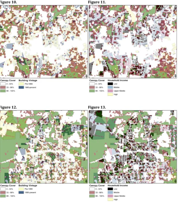
Figure 10. Figure 11.
Figure 12. Figure 13.
Figures 10-13. Existing canopy coverage used to identify target parcels in Chapel Hill and Hillsborough based on building vintage and household income levels. Green shows highest coverage, red shows moderate coverage, and gray shows areas with potential for improvement.
technologies by the private sector. Lack of knowledge, financial constraints fragmentation of the building industry, split incentives (own versus rent), and general risk aversion all impede widespread adoption (Kaiser et al., 1982; IWG, 2000). To correct for market imperfections such as these, certain programs must be instituted at the local level to stimulate greater adoption rates.
It has been established that efficiency improvements will play a critical role in reducing energy consumption and limiting future GHG emissions. Nevertheless, planning and policy discourse remains undecided as to the most effective
mechanisms for facilitating these improvements. Opposing views question whether regulations or incentives are more effective at achieving performance goals. Each mechanism has advantages and disadvantages, therefore Lee and Yik (2004) contend that policymakers must strike a careful balance between regulatory and voluntary instruments. Gillingham, Newell, and Palmer (2006) consider four categories of efficiency policy, however, two (appliance standards and managing government energy use) are beyond the purview of this report. Representing the two most appropriate implementation measures at the local level, financial incentive programs and information and voluntary programs will guide the remainder of the discussion section.
First, literature and modeling results indicate weatherization retrofits to be most effective at reducing energy consumption. Therefore, local policy efforts should be directed at augmenting existing federal programs such as WAP or offering
alternative incentives to promote the adoption of weatherization retrofits in
existing structures. With one such cost-sharing program in place, Chapel Hill should monitor the popularity and accomplishments of the WISE Homes & Buildings
Program to gauge local sentiment towards efficiency improvement. In a slightly different local example, neighboring Durham County administers a program can that provide direction for similar countywide adoption in Orange. Durham’s
Neighborhood Energy Retrofit Program (NERP) is funded with grants from the DOE and EPA and incorporates innovative measures to promote peer learning and community building into the retrofitting process.
In situations where federal funding for weatherization is not directly available to homeowners, municipalities need to identify or develop alternative financing mechanisms. Oftentimes homeowners are simply unaware of the multiple funding sources that already exist. Mentioned earlier, North Carolina utility companies offer rebates, loan programs rate discounts for efficiency improvements. Lending
consumers. Municipalities can reward homeowners that pursue efficiency financing through property tax abatements for renovation projects that meet high efficiency standards such as LEED or ENERGY STAR. Finally, municipalities can establish their own loan programs such as revolving loan funds or interest rate buy down
programs for energy efficiency loans. Typically, these programs result from the allocation of federal funds like the Energy Efficiency and Conservation Block Grant Program, part of ARRA. As noted earlier, Carrboro currently administers an energy efficiency revolving loan fund for commercial buildings, which with appropriate funding, could be expanded to include residential improvements as well.
While Chapel Hill and Carrboro demonstrate a more progressive stance on promoting energy efficiency, Hillsborough and surrounding rural townships maintain an older building stock and lower income residents that would gain from weatherization efforts. Therefore, local and county governments should launch awareness campaigns that demonstrate the advantages of energy efficiency and highlight the suite of available financial assistance options. Coordination and knowledge sharing between Chapel Hill and Carrboro representatives and policymakers from surrounding jurisdictions could play a major role in reducing future energy consumption in Orange County.
So far this discussion considers incentives for existing property owners to retrofit residences, though examples of regulatory measures to improve energy efficiency retrofits exist. For one, San Francisco requires energy audits and compliance with a number of requirements at the time of sale. Though not quite as stringent, Kansas requires that sellers complete an energy audit and mandate disclosure of results to potential buyers and during open houses (Sussman, 2008).
A greater variety of policy options exist to incentivize energy efficient new construction. The trend toward larger residences suggests that although more stringent building codes are being developed total residential energy consumption will continue to increase. Therefore, local governments in Orange County should create opportunities for developers to pursue “above code” projects. Generally, any measure that reduces upfront costs for developers adds appeal to energy efficient construction. Common examples include expedited permit review processes, density or floor-area bonuses, and reduced or waived permitting fees for projects that voluntarily seek LEED or ENERGY STAR labeling.
include provisions for light colored roofing to reduce CDD for individual residences. Conceiving these guidelines in concert with tree protection ordinances may have the greatest potential to reduce cooling energy consumption for an individual
household. Permitting bodies and review boards are in the unique position to work with developers to improve site design. Through this process they can emphasize the importance of building orientation and energy efficient site design as discussed in the literature review. Clear communication of these criteria to developers will facilitate a smooth review process.
Tree protection ordinances and tree planting programs are important mechanisms for achieving the cooling energy reductions demonstrated by modeling outputs. As Gartland (2008) notes, no energy code provides for the effect of trees on residential energy efficiency, though LEED and ENERGY STAR programs include provisions for mitigating the heat island effect. A look at the Figure 9 shows that Orange County contains a relatively high percentage of canopy coverage. Therefore, protecting this resource will be of importance in the face of future development. Other
municipalities have the opportunity to work with Chapel Hill to learn from local experience adding a tree protection ordinance to the LUMO. Tree planting programs can increase NDVI and canopy cover for properties where these values are currently low. The benefits of tree planting accrue to homeowners much more slowly than those from weatherization improvements or cool roofing retrofits.
While it falls beyond the scope of this analysis, the importance of coordinated land use and transportation planning cannot go unmentioned. Through mixed-use zoning and complementary development management tools, municipal and county
governments have the potential to strategically guide growth in patterns that can reduce energy consumption from both building and transportation sectors. Transit-oriented and mixed-use developments reduce automobile dependence and provide a larger proportion of multi-family housing. Further, multi-family residences are typically much smaller areas to heat and cool, and have much less exposure to external walls to prevent energy losses. Although Chapel Hill, Carrboro and
LIMITATIONS
This study endeavored to refine the normally coarse scope of national, regional, and state-level energy efficiency investigations. RECS microdata provide a wealth of useful housing information that can be used to predict residential energy use, well beyond what was utilized in this report. While a number of the parcels in the Orange County dataset provided detailed information about housing characteristics such as roofing and siding material, the majority did not have these attributes recorded. Having a wider variety of site-specific housing data would facilitate more accurate energy model output, and would therefore better indicate the effectiveness of energy policy. Finally, energy pricing data was averaged for all fuels, for the entire state. Since energy pricing varies both seasonally and geographically, an average rate is not the most effective variable for predicting energy consumption.
CONCLUSION
Potential increases in the energy efficiency of residential buildings present planners and policymakers a number of options for effecting local changes in energy
REFERENCES
Akbari, H., Konopacki, S., & Pomerantz, M. (1999). Cooling energy savings potential of reflective roofs for residential and commercial buildings in the United Sates. Energy, 24, 391-407.
Akbari, H., Gartland, L., & Konopacki, S. (1998). Measured energy savings of light-colored roofs: Results from three California demonstration sites. LBNL-41907.
American Council for an Energy-Efficient Economy. (2011). Residential sector: Homes & appliances. Retrieved from:
http://www.aceee.org/sector/residential.
Andrews, C., & Krogmann, U. (2009). Explaining the adoption of energy-efficient technologies in U.S. commercial buildings. Energy and Buildings 41, 287-294.
Aroonruengsawat, A., Auffhammer, M., & Sanstad, A. (2009). The impact of state level building codes on residential electricity consumption. Working paper. Berkeley, CA: University of California, Berkeley.
Beatley, T. (2009). Planning for coastal resilience: Best practices for calamitous times. Washington DC: Island Press.
Berdahl, P., & Bretz, S. (1997). Preliminary survey of the solar reflectance of cool roofing materials. Energy and Buildings 25, 149-158.
Brown, M., Gumerman, E., Sun, X., Baek, Y., Wang, J., Cortes, R., & Soumonni, D. (2010). Energy efficiency in the South. Atlanta: Southeast Energy Efficiency Alliance.
Brown, R., Borgeson, S., Koomey, J., & Piermayer, P. (2008). U.S. building-sector energy efficiency potential. LBNL-1096E.
Building Codes Assistance Project. (2011). North Carolina code status. Retrieved from: http://bcap-ocean.org/state-country/north-carolina.
Chong, H. (2010). Evaluating the claims of energy efficiency: The interaction of temperature response, new construction, and house size. Entry for the Dennis J O’Brien USAEE/IAEE Best Student Paper Award.
Database of State Incentives for Renewables & Efficiency. (2011). North Carolina: incentives/policies for renewables & efficiency. Retrieved from:
http://www.dsireusa.org/incentives/index.cfm?re=1&ee=1&spv=0&st=0&sr p=1&state=NC.
Donovan, G., & Butry, D. (2009). The value of shade: Estimating the effect of urban trees on summertime electricity use. Energy and Buildings 41: 662-668. Energy Efficiency in Buildings: Hearing before the Committee on Energy and Natural
Resources. (S. Hrg. 111-7), 111th Cong. (2009).
Energy Information Administration. (2009). Annual energy review 2009. Technical Report, U.S. Department of Energy.
Energy Information Administration. (2010a). State Energy Data System (SEDS): North Carolina state energy profile.
Energy Information Administration. (2010b). Technical Report, Buildings energy data book: Residential sector.
Ewing, R., & Rong, F. (2008). The impact of urban form on US residential energy use. Housing Policy Debate 19 (1), 1-30.
Gartland, L. (2008). Heat islands: Understanding and mitigating heat in urban areas. Sterling, VA: Earthscan.
GDS Associates Inc. (2006). A study of the feasibility of energy efficiency as an eligible resource as part of a renewable portfolio standard for the State of North Carolina, December.
Gillingham, K., Newell, R., & Palmer, K. (2006). Energy efficiency policy: A
retrospective examination. Annual Review of Environmental Resources 31: 161-192.
Hadley, S.W. (2003). The potential for energy efficiency and renewable energy in North Carolina. ORNL/TM-2003/71.
Henley, A.C. (2002). Observations of the urban heat island in a small city revisited. Located in UNC Davis Library, Call Number: Thesis Geog. 2002 H514.
Interlaboratory Working Group. (2000). Scenarios for a clean energy future (Oak Ridge, TN; Oak Ridge National Laboratory and Berkeley, CA; Lawrence
Berkeley National Laboratory), ORNL/CON-476 and LBNL-44029, November. Jacobsen, G., & Kotchen, M. (2009). Are building codes effective at saving energy?
Evidence from residential billing data in Florida. Working Paper 16194. National Bureau of Economic Research.
Kaiser, E.J., Marsden, M., & Burby, R.J. (1982). Adoption of energy conservation features. In Robert W. Burchell & David Listokin (Eds.), Energy and land use (pp. 278-308). New Brunswick, NJ: Rutgers Center for Urban Policy Research. Kaza, N. (2010). Understanding the spectrum of residential energy consumption: A
quantile regression approach. Energy Policy 38, 6574-6585.
Kurn, D., Bretz, S., Huang, B., & Akbari, H. (1994). The potential for reducing urban air temperatures and energy consumption through vegetative cooling. LBNL-35320.
Lee, W.L., & Yik, F.W.H. (2004). Regulatory and voluntary approaches for enhancing building energy efficiency. Progress in Energy and Combustion Science 30, 477-499.
Levine, M., D. Ürge-Vorsatz, K. Blok, L. Geng, D. Harvey, S. Lang, G. Levermore, A. Mongameli Mehlwana, S. Mirasgedis, A. Novikova, J. Rilling, & H. Yoshino. (2007). Residential and commercial buildings (chapter 6). In Climate change 2007: Mitigation. Contribution of Working Group III to the Fourth assessment report of the IPCC [B. Metz, O.R. Davidson, P.R. Bosch, R. Dave, L.A. Meyer (eds)], Cambridge University Press: Cambridge, United Kingdom and New York, NY, USA.
Marsh, W. M. (2005). Landscape planning: Environmental applications. New Jersey: John Wiley & Sons, Inc.
National Aeronautics and Space Administration. (2011). Measuring vegetation: (NDVI & EVI). Retrieved from:
http://earthobservatory.nasa.gov/Features/MeasuringVegetation/measurin g_vegetation_2.php
Nelson, A. (2007). The greening of U.S. investment real estate – market
fundamentals, prospects and opportunities. RREEF Research (pp. 1-57). Owens, S. (1986). Land use planning for energy efficiency. In J. Barry Cullingworth