Wall and bed shear force in rectangular open channels

Sharif University of Technology

Transactions A: Civil Engineering http://scientiairanica.sharif.edu

Wall and bed shear force in rectangular open channels

S. Tavakkol

_{and A.R. Zarrati}

a. Department of Civil and Environmental Engineering, University of Southern California, 920 Downey Way, Los Angeles, CA 90089, USA.

b. Department of Civil and Environmental Engineering, Amirkabir University of Technology, 424 Hafez St., Tehran, Iran. Received 14 September 2016; received in revised form 12 January 2017; accepted 18 April 2017

KEYWORDS Open channel ow; Velocity distribution; Shear force;

Secondary ow; Dip phenomenon.

Abstract.This paper investigates the eects of velocity gradients and secondary currents on distribution of the shear force between the walls and bed of rectangular open channels. This paper shows that neglecting the eect of secondary currents and assuming zero-shear division lines do not yield acceptable results. Then, accordingly, a method was introduced to determine the percentage of the total shear force acting on the walls and bed of rectangular open channels, taking both velocity gradients and secondary currents into account. Using the channel bisectors, along which there is no secondary ows eect, and orthogonal trajectories to isovels, along which there is no shear stress, the channel's cross-section was divided into three major subcross-sections: bed, wall, and shared areas. The geometry of each subsection was derived with respect to the location of the maximum velocity. The share of the bed and wall shear forces from the shared area were calculated afterwards. The results for bed and walls shear forces are in agreement with the experimental data containing an average relative error of less than 5% for regular ows and the ows carrying suspended sediment. This method also provides a physics-driven range for the wall and bed shear forces, which nicely covers the experimental data.

© 2018 Sharif University of Technology. All rights reserved.

1. Introduction

In a uniform ow, total shear force acting on the wetted perimeter can be calculated in terms of bed slope, hy-draulic radius, and uid density. While measuring the total shear force is useful in many engineering problems such as loss estimations in hydraulic structures [1], there is a need for the distribution of the shear force on the wetted perimeter in many more problems. Despite recent advances and applications of modern techniques such as soft computing [2-4] and entropy concept [5], calculating the portion of the shear force acting on side walls and the channel bed is a subject of research even after decades [6-8]. Calculating the shear force

*. Corresponding author. Tel.: +1 213 309 0723 E-mail address: tavakkol@usc.edu (S. Tavakkol) doi: 10.24200/sci.2017.4222

acting on the bed and channel walls is important in hydraulic engineering studies. For example, the bed mean shear stress is required to calculate the bed load [9], and the wall mean shear stress is required to study bank erosion, channel migration, and river morphology. Moreover, the knowledge of shear force ratio is required in laboratory ume studies. Given that empirical results of ume studies are often subject to sidewall friction eects, a procedure based on the shear stress ratio can be used to remove these eects, referred to as the sidewall correction procedure [10,11].

The present paper introduces a method to deter-mine the percentage of the total shear force acting on the walls (%SFw) or bed (%SFb) based on the

location of the maximum velocity on the centerline of a rectangular channel cross-section. Incorporating the location of the maximum velocity gives an advantage to the proposed method compared to the previous ones, making it more accurate for the cases in which

this location can be obtained. For channels not open to measurements, the location of the maximum velocity can still be found through the instrumentality of empirical equations.

Among dierent methods for local shear stress calculation, a series of simple, yet popular, methods exist that rely on splitting the channel cross-section into several subsections. In these methods, it is assumed that the shear force along its corresponding wetted perimeter balances the weight component of the uid inside each subsection. Leighly [12] employed this idea for the rst time to estimate the shear stress distribution. He mapped the channel cross-section by lines of constant velocity (isovels) and their orthogonal curves. He then dened the subsections as the area between two consecutive orthogonal curves. Since the velocity gradient across orthogonal curves is zero, these curves are assumed to be \surfaces of zero shear"; however, the presence of secondary ows causes mo-mentum exchange and, consequently, resistance force along these surfaces. The interaction among main ow, secondary ows, and shear stress distribution is well investigated by Chiu and Chiou [13] and Yang [14].

Following Leighly [12], several researchers [15-17] developed methods for predicting shear stress distribu-tion considering zero-shear division lines on the channel section. According to this assumption, the cross-section of a channel can be separated by two zero-shear division lines into three parts: bed area, left wall area, and right wall area. In this assumption, the component of the uid weight in each area is assumed to be balanced by the resistance of the channel boundaries in contact with that area.

Yang and Lim [8] proposed that the surplus energy of a unit volume of uid in a three-dimensional channel is dissipated at the \closest" wall boundary. Based on this assumption, they developed a linear im-plicit equation for the zero-shear division lines. Later, Gou and Julien [6,11] employed the dierential form of momentum and mass conservation equations to for-mulate shear force distribution between walls and bed of a rectangular channel. Deriving this formulation is straightforward using the integral form of these conser-vation equations. Employing the Schwarz{Christoel transformation, they formulated the orthogonal curve to isovels drawn from the channel bottom corner and assumed it as a zero-shear division line. Their proposed equation, as stated by the authors, did not capture the dip phenomenon, and implied that the maximum velocity occurred on the water surface. Their assumed curve as an orthogonal trajectory did not conform with the experimental data of Nezu and Nakagawa [18]. Therefore, Gou and Julien [6] introduced two lumped empirical correction factors to correct the error caused by neglecting the secondary currents and deviation of division curves from the experiments.

In the present paper, rstly, the importance of dierent terms of momentum equation on a control volume surrounded by an isovel and a control volume between two curves perpendicular to the isovels is explained. The possibility of neglecting the secondary currents is examined next, showing that assuming zero-shear division lines is not acceptable. Finally, a new method is introduced to calculate the percentage of shear force acting on the channel bed and sidewalls. The proposed subdividing method is applied to uni-form rectangular open channels with fully developed turbulent ows. However, the general concept can be extended to other cross-sectional shapes.

2. Theoretical consideration

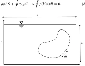
For an arbitrary control volume on the cross-section of a rectangular channel (Figure 1), assuming a steady uniform ow, the continuity and momentum equations can be written as follows:

I

(V:n)dl = 0; (1)

gAS + I

nxdl

I

u(V:n)dl = 0; (2) where is density and A is area of the control surface on y z plane, g is gravitational acceleration, S is channel slope, V is velocity component of ow on y z plane, n is unit normal vector pointing outside of the control volume, l is length along the boundary of surface, and nx is shear stress in the ow direction

x applying on the plane perpendicular to n. Flow velocity components u, , and w are in longitudinal, lateral, and vertical (i.e., x, y, and z) directions, respectively.

For a control volume surrounded by an isovel (i.e., constant u), the momentum equation (Eq. (2)) can be rewritten as follows:

gAS + I

nxdl u

I

(V:n)dl = 0: (3)

Figure 1. An arbitrary control volume in a channel cross-section.

Figure 2. Isovels and orthogonal curves for b=h = 2 (isovels are calculated following Chiu and Hsu, 2006 [26]).

Considering Eq. (1), the third term of Eq. (3), which represents the eect of secondary ows, vanishes and Eq. (3) reduces to:

gAS + I

nxdl = 0: (4)

Eq. (4) shows that the gravity component of a control volume limited to an isovel is balanced only by the shear stress acting on its surface due to velocity gradi-ents. On the other hand, if the momentum equation is applied to a control volume surrounded by two curves (polygon MNOM in Figure 2), which are orthogonal to isovels, one can write:

gAMNOMS +

I

MNOM

nxdl

I

MNOM

u(V:n)dl = 0; (5) where AMNOM is the area of the control volume

surrounded by the polygon MNOM, and both in-tegrals are calculated along the same polygon. The rst integral on the left-hand side of Eq. (5) can be calculated on subsections of the polygon MNOM as follows:

Z

MNOM

nxdl =

Z

MN

nxdl +

Z

NO

nxdl +

Z

OM

nxdl:

(6) nx can be assumed as follows:

nx= (t+ )_@n@u; (7)

where and t are kinematic and turbulent viscosity

of water, respectively. Since NO and OM are orthog-onal to isovels, @u=@n is zero along them; therefore, integrals R_NO and R_OM are zero, too. Considering the average shear stress on MN as MN, its length as

PMN, and Eq. (5), we can derive:

jMNj = _P1 MN

0

@gAMNOMS

I

MNOM

u(V:n) 1 A dl:

(8)

For a known 3D velocity eld, one can calculate the shear stress distribution on the channel boundary employing Eq. (8); however, usually, all 3 velocity components are not known. Note that viscosity does not show up in Eq. (8); however, its eects are considered through the velocity eld.

Based on the above discussion, shear resistance cannot be neglected neither on a control volume surrounded by isovels nor surrounded by orthogonal curves to isovels. Thus, it seems unlikely to nd a series of zero shear curves in the cross-section of an open channel. The channel centerline, however, is an exception at which both the shear resistance caused by secondary currents and velocity gradient are zero due to symmetry. If secondary currents are neglected, despite their indisputable eect, Eq. (8) becomes:

jMNj = gA_PMNOMS

MN : (9)

Eq. (9) describes Leighly's assumption, which is proved not be accurate. Guo and Julien [6] employed the same assumption to propose a rst approximation for mean shear stress on the channel bed and walls.

Regardless of the secondary currents, the dis-tribution of the main velocity, u, should be known to calculate the orthogonal curves to isovels and, consequently, the distribution of shear stress on the channel boundary. It is well known that, in an open channel, the maximum velocity may occur at a point below the water surface [19]. The location of the maximum velocity is important, because it is the point of concurrency of the isovel orthogonal trajectories.

Several researchers have proposed methods to calculate the velocity distribution in an open channel. The method of Maghrebi and Rahimpour [20], similar to that of Houjou and Ishii [21], predicts the location of the maximum velocity to be below the water surface for b=h < 2, where b is the channel width and h is the ow depth. This result is due to the fact that an open channel with b=h = 2 is half of a square conduit, in which the velocity prole is symmetrical in y and z directions [21]. De Cacqueray et al. [22], who examined the formulation of Guo and Julien [6] using a detailed computational uid dynamic simulation, reported that the maximum velocity occurs on the ow surface for a channel with b=h = 2 for their numerical experiments. However, it is widely reported that the dip phenomenon is observed for channels with b=h < 5 [23-25].

The velocity distribution proposed by Chiu and Hsu [26] is employed in the present paper to calculate the shear force distribution. Chiu and Hsu [26] presented an entropy-based approach to calculate the velocity distribution. This method relies on a pa-rameter which could be found according to various hydraulic parameters of the channel, such as the ratio of the average velocity to the maximum velocity and

the location of the maximum velocity. The location of the maximum velocity can be measured or calculated through the method from Yang et al. [27] as follows:

" h= 1

1

1 + 1:3e b=2h; (10)

in which " is the depth of the maximum velocity. The isovels and their orthogonal curves for a channel with b=h = 2 calculated by Chiu and Hsu [26] method based on Eq. (10) are shown in Figure 2. The slope of the isovel orthogonal trajectories at any point can be calculated from tan() = (@u=@z)=(@u=@y). Starting from a certain point on the boundary and following the slope, the orthogonal trajectories can be drawn. If the momentum exchange generated by the secondary currents on the isovel orthogonal curves is neglected, the gravity component of the mass surrounded by the closed polygon BOEB (Figure 2) remains unbalanced, which leads to the underestima-tion of the total shear force on the channel bound-ary.

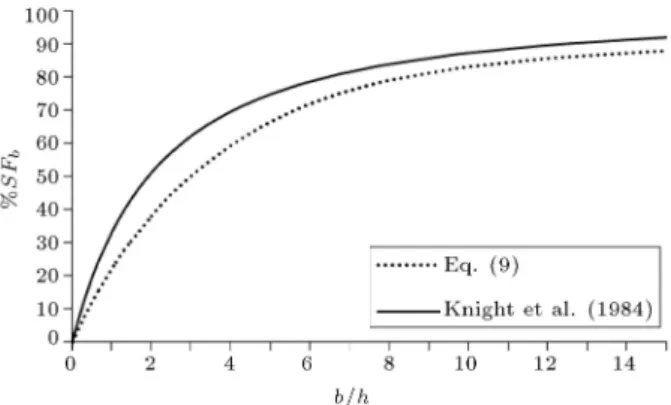
Figure 3 compares the estimation of Eq. (9) for %SFbwith the empirical equation presented by Knight

et al. [28]. As is illustrated in Figure 3, neglecting the secondary currents leads to underestimating the bed shear force and is not acceptable. The location of the maximum velocity moves toward the ow surface in wider channels; therefore, predictions of Eq. (9) become more accurate for larger b=h.

Figure 3. Comparison of %SFbpredicted by neglecting

secondary currents with the empirical equation presented by Knight et al. (1984) [28].

3. The present methodology

Eq. (8) can be employed to calculate the mean shear on the bed and sidewalls of an open channel if the eect of the secondary currents can be calculated. If the orthogonal trajectories to the isovels are drawn from the channel corners, they will intersect in the maximum velocity location (P2 curves in Figure 4).

The weight component of water in the area limited to P2 curves and channel bed, Ab min, must be less than

the shear force acting on the bed, since P2 curves are

orthogonal to isovels, with no velocity gradients and, consequently, no shear stress acting on them. However, there are secondary ows passing across these curves that cause momentum exchange. Secondary currents enter this area close to the channel centreline [19], where the main ow velocity is maximum. Due to the continuity, the ow entering this area close to the channel centerline leaves this area to locations where ow velocity is smaller. Therefore, the acting force due to the momentum transfer is in the ow direction. It will be shown later that the measured bed shear force is in excess of the weight component of the water in this area (Ab min).

Gessner and Jones [29] suggested that the sec-ondary ow cells in the corners of rectangular ducts are divided by the corner bisector. Experimental data presented by Tominaga et al. [30] show that secondary ows are strong in a region within a distance equal to 0:65h from the channel bottom corners. Zheng and Jin [31] and Jin et al. [32] assumed the same structure for corner secondary currents as Gessner [29] did in rectangular open channels, with the boundary of y=h = 0:65 and z=h = 0:65. It was assumed that the secondary ow cells have negligible eect on the ow mechanism out of this boundary [32]. The eective area of the secondary currents on the wall side can be, therefore, limited to the sidewall, bisector and a vertical line at y=h = 0:65 (region CJKBC, Figure 4). The weight component of water in this region must be less than the wall shear force, because it is assumed that secondary ows do not pass through the boundaries of this area; therefore, there is no momentum exchange due to secondary currents across these boundaries. However, there could be momentum exchange due to

the shear force in the ow. Since, in general, ow velocity decreases toward the sidewall, the shear force acting on the CJK is in the ow direction and its value is added to the weight component of CJKBC and does help balance it. This area, called Aw min, can be easily

calculated as follows: Aw min= 2

h + 0:35h

2 0:65h

= 0:65(1:35h2_{) 0:8h}2 _{for b=h>1:3:}

(11) In channels with b=h < 1:3, the corner bisectors intersect below z = 0:65h. This case will be discussed later.

According to these assumptions, CJK and P2 in

Figure 4 split the minimum share of sidewalls and bed from total shear force respectively. However, the weight component of the area between these two curves is assumed to be balanced partially by shear force acting on the sidewalls and partially with the shear force acting on the bed. The shared areas are divided into A1 and A2 by P1 curve (Figure 4). P1 is the

orthogonal curve to isovels drawn from upper corners of the channel cross-section. Let the share of the sidewalls from weight components of A1 and A2 be denoted by

1 and 2, respectively. One can, therefore, calculate

%SFw and %SFb as follows:

%SFW = _gAS2wh100%

= 100%_A

t (Aw min+ 1A1+ 2A2); (12)

%SFb=_gASbb 100%

=100%_A

t (Ab min+ (1 1)A1+ (1 2)A2₍₁₃₎);

where b and ware mean bed and wall shear stresses,

respectively, and Atis the channel cross-sectional area.

To determine 1and 2, A1and A2must be calculated

rst. To calculate these areas, equations for P1 and

P2 must be known. P1 can be approximated by a

parabola. P1 passes through (0; h) and (b=2; h ").

It is also perpendicular to the channel sidewall as an isovel; therefore, its derivative is zero in (0; h). The equation of P1 can therefore be written as follows:

z = "

(b=2)2y2+ h: (14)

Similarly, P2 passes through (0; 0) and (b=2; h ").

At the corner, P2 must be perpendicular to both the

channel bed and wall, which is not possible. To remove this conict, following Chiu and Chiou [13], the channel corner is assumed as a quarter circle; therefore, the slope of P2 in the corner is assumed equal to 1.

Contrary to P1, P2 cannot be approximated by

a parabola. A parabolic approximation signicantly deviates from P2 for larger b=h and may even exit

the water surface. To avoid this problem, P2 is

approximated by a parabola starting on the channel corner and a straight line following the parabola at a point to be determined, say (yi, zi). Considering these

boundary conditions, P2 can be expressed as follows:

z = a0_y2_{+ b}0_{y + c}0 _{y y}

i; (15a)

z = a00_{y + b}00 _{y > y}

i; (15b)

where: a0₌ zi yi

y2

i ; b

0_{= 1; c}0 _{= 0;}

a00₌ h " zi

b=2 yi ; b

00_{= h " a}00b

2:

The slopes of the parabola and the line are equal at their intersection point. This condition results in the following equation between yi and zi:

y2 i

zi+b₂+ (h ")

yi+ zib = 0: (16)

For a given zi, one can calculate yi from Eq. (16) and,

consequently, the unknown coecients a0_{, a}00_{, and b}00_.

zi is found by employing the least squares regression

between Eq. (15) and isovel orthogonal curves obtained based on Eq. (10). Plotting zi=(h ") against b=h

indicates that zi=(h ") is almost constant and can be

assumed equal to 0.93 for dierent values of b=h with about 2% averaged relative error. Figure 5 compares Eq. (15) with the Chiu and Hsu's [26] equations while assuming that zi=(h ") = 0:93.

Figure 5. Comparison of Eq. (15) for zi=(h ") = 0:93

with numerical data calculated through Chiu and Hsu (2006) method [26].

According to the equations found for P1 and P2,

A1 and A2 can be presented as follows:

A1= bh Aw min Ab min A2; (17)

Ab min= 2

a0_y3

i

3 + y2

i

2 +

zi+ h "

2

b 2 yi

; (18) A2= 2

b

6(" "0)

= ₃b(" "0_{) ; (19)}

where "0 _{is the vertical distance between the}

inter-section points of P1 and CJK from the water surface

(Figure 4). "0_{, shown in Figure 4, can be calculated}

from Eq. (16) as follows: "0₌ "

(b=2)2(0:65h)2: (20) The theory can be extended to b=h < 1:3 while considering necessary changes in the equations. For a channel with b=h < 1:3, the bottom corner bisectors intersect at the channel axis in a point like N, and two dierent patterns may occur (Figure 6). The maximum velocity may be below point N (Figure 6(a)), meaning that h " < b=2 < 0:65h. This pattern is similar to that of the channel cross-section with b=h > 1:3; however, Eqs. (11) and (19) must be substituted by Aw min = b(h b=4) and A2 0, respectively. The

maximum velocity may occur above point N, which means that b=2 < h " < 0:65h (Figure 6(b)). In this case, Aw min is limited to P2 and sidewall, and Ab min

is limited to the bisectors and channel bed and can, therefore, be easily calculated.

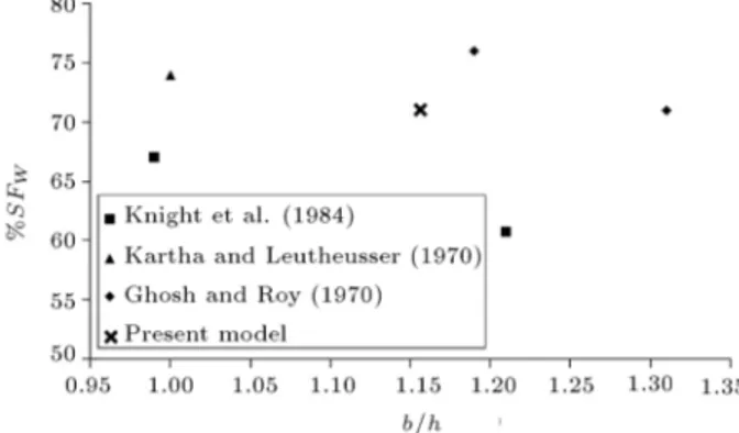
Employing Eq. (10) to calculate " shows that, in b=h = 1:16, point N conforms to point O. In this particular and interesting case, the bottom cor-ner bisectors and P2 conform and, therefore, can be

assumed as actual division lines across which there is no shear stress due to velocity gradient, or no momentum exchange due to secondary currents. In this case, 1 and 2 are eliminated from Eq. (12),

and %SFw is equal to %71. Figure 7 compares this

Figure 6. Possible cross-sectional division lines for b=h < 1:3.

Figure 7. Comparison of %SFw for b=h = 1:16 with

experimental results.

value with experimental results derived from dierent researches for b=h values close to 1.16. As seen from this gure, %SFw calculated from the present theory

is surrounded by the experimental results. A Gaussian weighted average from the shown experimental results in Figure 7 gives %SFw= 69% for b=h = 1:16 which is

very close to the predicted value of the present model. However, estimation of Knight et al.'s [25] empirical equation and Guo and Julien [15] is 63.2% and 62.9%, respectively.

4. Calibration

Figure 8 compares the result of Eq. (12) with experi-mental data presented by Knight et al. [28] from various researchers [33-39]. For 1= 2= 0, Eq. (12) gives the

minimum possible value of %SFw; for 1= 2 = 1, it

gives the maximum possible value of %SFw. It can be

seen in Figure 8 that the experimental data lie very well between the predicted minimum and maximum values for %SFw, which demonstrates the validity of

dividing the channel sections into Ab min and Aw min.

Contrary to the coecients used in previous related works, coecients 1and 2are physically meaningful

and limited to a range between 0 and 1. In addition, considering the maximum and minimum values of

Figure 8. Comparison of the present model for %SFw

%SFw illustrated in Figure 8, it can be seen that the

present model is not signicantly sensitive to the values of 1 and 2.

Employing the least squares method to estimate the share coecients results in 1 = 0:40 and 2 =

0:19 with the coecient of determination of R2_{= 0:98.}

According to these obtained values for 1and 2, %SFw

can be calculated from:

%SFw=100%_bh (Aw min+ 0:40A1+ 0:19A2); (21)

where Aw min, A1, and A2are calculated from Eqs. (11),

(17), and (19), respectively. In addition, %SFwvalues

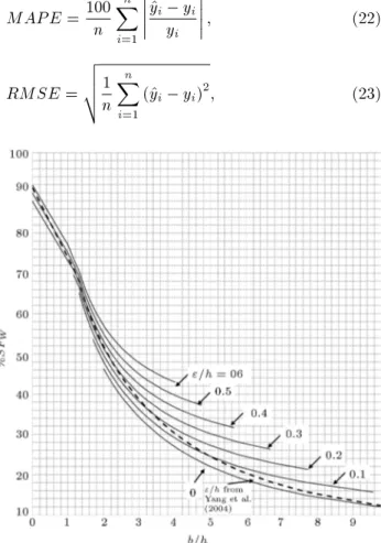
can be read from Figure 9 given the values of b=h and "=h.

5. Validation

The presented model is validated with several sets of unseen data, and the results are compared with predic-tions of Guo and Julien [6]. In order to measure how well each equation functions, Mean Absolute Percent-age Error (MAPE), Root-Mean-Square Error (RMSE), and Mean Signed Deviation (MSD) are utilized, which are dened as below:

MAP E =100_n Xn

i=1

^yi yi

yi

; (22)

RMSE = v u u t 1

n

n

X

i=1

(^yi yi)2; (23)

Figure 9. Values of %SFwfor dierent values of b=h and

"=h.

Figure 10. Comparison of the present model for %SFw

with unseen experimental data.

MSD = 1 n

n

X

i=1

^yi yi; (24)

where ^y is the predicted value of y, and n is the number of data points. MAPE and RMSE are measures of prediction accuracy, while MSD determines if a pre-diction method tends to underestimate or overestimate the values.

Figure 10 compares the present model (Eq. (21)) with experimental data of wall shear force from Seckin et al. [40] which are neither included in the calibration of the present model, nor in calibration of Guo and Julien [6] model. By excluding the experiment with b=h = 13:18 as an outlier, the MAPE for the present model is 4.7%, while it is 7.7% for Gou and Julien [6]. The RMSE of the present model is 0.63 and its value for Guo and Julien's model is 1.05. The MSD for both models is positive, which means that our model and Gou and Julien's overestimate %SFwwith mean values

of 0.46 and 0.93, respectively. Eq. (21) is, therefore, in very good agreement with the experimental data of Seckin et al. [40].

Results of comparison of the present model (Eq. (21)) and Gou and Julien (2005) with experi-mental measurements of Xie [41] and Chanson [42] for %SFware shown in Table 1. The MAPE for the present

model is 8.6%, while it is 9.3% for model of Gou and Julien [6].

Table 2 compares the result of Eq. (21) with experimental data of average bed shear velocity from experimental data of Coleman [43], Lyn [44,45], Muste and Patel [46], and predicted values by Gou and Julien [6]. The average bed shear velocity is calculated from ub =pb=. In this table, ub;mrepresents the

measured values, ub;21 is the results of Eq. (21), " is

calculated from Eq. (10), and ub;G&J is the prediction

of Gou and Julien [6]. It can be seen that the predicted values by the analytical models are slightly smaller than the measured values. This is due to the fact that the measured values are at a channel centreline; however, the predicated values are mean bed shear

Table 1. Comparison of the present model and Gou and Julien (G&J) [6] for %SFw with experimental data of

Xie [41] and Chanson [42].

b=h Measured G&J Eq. (21)

Xie [41] 3.2 36 36.40 36.62

Chanson [42]

2.9 38 39.26 39.62

3.24 37 36.05 36.25

5.32 19 23.35 22.98

5.95 18 20.99 20.50

MAPE 9.3 8.6

RMSE 2.47 2.26

MSD 1.61 1.59

velocities. The MAPE between results of Eq. (21) and experimental data is 3.23%, while it is 3.48% for model of Gou and Julien [6].

Coleman [43,47] reported the experiments con-ducted in a channel with S = 2 103_{, b = 35:6 mm,}

and Q = 0:64 m3_{/s, where S is the bottom slope and Q}

is the channel discharge. The experiments are carried out to investigate the eect of sediment suspension on a velocity prole. Coleman reported the location of maximum velocity in all experiments which can, therefore, be used directly in Eq. (21).

Table 3 compares the results calculated from the present method and model of Guo and Julien [6] with experimental data of Coleman [43]. In this table, ub;21is the result of Eq. (21) by directly substituting

" into the experiment. The total amount of sand suspended in the ow is given in this table in Kg as Ms. Moreover, the average volumetric suspended

sediment concentration (') of ow is calculated from available data in Coleman [43] and is provided in the table. It can be seen that the present model often

predicts the average shear velocities to be equal to or slightly smaller than ub;m; however, ub;G&J is

always larger than ub;m. The predicted mean values,

as mentioned before, should be slightly smaller than the measured local values since the measurements are made at the channel centreline. The measured shear velocities are almost constant and equal to 4.1 cm/s, though the aspect ratio of the channel is not constant. This is because velocity prole in each experiment also changes due to dierent sediments in suspension. The results, therefore, show that the bed shear velocity of an open channel is not only a function of the channel aspect ratio, but also a function of the location of the maximum velocity. The present model successfully captures this fact. It is, therefore, concluded that the present model can be extended to other ow conditions if the location of maximum velocity is known. The model can be eectively used for the sidewall correction procedure in ume studies, because, normally, in these studies, some experimental information on ow is available which can help estimate ". In cases where the pattern of the velocity distribution is dierent, e.g., in trapezoidal or vegetated channels, the idea of the current research is still applicable by modifying the boundaries of Aw min and Ab min. The equations for

P1 and P2 might also change based on the velocity

distribution.

It should be noted that the present method could be used as far as the location of maximum velocity, ", is known. " may be available in experiments or can be calculated based on other hydraulic parameters of an open channel ow using a graph presented by Chiu and Hsu [26]. While the equations proposed in the present research are derived for rectangular open channels, the proposed method of dividing the channel cross-section into subsections can be developed for channels with other cross-sectional shapes. Knight et

Table 2. Comparison of the present model for bed shear velocities (cm/s) with experimental data. S 103 _{b=h u}

b;m ub;21 ub;G&J

Coleman (1986) [43] Run 1 2 2.07 4.1 4.08 4.14 Lyn

(1986, 2000) [44; 45]

C1 2.06 4.08 3.1 3.05 3.05

C2 2.7 4.09 3.7 3.49 3.49

C3 2.96 4.64 3.6 3.51 3.5

C4 4.01 4.69 4.3 4.07 4.06

Muste and Patel (1997) [46]

CW01 0.739 7 2.92 2.79 2.78

CW02 0.768 7.1 2.92 2.83 2.82

CW03 0.813 7.16 2.98 2.9 2.89

MAPE 3.23 3.48

RMSE 0.13 0.14

Table 3. Comparison of the present model for bed shear velocities (cm/s) with experimental data from Coleman [43] for ow with suspended sediment.

Run Ms

(kg) '10

4 h

(cm) b=h

h " (cm)

ub;m

(cm/s)

ub;21

(cm/s)

ub;G&J

(cm/s)

1 0 0 17.2 2.070 13.2 4.1 4.14 4.14

2 0.91 2.12 17.1 2.082 12.0 4.1 4.09 4.14

3 1.82 3.87 17.2 2.070 11.9 4.1 4.09 4.14

4 2.73 5.87 17.1 2.082 12.8 4.1 4.12 4.14

5 3.64 8.03 17.1 2.082 12.2 4.1 4.10 4.14

6 4.54 9.76 17.0 2.094 11.9 4.1 4.08 4.13

7 5.45 12.22 17.1 2.082 12.0 4.1 4.09 4.14

8 6.36 14.37 17.3 2.058 13.0 4.1 4.14 4.15

9 7.27 16.29 17.2 2.070 13.6 4.1 4.16 4.14

10 8.18 18.56 17.1 2.082 13.4 4.1 4.15 4.14

11 9.09 20.34 16.9 2.107 12.2 4.1 4.10 4.13

12 10 21.69 17.3 2.058 13.4 4.1 4.15 4.15

13 10.91 23.92 17.1 2.082 12.2 4.1 4.10 4.14

14 11.82 25.64 17.1 2.082 12.2 4.1 4.10 4.14

15 12.73 21.51 17.1 2.082 11.9 4.1 4.09 4.14

16 13.64 28.39 17.1 2.082 11.2 4.1 4.06 4.14

17 14.54 23.15 17.1 2.082 13.1 4.1 4.14 4.14

18 15.45 28.56 17.2 2.070 13.1 4.1 4.14 4.14

19 16.36 30.16 17.0 2.094 13.1 4.1 4.13 4.13

20 17.27 31.24 17.0 2.094 12.6 4.1 4.11 4.13

21 0 0 16.9 2.107 12.8 4.1 4.12 4.13

22 0.91 1.80 17.0 2.094 12.2 4.1 4.10 4.13

23 1.82 3.45 17.0 2.094 11.9 4.1 4.08 4.13

24 2.73 5.27 16.9 2.107 12.2 4.1 4.10 4.13

25 3.64 7.08 16.7 2.132 10.4 4.0 4.01 4.12

26 4.54 8.84 17.1 2.082 13.0 4.1 4.13 4.14

27 5.45 10.37 16.8 2.119 12.2 4.1 4.09 4.12

28 6.36 12.00 17.0 2.094 12.2 4.1 4.10 4.13

29 7.27 13.65 16.8 2.119 13.0 4.0 4.13 4.12

30 8.18 15.00 16.8 2.119 13.7 4.1 4.16 4.12

31 9.09 15.93 17.2 2.070 11.9 4.1 4.09 4.14

32 0 0 17.3 2.058 13.1 4.1 4.14 4.15

33 0.91 0.42 17.4 2.046 12.8 4.1 4.13 4.15

34 1.82 0.71 17.2 2.070 13.1 4.1 4.14 4.14

35 2.73 1.16 17.2 2.070 12.2 4.1 4.10 4.14

36 3.64 1.89 17.1 2.082 12.2 4.1 4.10 4.14

37 4.54 2.30 16.7 2.132 11.9 4.1 4.08 4.12

MAPE 0.596 1.013

RMSE 0.035 0.046

al. [48] and Knight and Sterling [49] provided interest-ing information about the secondary current structures and velocity distribution in trapezoidal channels and circular partially full channels, respectively. Khozani et al. [5] also studied the shear distribution in circular and trapezoidal channels. Tang and Knight [50] and Yang et al. [51] studied the ow pattern in compound open channels with regular and vegetated ows, respectively. These works can be handy for researchers who might be interested in applying our method to other cross-sectional shapes or other ow regimes.

6. Conclusion

In the present paper, the channel cross-section was divided into parts using channel bisectors, at which shear force associated with secondary ows was zero and isovel orthogonal trajectories, at which shear force associated with velocity gradients was zero. The weight component of water in each of these subsections should be balanced either with bed or wall shear force. Based on these subsections, the minimum and maximum possible shear forces on walls and bed were calculated. The experimental data presented by various researchers lay well between the suggested maximum and minimum values. Considering the secondary ow structure, the share of the wall and bed from dierent subsections was calculated. An equation was nally derived for %SFw

and %SFb. Calculated wall and bed shear forces were

in good agreement with experimental data with a mean absolute percentage error of less than 5%.

The presented method can be used where the location of maximum velocity, ", is known. " is available in experiments, or can be calculated directly from empirical dip equations or indirectly from velocity prole laws in case of no velocity data. The depen-dence of our equations on " makes it applicable to a wide range of steady-uniform open channel ows. In addition, the proposed equations were applied to ows with suspended sediment, at which the location of the maximum velocity was known with good agreement. While our equations work only for rectangular chan-nels, the general concept is applicable to channels with dierent cross-sections.

Nomenclature

A Area of the control surface Ab min,

Aw min,

A1; A2

Subsections on the channel cross-section

Q Discharge

R2 _{Determination coecient}

S Channel slope

%SFb Percentage of the total shear force

acting on the bed

%SFw Percentage of the total shear force

acting on the walls

V Velocity component of ow on y z plane

b Channel width

" Depth of the maximum velocity h Water depth

g Gravitational acceleration

l Length along the boundary of surface n Unit normal vector pointing outside of

the control volume

1; 2 Parameters related to A1 and A2,

respectively

Density

' Volumetric suspended sediment concentration

b; w Mean bed and wall shear stress,

respectively

u; ; w Components of mean velocity in x, y, and z directions, respectively

ub;G&J Shear velocity predicted by Gou and

Julien (2005)

ub;m Experimentally measured shear

velocity

Kinematic viscosity t Turbulence viscosity

ub Mean shear velocity on bed

nx Shear stress in the ow direction x

applying on the plane perpendicular to n

x Longitudinal coordinate y Vertical coordinate z Spanwise coordinate References

1. Hamedi, A. and Ketabdar, M. \Energy loss estimation and ow simulation in the skimming ow regime of stepped spillways with inclined steps and end sill: A numerical model", Int. J. Sci. Eng. Appl., 5(7), pp. 399-407 (2016).

2. Bardestani, S., Givehchi, M., Younesi, E., Sajjadi, S., Shamshirband, S., and Petkovic, D. \Predicting turbulent ow friction coecient using ANFIS tech-nique", Signal, Image Video Process, 11(2), pp. 341-347 (2017).

3. Khozani, Z.S., Bonakdari, H., and Zaji, A.H. \Appli-cation of a soft computing technique in predicting the percentage of shear force carried by walls in a rectangu-lar channel with non-homogeneous roughness", Water Sci. Technol., 73(1), pp. 124-129 (2016).

4. Khozani, Z.S., Bonakdari, H., and Zaji, A.H. \Applica-tion of a genetic algorithm in predicting the percentage of shear force carried by walls in smooth rectangular channels", Measurement, 87, pp. 87-98 (2016). 5. Sheikh, Z. and Bonakdari, H. \Prediction of boundary

shear stress in circular and trapezoidal channels with entropy concept", Urban Water J., 13(6), pp. 629-636 (2016).

6. Guo, J. and Julien, P.Y. \Shear stress in smooth rectangular open-channel ows", J. Hydraul. Eng., 131(1), pp. 30-37 (2005).

7. Termini, D. \Momentum transport and bed shear stress distribution in a meandering bend: Experi-mental analysis in a laboratory ume", Adv. Water Resour., 81, pp. 128-141 (2015).

8. Yang, S.-Q. and Lim, S.-Y. \Mechanism of energy transportation and turbulent ow in a 3D channel", J. Hydraul. Eng., 123(8), pp. 684-692 (1997). 9. Heydari, H., Zarrati, A.R., and Tabarestani, M.K.

\Bed form characteristics in a live bed alluvial chan-nel", Sci. Iran. Trans. A, Civ. Eng., 21(6), pp. 1773 (2014).

10. Cheng, N.-S. and Chua, L.H. \Comparisons of sidewall correction of bed shear stress in open-channel ows", J. Hydraul. Eng., 131(7), pp. 605-609 (2005). 11. Guo, J. and Julien, P.Y. \Boundary shear stress in

smooth rectangular open-channels", In Advances in Hydraulics and Water Engineering, Proc. 13th IAHR-APD Congress, pp. 76-86 (2002).

12. Leighly, J.B., Toward a Theory of the Morphologic Signicance of Turbulence in the Flow of Water in Streams, University of California Press (1932). 13. Chiu, C.-L. and Chiou, J.-D. \Structure of 3-D ow in

rectangular open channels", J. Hydraul. Eng., 112(11), pp. 1050-1067 (1986).

14. Yang, S.-Q. \Interactions of boundary shear stress, secondary currents and velocity", Fluid Dyn. Res., 36(3), pp. 121-136 (2005).

15. Einstein, H.A. \Formulas for the transportation of bed load", Trans. ASCE Pap., 2140, pp. 561-597 (1942). 16. Keulegan, G.H., Laws of Turbulent Flow in Open

Channels, National Bureau of Standards US (1938). 17. Schlichting, H. \Experimental investigation of the

problem of surface roughness", Ingenieur-Archiv, 7(1), pp. 1-34 (1937).

18. Nezu, I. and Nakagawa, H. \Turbulence in open-channel ows", Vol. Monograph Series, Balkema, Rot-terdam: International Association for Hydraulic Re-search (1993).

19. Henderson, F.M., Open Channel Flow, Macmillan (1996).

20. Maghrebi, M.F. and Rahimpour, M. \A simple model for estimation of dimensionless isovel contours in open channels", Flow Meas. Instrum., 16(6), pp. 347-352 (2005).

21. Houjou, K. and Ishii, C. \Calculation of boundary shear stress INi open channel ow", J. Hydrosclence Hydraul. Eng., 8(2), pp. 21-23 (1990).

22. De Cacqueray, N., Hargreaves, D.M., and Morvan, H.P. \A computational study of shear stress in smooth rectangular channels", J. Hydraul. Res., 47(1), pp. 50-57 (2009).

23. Bonakdari, H., Larrarte, F., Lassabatere, L., and Joan-nis, C. \Turbulent velocity prole in fully-developed open channel ows", Environ. Fluid Mech., 8(1), pp. 1-17 (2008).

24. Nezu, I. and Rodi, W. \Open-channel ow measure-ments with a laser Doppler anemometer", J. Hydraul. Eng., 112(5), pp. 335-355 (1986).

25. Wang, X., Wang, Z.-Y., Yu, M., and Li, D. \Velocity prole of sediment suspensions and comparison of log-law and wake-log-law", J. Hydraul. Res., 39(2), pp. 211-217 (2001).

26. Chiu, C.-L. and Hsu, S.-M. \Probabilistic approach to modeling of velocity distributions in uid ows", J. Hydrol., 316(1), pp. 28-42 (2006).

27. Yang, S.-Q., Tan, S.-K., and Lim, S.-Y. \Velocity distribution and dip-phenomenon in smooth uniform open channel ows", J. Hydraul. Eng., 130(12), pp. 1179-1186 (2004).

28. Knight, D.W., Demetriou, J.D., and Hamed, M.E. \Boundary shear in smooth rectangular channels", J. Hydraul. Eng., 110(4), pp. 405-422 (1984).

29. Gessner, F.B. and Jones, J.B. \On some aspects of fully-developed turbulent ow in rectangular chan-nels", J. Fluid Mech., 23(04), pp. 689-713 (1965). 30. Tominaga, A., Nezu, I., Ezaki, K., and Nakagawa,

H. \Three-dimensional turbulent structure in straight open channel ows", J. Hydraul. Res., 27(1), pp. 149-173 (1989).

31. Zheng, Y. and Jin, Y.-C. \Boundary shear in rectan-gular ducts and channels", J. Hydraul. Eng., 124(1), pp. 86-89 (1998).

32. Jin, Y.-C., Zarrati, A.R. and Zheng, Y. \Boundary shear distribution in straight ducts and open chan-nels", J. Hydraul. Eng., 130(9), pp. 924-928 (2004). 33. Cru, R.W. \Cross-channel transfer of linear

momen-tum in smooth rectangular channels", No. 1592-B. USGPO (1965).

34. Ghosh, S.N. and Roy, N. \Boundary shear distribution in open channel ow", J. Hydraul. Div., 96(HY4), Proc. Paper 7241, pp. 967-994 (1970).

35. Kartha, V.C. and Leutheusser, H.J. \Distribution of tractive force in open channels", J. Hydraul. Div., 96(HY 7), Proc. Paper 7415, pp. 1469-1483 (1970). 36. Knight, D.W. and Macdonald, J.A. \Hydraulic

resis-tance of articial strip roughness", J. Hydraul. Div., 105(6), pp. 675-690 (1979).

37. Knight, D.W. and Macdonald, J.A. \Open channel ow with varying bed roughness", J. Hydraul. Div., 105(9), pp. 1167-1183 (1979).

38. Knight, D.W. \Boundary shear in smooth and rough channels", J. Hydraul. Div., 107(7), pp. 839-851 (1981).

39. Myers, W.R.C. \Momentum transfer in a compound channel", J. Hydraul. Res., 16(2), pp. 139-150 (1978). 40. Seckin, G., Seckin, N., and Yurtal, R. \Boundary shear stress analysis in smooth rectangular channels", Can. J. Civ. Eng., 33(3), pp. 336-342 (2006).

41. Xie, Q. \Turbulent ows in non-uniform open chan-nels: experimental measurements and numerical mod-elling", PhD Thesis, Department of Civil Engineering, The University of Queensland (1998).

42. Chanson, H. \Boundary shear stress measurements in undular ows: Application to standing wave bed forms", Water Resour. Res., 36(10), pp. 3063-3076 (2000).

43. Coleman, N.L. \Eects of suspended sediment on the open-channel velocity distribution", Water Resour. Res., 22(10), pp. 1377-1384 (1986).

44. Lyn, D.A. \Turbulence and turbulent transport in sediment-laden open-channel ows", Dissertation (Ph.D.), California Institute of Technology (1987). 45. Lyn, D.A. \Regression residuals and mean proles

in uniform open-channel ows", J. Hydraul. Eng., 126(1), pp. 24-32 (2000).

46. Muste, M. and Patel, V.C. \Velocity proles for parti-cles and liquid in open-channel ow with suspended sediment", J. Hydraul. Eng., 123(9), pp. 742-751 (1997).

47. Coleman, N.L. \Velocity proles with suspended sedi-ment", J. Hydraul. Res., 19(3), pp. 211-229 (1981). 48. Knight, D.W., Omran, M., and Tang, X. \Modeling

depth-averaged velocity and boundary shear in trape-zoidal channels with secondary ows", J. Hydraul. Eng., 133(1), pp. 39-47 (2007).

49. Knight, D.W. and Sterling, M. \Boundary shear in circular pipes running partially full", J. Hydraul. Eng., 126(4), pp. 263-275 (2000).

50. Tang, X. and Knight, D.W. \Lateral depth-averaged velocity distributions and bed shear in rectangular compound channels", J. Hydraul. Eng., 134(9), pp. 1337-1342 (2008).

51. Yang, K., Cao, S., and Knight, D.W. \Flow patterns in compound channels with vegetated oodplains", J. Hydraul. Eng., 133(2), pp. 148-159 (2007).

Biographies

Sasan Tavakkol is a PhD candidate in the University of Southern California (USC), Los Angeles, USA. His PhD research concerns the development of an interac-tive real-time software for simulation and visualization of coastal waves. This software, called Celeris, is then employed along with crowdsourced data in disaster to increase situational awareness. He received his second MSc in computer science from USC where his research project was concerned with prioritizing crowdsourced data. Sasan obtained his BSc and rst MSc from Amirkabir University of Technology (AUT) with the highest GPA. His research topics at AUT include Smoothed Particle Hydrodynamics (SPH) and open channel ows.

Amir Reza Zarrati is a Professor of Hydraulic En-gineering at the Department of Civil and Environmen-tal Engineering, Amirkabir University of Technology Tehran, Iran. He has more than 20 years of teaching and research experience. His main area of research is numerical and physical modelling of ow behaviour in hydraulic structures and rivers. He is also interested in scouring phenomenon and methods of its control. Dr. Zarrati has also a long history of collaboration with the industry and has been a senior consultant in a number of large dams in the country. He is a member of Iranian Hydraulic Association (IHA) and International Association of Hydraulic Research (IAHR).