Pantoja, et al. Concrete International (2018) 40:9 - pp. 35-41
An Introduction to Deep
Learning
This technology will be used to enhance and improve identification of structural damage
by Maria Pantoja, Anahid Behrouzi, and Drazen Fabris
D
eep learning (DL) is a subset of machine learning, the science of using computers to improve performance without problem explicit programming. Thanks to recent advances in computer architecture, data acquisition and storage systems, and software tools, DL has become thedominant focus for artificial intelligence (AI) research and
development. The goal of this article is primarily to describe
the DL process and briefly illustrate an example that will
enable professional structural engineers to automatically label images. More detail on the example is provided in the references. Much DL research has been concentrated on the development of computer instructions (algorithms) to classify data. Many
DL algorithms have been designed to find and report patterns
in data without any preprocessing of these data—this DL application is known as unsupervised learning. Other DL algorithms learn from data sets (training sets) by correlating
patterns in the data with classifications provided by human
experts (ground truth data)—this DL application is known as supervised learning. Supervised learning is like learning with a teacher who tells you what is the right answer and guides you; unsupervised learning is like learning without a teacher
and your task is to find the patterns in the data on your own. In this article, the focus is only on supervised learning.
After training, DL algorithms become tools that are used to
categorize new data sets. Many of these DL models (generally termed algorithms) can assess data faster and more accurately than expert practitioners. For example, radiologists can now use DL algorithms to conduct analyses of images used for cancer detection.1 The algorithms are adept at identifying
incipient tumors and alerting the radiologists to the need for
closer examination. In another example, DL algorithms are
also being developed to allow unmanned aerial vehicles
(UAVs) to assist in inspection of civil infrastructure by
autonomously directing themselves to a pertinent structure,
then sub-areas in the structure, and then specific, probable
anomalies.2 Images created by these UAVs can then be
analyzed by yet another DL algorithm to automatically identify and tag structural damage. The resulting collection of tagged images can then be used by structural engineers to determine appropriate actions.3,4 Similar technologies can also
be used to train machines capable of autonomously working in hazardous environments5 or to manage inventory in civil
infrastructure projects.6
The future of image recognition in civil infrastructure will be enhanced by advancements in theory and capability of computer vision systems. This will not be a substitute for the knowledge of expert structural engineers; rather, by
highlighting damages in images, such DL algorithms will facilitate more rapid and targeted analysis by experts. DL solutions are currently being researched and implemented to
solve civil engineering related problems. As these techniques
become implemented by civil engineers around the world, DL can contribute to the surveying and improvement of
infrastructure on a larger scale.
The Deep Learning Process
OverviewDL algorithms are built from artificial neural networks (termed ANN or NN). In general, an NN is comprised of
interconnected nodes (called neurons) that are arranged in layers. While neurons within a particular layer are
independent of each other, the neurons in a layer are linked to the neurons in preceding and following layers by functions with variable weights. The term “neuron” was assigned to
nodes in NN because the multiplicity of connections between
nodes can be likened to the synaptic connections between neurons in a brain. For supervised learning algorithms, the
weights in the NN algorithm are determined during a training
step, by an iterative process that minimizes errors between
classifications made by the algorithm and classifications
Learned weights are used to classify new
images (a) (b) neuron j bi wi0 x1 xi-1 xi xi+1 xN wi1
wij wjk
wi2
...
...
yj yk
yj-1 yj+1 pixel data input image
Sum all differences to obtain training loss input
layer hiddenlayer damage type & locationNN output:
yj
Initialize all weights for all neurons in
all layers
Classify images in Training Set using the NN
Compare results of NN output with classification provided by expert
Add all errors to find LOSS
NN output
If loss is small--DONE Output is the set of weights If loss is not
sufficiently small
Classified by expert Update neuron weights using optimization techniques (a) (b)
be used to make predictions from new data. This learning process generally improves with increasing amounts and
quality of preclassified data used for training. The model weights are updated as new data are acquired and classified.
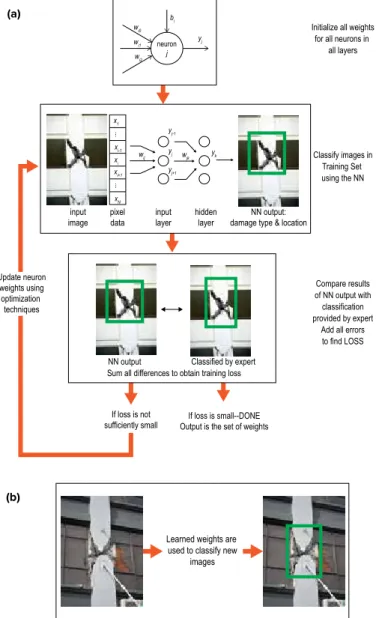
When developing an NN, two main steps are mandatory (Fig. 1). First, the NN is trained on a set of data that has been preclassified, generally by human experts. Training is an iterative process, in which the algorithm finds a set of weights
that minimizes an error measure. Without getting into the details, this training process combines linear algebra,
statistics, and differential calculus to minimize the error between the classifications assigned by the algorithm and classifications in ground truth data. Second, the trained NN, or model, is deployed to classify new data sets. The NN approach
(a) bi
neuron
j
w Initialize all weights
w y for all neurons in i0 j i1 all layers wi2 x1 xi-1 xi xi+1 xN
wij wjk
...
...
yj yk yj-1
yj+1
data image input pixel
Sum all differences to obtain training loss input
layer hidden layer damage type & location NN output:
NN output Classified by expert
Classify images in Training Set using the NN
Update neuron Compare results weights using
of NN output with optimization
techniques classification provided by expert
Add all errors to find LOSS
If loss is not If loss is small--DONE sufficiently small Output is the set of weights
Learned weights are used to classify new
images
(b)
Fig. 1. Basic workflow for a DL algorithm designed to identify damage in images of structures: (a) in the training step, the algorithm sets internal parameters (weights) based on images tagged by an expert as showing damage or no damage; and (b) in the deployment step, the trained model is used to identify damage in new images
can be used to classify text, images, or other information. In this article, however, we will focus on classification of
images, which is a machine vision application.
As statedpreviously, DLalgorithms mimic the connectivity
of biological neural systems. Although we do not exactly
know how the human brain works, we do know that a collection of connected neurons can perform very complex tasks, even though a single neuron can do very little. The same can be said about the connected neurons in a DL algorithm. The neurons in a DL algorithm can mimic a
biological neuron by “firing” when stimulated sufficiently by
inputs from other neurons. We term this activation and the mathematical operators that determine the state of a neuron are termed activation functions.
DL algorithms are trained by iteratively making
calculations forward and backward through the network. The
training step in developing an NN is an iterative process that effectively calibrates a model. This is illustrated in Fig. 1(a).
During a forward pass, the training set is classified, or
assigned a score, by the algorithm using the current network weights. During a backward pass, the weights are updated to
improve the classification relative to the ground truth on the
next iteration. The adjustments are made using loss and cost
functions to measure the error between the classifications made by the algorithm and the classifications provided in the
training set. Detailed descriptions of loss functions can be found in the literature (for example, refer to Reference 7).
Neurons and weights
For DL applications, a neuron k is a software function that takes an input and generates an output using an activation function (Fig. 2(a)). Each neuron k has a bias bk and a set of
weights, wjk, associated with its connection to preceding
neurons i. The bias provides a uniform offset to control the
sensitivity of the learning process. The weights provide indications of the level of interaction between nodes.
Together, they can be considered as analogous to the intercept value and the slope in the equation for a straight line.
Whenever there is a change in the input xi the output varies linearly. As a starting point, the weights are usually initialized to small arbitrary values. The weights within the NN will
change during the iterative learning process.
Neurons are grouped in layers (Fig. 2(b)) that are
connected with other layers of neurons. In fact, deep learning
gets its name from the high number of layers used in DL
algorithms. An NN is comprised of an input layer that reads
input values and an output layer that produces one or more
numbers that represent a certain classification. An NN also
comprises multiple hidden layers (layers between input and
output layers). In a fully connected NN, each neuron adds all
the outputs of the previous layer’s neurons together and applies an activation function, whose job is to pass to the next layer these additions only if it is above a threshold value (again, the activation function determines if the neuron will
1st layer
“Edges”
2nd layer
ject parts”
3rd layer
“Objects”
(a) (b)
Fig. 2: Details of neurons and layers in an NN: (a) neuron k, with yj input values and output yk. For each neuron k, wjk is the weight assigned to
the neuron for each yj; and (b) schematic of layers in an NN, showing the position of neuron k within the red box
is too small, the neuron will not translate input from the previous layers to the following layers. The activation function determines whether the output from a layer’s neuron will identify and propagate an input. Some of the activation functions used in DL algorithms are discussed in Reference 8.
Training
During training, the weights and biases are adjusted for each neuron, allowing interconnected hidden layers to learn patterns from an input set. The number of neurons per hidden layer and the number of layers is chosen by the data engineer. The complexity of the model is usually based on some
previously developed NN that was used to solve a similar
problem. The number of neurons in the input layer is the same as the size of the input data. For example, if the input
comprises 32 x 32-pixel greyscale images, the input layer will contain 322 = 1024 neurons. Note that each pixel will have
256 tonal levels for a black-and-white image, and that the number of neurons in the input layer will triple if the input comprises red, green, and blue color images.
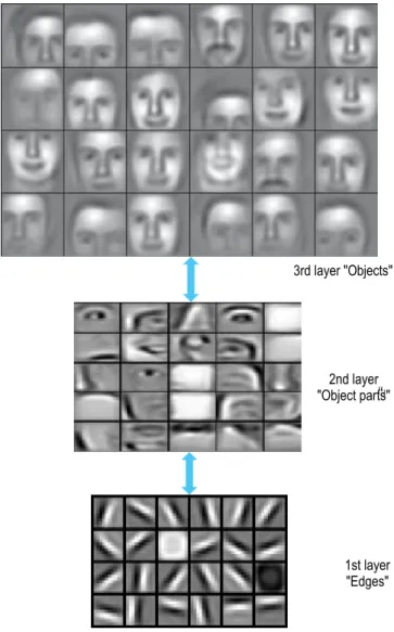
Successive hidden layers in NN algorithms have been
observed to be capable of progressively identifying
higher-level features. For example, the first hidden layer may identify
contrast lines within images (Fig. 3).9 The next hidden layer
may then respond to associations of these edges, with neuron connections that are sensitive to respectively identifying
noses, eyes, ears, and mouths, for example. A deeper layer
might then have neurons that are activated by the presence of a nose, two eyes, two ears, and a mouth (in other words, neurons in this layer would respond positively to a face). By connecting many layers, we can create systems that can learn to identify complex objects in an image (Fig. 3).
As previously stated, training the NN is an iterative process, with the goal of minimizing the classification errors
associated with the training set (ground truth). Massive numbers of weights and biases may be adjusted during the process, even if the algorithm provides only a binary (true or
false) classification. For example, if the input is a 32 x 32-pixel
3rd layer "Objects"
2nd layer "Object parts"
“Ob
1st layer "Edges"
greyscale image, the network will require 1024 neurons in each hidden layer to be fully connected (in a fully connected layer, all neurons in that layer are connected to all neurons in
the preceding and succeeding layers in the network). If the network configuration has 10 fully connected hidden layers,
over 855,000 weights must be adjusted during each training step, and each training step will include data for every image in the training set. Similarly, millions of weights must be learned for a DL algorithm with hundreds of layers and input images in the range of 1000 x 1000 pixels. Thus, DL algorithms can take hours to train, even using parallel processing accelerators such as graphics processing units (GPUs).
While a NN with many parameters can fit a training set
data very accurately, this does not necessarily mean that this
is a good solution for an implementation. Such a trained NN
may fail to generalize and thus will fail to correctly classify
new input images that differ from the images in the training set. This problem is called overfitting. Refer to Reference 8 for discussions of some of the methods used to avoid overfitting.
Classification errors associated with the training set are
determined using a loss function, which can be considered a surface in multi-dimensional space. This function is minimized using a very well-known optimization technique called gradient descent (GD),10 which finds changes in
weights that result in the steepest descent within the loss function to minimize the loss function.
This can be visualized using the function for the straight-line y = a + bx, where the slope b of the function is the rate of change (gradient), also given as the derivative of the function.
In the more general problem associated with DL, the gradient
Classification Competition
The Pacific Earthquake Engineering Research Center (PEER) has organized the first image-based structural damage identification competition, the PEER Hub ImageNet (PHI) Challenge. Contestants will receive
training and testing data sets that have been labeled for
classifications that include:
Scene level (pixel, object, or structural);
Damage condition (yes or no);
Spalling condition (yes or no);
Material type (steel or other);
Collapse state (none, partial, or full);
Component type (beam, column, wall, or other);
Damage level (none, minor, moderate, or heavy); and
Damage type (none, flexural, shear, or combined).Competitors will test the classification accuracy of their algorithms at three levels of difficulty. The
competition is scheduled to start on August 23 and close on November 25, 2018. The winner will be announced
on December 15, 2018.
Visit http://apps.peer.berkeley.edu/phichallenge/
for more information.
is the generalization of the slope for functions with a vector of input dimensions, and it must be found using partial
derivatives. While GD determines the direction in which the function has the steepest rate of change, the data engineer must determine how far the program should step. That is, the team developing the DL algorithm must heuristically set the
learning rate for the algorithm. If the steps are too large, the algorithm may overshoot the optimal solution. If the steps are too small, the algorithm will take too long to find a solution or
the algorithm might get stuck in a local minimum.
Because modern DL algorithms have millions of weights, calculation of the GD and the updates of the weights is so computationally intensive that DL algorithms were long
considered too slow and difficult to train. This changed when
Rumelhart, Hinton, and Williams described how to improve the convergence rate using backpropagation.11
Backpropagation is based on the chain rule and allows the calculation of the GD and the update of the input weights layer by layer. More details about back propagation are discussed in References 10 to 13.
The benefit of backpropagation is that the derivatives can
be calculated recursively and relatively quickly. Once the derivatives have been found, the weight on each neuron is adjusted proportionally, according to how fast that weight will
lower the loss function. The output of the classifier and the
gradients for each one of the neurons can be calculated to
minimize the loss function in one step. After this update is finished, the forward and backward passes are repeated until the loss value has satisfied a defined minimum. The output of the final training step will be the set of weights that minimize
the loss function.
Deployment or inference
The deployment step is much simpler than the training
step. Once the training step is finished, the result is a set of
weights that when multiplied by the input pixels will create
the automatic classification (Fig. 1), this step mainly consists in floating point multiplications and does not need
sophisticated hardware for intensive computation. Usually,
when a new NN is trained we use a computer that has one or
more GPUs, but the deployment can be executed by much simpler hardware, including smartphones, tablets, and smaller computing devices.
Convolutional Neural Networks
Convolutional neural networks (CNN) are a category of NN that have proven very effective in areas such as image recognition and classification. CNN derive their name from
the “convolution” operator, which reduces the number of weights required to classify the input. Compared to a
conventional NN, CNN networks reduce the computation
in the hidden layers by not requiring them all to be fully connected.
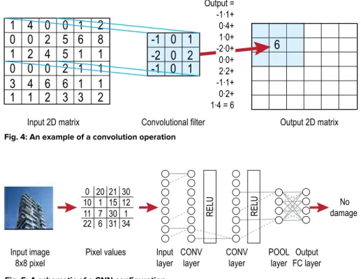
An image is a two-dimensional (2-D) matrix of pixel
filter is also a 2-D matrix, usually of
odd size (for example, 3 x 3 or 5 x 5).
A convolution operation is a
mathematical operation obtained by “sliding” (indexing) the convolutional
filter over every element in the input image matrix. At each position of the convolution filter the values in the filter
matrix are multiplied with the near neighbors in the image matrix and the products are summed (Fig. 4). Convolutions have been traditionally used in image processing to detect
edges and gradients. CNN algorithms
are designed to learn the values of these
convolution filters on theirownduring
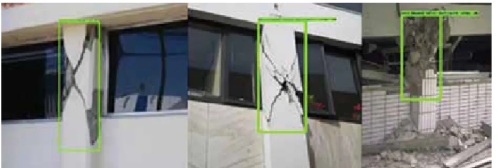
the training process. A commonCNN
configuration is illustrated in Fig. 5. In general, a CNN consists of a combination of the following layers:
INPUT layer, which comprises rawpixel values of an input image;
CONV layer, which will compute theInput 2D matrix Convolutional filter Output 2D matrix
1
1
1
-1
-1
0 0
0
0
0
0
0
0 0 0
1
1
3 3
3
2
2
2
2
-2
4
4
4
5
5
2
1 1
6 6
6
6
2
2
8
1 1
1 1
1 1
Output = -1˜1+ 0˜4+ 1˜0+ -2˜0+ 0˜0+ 2˜2+ -1˜1+ 0˜2+ 1˜4 = 6
Fig. 4: An example of a convolution operation
RELU RELU damage No
10 1 15 0
34
11 12
21
7 30
31 22 6 30 1
20
Input image Pixel values Input CONV CONV POOL Output
8x8 pixel layer layer layer layer FC layer
Fig. 6: Bounding box classification results: shear damage to short/captive column
output of neurons that are connected to local regions in the
inputs (RELU is short for rectified linear unit, an activation
function used in the computations);
POOL layer, which will perform a downsampling operation along the spatial dimensions (width, height); and
Fully Connected Output layer, which will compute the class scores for each category the algorithm is earning to recognize.The first work that widely popularized convolutional
networks in computer vision was the AlexNet.14 The AlexNet
was submitted to the ImageNet challenge in 2012,15 and it
significantlyoutperformed previous implementations. Infact,it
did so well, most of the DL algorithms for object classification are now CNN. CNN generalize well and can correctly classify different objects if enough preclassified input data can be
provided for training.
When creating a new NN to classify anewobject,thedata
engineer must decide the number of layers, the number of neurons per layer, the learning rate, and numerous other parameters. However, in practice, most practitioners reuse
previously trained CNN algorithms—they modify only a few
of the parameters for a new data set. This technique is called transfer learning.
One of the main goals of DL is to be able to automatically detect objects on image/video. This is based on the premise that if a human can see the
difference and manually tag/recognize
an object, then a DL algorithm should also be able to detect the same features and patterns needed to identify the
object. In our application, the object to
identify is a damage/structure pair on images taken after an earthquake. We have created a DL algorithm capable of recognizing earthquake-induced damage on concrete
buildings. For this process, we use the object detection
application programming interface for Tensorflow,15 a public
domain software package. Our implementation uses the
AlexNet configuration.14 The steps to develop the DL for
damage/structure defect detection are provided in Reference 15. The DL algorithm is capable of drawing a bounding box around short/captive column with shear damage, with an accuracy of 77%. Figure 6 presents a few examples of images the algorithm correctly tagged for this damage type.
There are a few challenges with training for specific
damage-structural member pairs that may explain the current
level of accuracy. First, finding 200 high-quality images from
reputable sources that accurately represent earthquake loading damage is a time-intensive process. Second, the research team is currently dependent on images tagged by only one expert.
There is a need to use multiple experts to provide verification of the ground truth set. Nevertheless, the current level of
accuracy is rather promising and we believe that with a larger set of training images labeled by at least two experts, the DL algorithm’s tagging performance would be comparable to a human expert. Output images would have additional metadata that includes the damage-structural member types and its locations in the images, which would enable large structural reconnaissance image repositories to become searchable using
specific terms.
Because this work is in the preliminary stages, we welcome
contributions from experts in the field to help build a
comprehensive database and implement and test the model.
Summary and Application
In this article, we presented an introduction to deep learning; specifically described is the use of a convolutional
neural network and the supervised learning process. This approach is currently being applied to train a model that will enable professional structural engineers to automatically
detect types of earthquake damage. Initial results are
promising. Output images would have additional metadata that includes the damage-structural member types and their locations in the images, which would enable large structural reconnaissance image repositories to become searchable using
specific terms.
learning have advanced to the stage that they can make
substantial improvement in many fields. DL solutions are
currently being researched and implemented to solve civil engineering related problems, including autonomous inspection and inventory of civil infrastructure projects.
References
1. Esteva, A.; Kuprel, B.; Novoa, R.A.; Ko, J.; Swetter, S.M.; Blau, H.M.; and Thrun, S., “Dermatologist-Level Classification of Skin Cancer
with Deep Neural Networks,” Nature, Feb. 2017, V. 542, No. 7639,
pp. 115-118.
2. Neurala, Inc., “Reducing Costs, Turnaround Time and Risk,” 2017,
10 pp.
3. Patterson, B.; Leone, G.; Pantoja, M.; and Behrouzi, A., “Deep Learning for Automated Image Classification of Seismic Damage to
Built Infrastructure,” Proceedings of the 11th National Conference in
Earthquake Engineering, 2018.
4. Behrouzi, A.; and Pantoja, M., “Photo Tagging Tool for Rapid and Detailed Post-Earthquake Structural Damage Identification,”
Proceedings of the 11th National Conference in Earthquake Engineering, 2018, poster presentation.
5. Lukka, T.J.; Tossavainen, T.; Kujala, J.V.; and Raiko, T.,
“ZenRobotics Recycler – Robotic Sorting Using Machine Learning,”
Sensor-Based Sorting, 2014, pp. 169-176.
6. Cohen, B.; Ye, S.; Karaman, G.; Khan, F.; Bartoli, I.; Pradhan, A.; Ellenberg, A.; Moon, F.; Gurian, P.; Antonios, K.; Minaeie, E.; Young, C.; Lowdemilk, D.; and Aktan, E., “Design and Implementation of an Integrated Operations and Preservation Performance Monitoring System
for Asset Management of Major Bridges,” 7th European Workshop on
Structural Health Monitoring, July 2014, pp. 1521-1528.
7. Janocha, K., and Czarnecki, W.M., “On Loss Functions for Deep Neural Networks in Classification,” arxiv:1702.05659, Feb. 2017, 10 pp., https://arxiv.org.
8. LeCun, Y.; Bengio, Y.; and Hinton, G., “Deep Learning,” Nature,
V. 521, May 2015, pp. 436-444.
9. Lee, H.; Grosse, R.; Ranganath, R.; and Ng, A., “Convolutional Deep Belief Networks for Scalable Unsupervised Learning of
Hierarchical Representations,” Proceedings of the 26th Annual International Conference on Machine Learning, 2009, pp. 609-616.
10. Rouder, S., “An Overview of Gradient Descent Optimization Algorithms,” arxiv:1609.04747, Sept. 2016, 12 pp., https://arxiv.org.
11. Rumelhart, D.; Hinton, G.; and Williams, R., “Learning
Representations by Back-Propagating Errors,” Nature, V. 323, Oct. 1986,
pp. 533-536.
12. Karpathy, A., “A Hackers Guide to Neural Networks,” http://
karpathy.github.io/neuralnets/.
13. LeCun, Y.; Bottou, L.; Bengio, Y.; and Hafner, P.,
“Gradient-Based Learning Applied to Document Recognition,” Proceedings of the
IEEE, V. 86, No. 11, Nov. 1998, pp. 2278-2324.
14. Krizhevsky, A.; Sutskever, I.; and Hinton, G., “ImageNet
Classification with Deep Convolutional Neural Networks,” Proceedings
of the 25th International Conferences on Neural Information Processing, Dec. 2012, pp. 1097-1105.
15. Abadi, M.; Barham, P.; Chen, J.; Chen, Z.; Davis, A.; Dean, J.; Devin, M.; Ghemawat, S.; Irving, G.; Isard, M.; Kudlur, M.; Levenberg, J.;
Monga, R.; Moore, S.; Murray, D.G.; Steiner, B.; Tucker, P.; Vasudevan, V.; Warden, P.; Wicke, M.; Yu, Y.; and Zheng, X., “TensorFlow: A System
for Large-Scale Machine Learning,” Proceedings of the 12th USENIX Conference on Operating Systems Design and Implementation, Nov. 2016,
pp. 265-283.
Selected for reader interest by the editors.
Maria Pantoja is an Assistant Professor in the Department of Computer Science and Software Engineering at California Polytechnic State University, San Luis Obispo, CA, and a Visiting Scholar with Sandia National Labs, Livermore, CA. Her area of research is high-performance computing and acceleration of computationally intensive algorithms, including computer vision and machine learning. She received her PhD in computer engineering from Santa Clara University, Santa Clara, CA. She is a member of the Association for Computing Machinery, IEEE, and the American Society for Engineering Education.
ACI member Anahid Behrouzi is an
Assistant Professor of Architectural Engineering at California Polytechnic State University. She is a member of ACI Committee 133, Disaster Reconnaissance, the ACI Student and Young Professional Activities Committee, and the ACI Foundation’s Scholarship Council. Her research interests include the earthquake performance of reinforced concrete structures and machine learning to further post-hazard structural reconnaissance. She received her MS and PhD in civil engineering at the University of Illinois at Urbana-Champaign, Urbana, IL.
Drazen Fabris is Chair and Associate Professor, Department of Mechanical Engineering, Santa Clara University. His research interests include the development of optical experimental
techniques in fluid dynamics and
thermal science, numerical modeling, testing thermal interface materials, and
developing non-contact reflectance based techniques for thin film and carbon nanostructure conductivity