Performance of the WRF model with different physical parameterizations in the precipitation simulation of the state of Puebla

(1)

Performance of the WRF model with different physical parameterizations in

the precipitation simulation of the state of Puebla

Indalecio MENDOZA URIBE1_{* and Diosey Ramón LUGO MORÍN}2

1 _{Subcoordinación de Hidrometeorología, Instituto Mexicano de Tecnología del Agua, Paseo Cuauhnáhuac 8532, Col.} Progreso, 62550 Jiutepec, Morelos, México.

2 _{Universidad Intercultural del Estado de Puebla, Calle Principal a Lipuntahuaca s/n, Col. Lipuntahuaca, 73475} Huehuetla, Puebla, México.

* Corresponding author; email: [email protected]

Received: November 15, 2018; accepted: January 24, 2020

RESUMEN

En México, las intensas lluvias generadas por ciclones tropicales, frentes fríos y sistemas convectivos de mesoescala pueden causar inundaciones y deslaves, los cuales provocan daños a los sectores sociales, de servicios, económicos y financieros, entre otros, y dejan a la población con menos recursos y en mayor vulnerabilidad. Dado este escenario, el tema de la prevención de desastres tiene relevancia en la agenda de protección civil, en la cual se reconoce que es indispensable establecer estrategias y programas de largo alcance enfocados a prevenir y reducir sus efectos y no sólo prestar atención a las emergencias y desastres. El objetivo de este trabajo es evaluar el desempeño del modelo WRF para simular la precipitación pluvial acumulada en 24 horas en el estado de Puebla, considerando 768 combinaciones diferentes de parámetros físicos, en comparación con los registros de lluvia de estaciones climatológicas para el periodo del 1 de junio al 20 de agosto de 2017. Además, como parte de la investigación, se definieron las configuraciones óptimas para obtener el mejor rendimiento del modelo a nivel local y estatal.

ABSTRACT

In Mexico, intense rains generated by tropical cyclones, cold fronts, and mesoscale convective systems can cause floods and landslides, causing damage to social, service, economic and financial sectors, among others, leaving the population with fewer resources and in greater vulnerability. Given this scenario, disaster prevention has relevance in the civil protection agenda, which recognizes that it is essential to establish long-range strategies and programs focused on preventing and reducing their effects, beyond only paying attention to emergencies and disasters. The objective of this work is to evaluate the performance of the WRF model for the simulation of accumulated pluvial precipitation in 24 hours in the state of Puebla, considering 768 different combinations of physical parameters, compared to rain records of weather stations for the period from June 1 to August 20, 2017. In addition, as part of the research, optimal configurations are defined to obtain the best performance of the model at local and state levels.

Keywords: WRF model, physical parameterizations, pluvial precipitation, state of Puebla.

1. Introduction

Mexico is located within the field of influence of tropical cyclones in its different scales (tropical depressions, tropical storms and hurricanes), that

(2)

the interior of the territory, causing loss of human life and considerable economic damage, which can sometimes have catastrophic tints (Aparicio, 1998; Douben, 2006). The increase in floods has occurred particularly in urban areas, negatively affecting the normal functioning of the social, service, economic and financial sectors, among others, leaving the population with fewer resources and in greater vul-nerability (Benjamín, 2008). In addition, Mexico is also frequently affected by other meteorological phenomena, such as cold fronts and mesoscale convective systems (Hernández-Uribe et al., 2017), independently of cyclonic activity.

The state of Puebla has historically presented the problem of flooding. The summary of damages caused by rains, floods, and tropical cyclones for the year 2008 amounted to 2070 people affected, 414 damaged homes and four deteriorated schools, adding economic damages for a total of 2.5 million pesos (SEGOB, 2009).

The Comisión Nacional del Agua (National Water Commission, CONAGUA) informed that rainfall recorded in the northern and northeastern mountains of the state of Puebla for August 10, 2017 as a result of Hurricane Franklin’s passage, broke various his-torical records. In the Zacapoaxtla weather station, 281 mm of rainfall were recorded, which exceeded the historical maximum of 204 mm recorded on August 9, 2012. Meanwhile, a precipitation of 225 mm was recorded at La Soledad station, a value that exceeds the historical maximum of 212 mm record-ed on August 8, 1979. Lastly, the Zaragoza station reported 198 mm of precipitation, higher than the historical maximum of 141.1 mm of August 5, 1975 (CONAGUA, 2017). The Atlas of water vulnerability to climate change in Mexico (Arreguín-Cortés et al., 2015), points out that the municipalities of Cuetzalan del Progreso and Zacapoaxtla, located in the north-west of the state, present a high risk given the current rainfall and tropical cyclone conditions.

In the face of this problem, Numerical Weather Prediction (NWP) constitutes a basic tool to un-derstand, explain and predict the behavior of the atmosphere. The Weather Research and Forecasting (WRF) model has a great acceptance and is used worldwide, both by the scientific community, aca-demics, predictors and decision makers. However, like other dynamic and statistical models, WRF is not

perfect, so it is necessary to evaluate its performance in each region. For the particular case of the state of Puebla, the performance of the WRF model for high spatial resolution forecasts of precipitation (which allows the quantitative determination of the degree of confidence and defines the set of optimal physical conditions) has not been evaluated.

The two main objectives of this research were to quantitatively evaluate the performance of the WRF model to simulate precipitation in the state of Pueb-la, considering different combinations of physical parameters, and compare the results with the rain records obtained from the weather stations during the summer of 2017; and to determine the optimal configurations of the WRF model for obtaining its best performance in the state of Puebla.

2. Dataset and methods

In the particular sense of the experimental approach, one or more independent variables are intentionally manipulated (alleged causes background) to analyze the consequences of this procedure on one or more dependent variables (supposed consequential effects) within a control situation for the researcher (Camp-bell and Stanley, 2012; Creswell, 2013; White and McBurney, 2013; Babbie, 2014; Hernández-Sampieri et al., 2014).

(3)

The spectrum of combinations of possible physi-cal parameters in the WRF model is very wide, more than 16 million in the ARW core. For this study, a total of 768 experimental groups were defined, each corresponding to the different levels of variation of the selected physical parameters.

To measure the effect of different experiments, statistical metrics were applied between the simulated precipitation and the accumulated rainfall records in 24 h in weather stations installed in the state of Puebla, where summers are rainier than other seasons of the year. For this reason, summer (from June 1 to August 20, 2017) was chosen as the study period. Further, during this time, the state of Puebla received the onslaught of Hurricane Franklin, which caused torrential rains that exceeded the historical highs in the state.

2.1. Study zone

The state of Puebla is located in the central part of Mexico. It borders to the north with the states of Hi-dalgo and Veracruz; to the east also with Veracruz and Oaxaca; to the south with the latter and Guerrero, and to the west with this state, Morelos, Mexico, Tlax-cala and Hidalgo (Tamayo, 1996). It has an area of 34 290 km2_{, which represents 17% of the total} nation-al space. It is characterized by a wide topographicnation-al heterogeneity because it houses four major biogeo-graphical provinces: The Sierra Madre Oriental, the coastal plain of the North Gulf, the Neovolcanic Axis, and the Sierra Madre del Sur. This geomorphological diversity causes marked changes in altitude, which give rise to a wide variety of climates, dominating the temperate climates that cover most of the terri-tory, followed by warm and semi-arid climates. The climatic heterogeneity is due, in part, to the fact that as altitude increases, temperature decreases and 65% of the territory of Puebla is composed of mountainous topography and hills.

2.2. Description of the WRF model

The performance of numerical models of weather pre-diction has increased in the last 40 years due mainly to four factors (Kalnay, 2003): (1) The increase in computing power of supercomputers, allowing a finer numerical resolution and fewer approximations in op-erational atmospheric models; (2) the improvement of the representation of small-scale physical processes

within the models (clouds, precipitation, turbulent heat transfer, humidity, momentum and radiation); (3) the use of more accurate data assimilation meth-ods, which results in an improvement of the initial conditions for the model, and (4) the increase in data availability, especially satellite and aircraft data on the oceans and the southern hemisphere.

The main features of the WRF model revolve around its non-hydrostatic dynamics and its ability to process spatial resolutions of a few kilometers (Moya-Álvarez and Ortega-León, 2015). About its structure, the WRF model has two dynamic cores (Advanced Research WRF [ARW] and Nonhydro-static Mesoscale Mode [NMM]), a data assimilation system, and a software architecture that allows the application of parallel computing to perform simu-lations (Skamarock et al., 2008). In this study, the dynamic core WRF-ARW version 3.9.1.1 was used. The WRF modeling system requires external data sources and consists of three main modules: (1) the WRF preprocessing system (WPS); (2) the ARW solver, and (3) third-party postprocessing and visu-alization tools.

2.3. Dataset

The forecast accuracy of the models lies primarily in a good description of the initial state of the atmosphere. This initial state, analysis or first approximation is created by an optimal combination between observed data and a short-term forecast derived from a previous analysis through a process known as data assimi-lation. According to Zepka (2011), for satisfactory results regarding the predictability of a storm or any adverse weather phenomenon characterized by very small spatial and time dimensions, high-quality input data with high temporal and spatial resolutions are necessary, as well as a high-resolution model.

The WRF model requires knowledge of the initial and boundary conditions for the simulation period at constant time intervals, information which is usu-ally incorporated from global data. For this study, we chose to use the data from the Global Forecast System (GFS) model, which is a reference for op-erational forecasting and research studies. GFS data was downloaded from ftp://ftp.ncep.noaa.gov/pub/ data/nccf/com/gfs/prod.

(4)

Surface Water and River Engineering Management of CONAGUA, through the site http://148.204.8.145. The HIS is a system sponsored by the World Mete-orological Organization (WMO) through the Water Management Modernization Program.

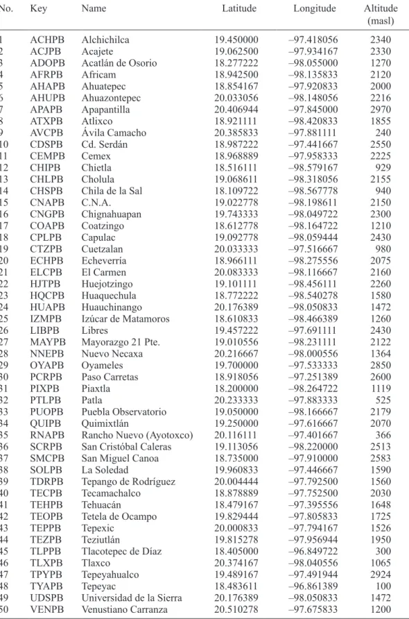
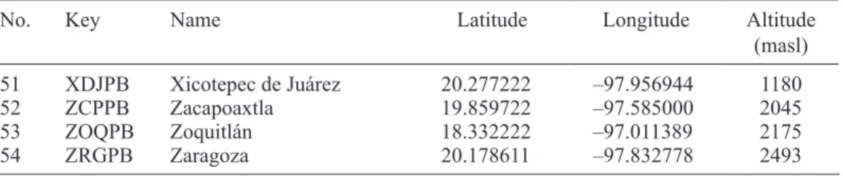
Fifty-four weather stations with at least 80% data in the study period were selected as sampling units. Table I lists the 54 selected weather stations with their corresponding keys, and Figure 1 their geographical location within the state of Puebla.

2.4. Experiment design

Two domains were defined for the execution of the WRF model, the mother domain with a spatial reso-lution of 16 km and a nested domain with a resoreso-lution of 8 km. Only simulated precipitation in the nested domain was used to evaluate the performance of the WRF model in the state of Puebla. Table II shows the fixed parameters selected for experimentation with the WRF model.

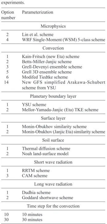
As mentioned above, 768 experiments with the WRF model were executed, each one corresponding to one of the possible combinations of the different physi-cal settings selected. Each parameterization was varied in two options, except for the convection parameteriza-tion, from which six different ones were selected since precipitation is directly associated with the formation of clouds. However, all the different physical param-eterizations affect the simulation of precipitation. The combination was selected on a discretionary basis of the compatibility at the run time between different combinations. Table III lists the physical parameters considered in the 768 experiments.

The results of the experiments were sorted by date and weather station, generating a text file consisting of 81 lines which corresponds to the analysis days of the period from June 1 to August 20, 2017. Each line contains 770 columns, the first one containing the date; the second column contains the observed pre-cipitation value, and columns 3 through 770 contain the precipitation value simulated by the WRF model in each of the 768 experiments.

2.5. Metrics to measure the performance of the WRF model

In systems modeling, an essential stage that presents both conceptual and practical difficulties is the validation of the models. An important part of this process is

empirical validation, which according to Reynolds (1984) and Mitchell (1997) is done to compare the predictions of the model with observations from the real world. According to Aguilar (1997) and Raus-cher et al. (2000), these comparisons should ideally be carried out using appropriate statistical methods, with an acceptable level of confidence, so that the inferences are correct (Barrales et al., 2004).

There are different methods to quantitatively vali-date numerical forecast models, highlighting the use of simple statistics of bias, root mean square error (RMSE) and Pearson correlation. These parameters were selected because they are not exclusive and can be used together. Among the works that propose and use these statistical parameters for the evaluation of forecast models are Willmott (1982), Pielke (1984), Willmott et al. (1985), Carbonell et al. (2003) and Das et al. (2015).

The selected statistics were applied to each obser-vation site for both the set of observed data (O) and model predictions (P). To the extent that the statistical indicators are favorable and show that the simulated data are approximate to observed data, and that the behavior over time of simulated variables is similar to that observed, it can be concluded that the simulation provides representative data and that the WRF model can simulate the precipitation in the state of Puebla (Gavidia, 2012).

RMSE is a measure of quantitative performance commonly used to evaluate forecasting methods. In this context, RMSE consists in the square root of the sum of the quadratic errors, which captures positive er-rors as negative; therefore, it expresses both systematic and random errors. RMSE amplifies and penalizes with greater force those errors of greater magnitude (Eq. 1).

RMSE = 1

∑

(Pi – Oi)2

√ n

n

i=1

(1)

where Pi is the prediction of the model in position i, Oi is the value observed in position i and n is the

sample size.

(5)

Table I. List of the 54 weather stations selected in the state of Puebla.

No. Key Name Latitude Longitude Altitude

(masl)

1 ACHPB Alchichilca 19.450000 –97.418056 2340

2 ACJPB Acajete 19.062500 –97.934167 2330

3 ADOPB Acatlán de Osorio 18.277222 –98.055000 1270

4 AFRPB Africam 18.942500 –98.135833 2120

5 AHAPB Ahuatepec 18.854167 –97.920833 2000

6 AHUPB Ahuazontepec 20.033056 –98.148056 2216

7 APAPB Apapantilla 20.406944 –97.845000 2970

8 ATXPB Atlixco 18.921111 –98.420833 1855

9 AVCPB Ávila Camacho 20.385833 –97.881111 240

10 CDSPB Cd. Serdán 18.987222 –97.441667 2550

11 CEMPB Cemex 18.968889 –97.958333 2225

12 CHIPB Chietla 18.516111 –98.579167 929

13 CHLPB Cholula 19.068611 –98.318056 2155

14 CHSPB Chila de la Sal 18.109722 –98.567778 940

15 CNAPB C.N.A. 19.022778 –98.198611 2150

16 CNGPB Chignahuapan 19.743333 –98.049722 2300

17 COAPB Coatzingo 18.612778 –98.164722 1210

18 CPLPB Capulac 19.092778 –98.059444 2430

19 CTZPB Cuetzalan 20.033333 –97.516667 980

20 ECHPB Echeverría 18.966111 –98.275556 2075

21 ELCPB El Carmen 20.083333 –98.116667 2160

22 HJTPB Huejotzingo 19.101111 –98.456111 2260

23 HQCPB Huaquechula 18.772222 –98.540278 1580

24 HUAPB Huauchinango 20.176389 –98.050833 1472

25 IZMPB Izúcar de Matamoros 18.610833 –98.466389 1260

26 LIBPB Libres 19.457222 –97.691111 2430

27 MAYPB Mayorazgo 21 Pte. 19.010556 –98.231111 2122

28 NNEPB Nuevo Necaxa 20.216667 –98.000556 1364

29 OYAPB Oyameles 19.700000 –97.533333 2850

30 PCRPB Paso Carretas 18.918056 –97.251389 2600

31 PIXPB Piaxtla 18.200000 –98.264722 1119

32 PTLPB Patla 20.233333 –97.883333 525

33 PUOPB Puebla Observatorio 19.050000 –98.166667 2179

34 QUIPB Quimixtlán 19.250000 –97.616667 2070

35 RNAPB Rancho Nuevo (Ayotoxco) 20.116111 –97.401667 366 36 SCRPB San Cristóbal Caleras 19.113056 –98.220000 2513

37 SMCPB San Miguel Canoa 18.735000 –97.910000 2583

38 SOLPB La Soledad 19.960833 –97.446667 1590

39 TDRPB Tepango de Rodríguez 20.004444 –97.792500 1560

40 TECPB Tecamachalco 18.878889 –97.752500 2030

41 TEHPB Tehuacán 18.479167 –97.395556 1648

42 TEOPB Tetela de Ocampo 19.829444 –97.805833 1725

43 TEPPB Tepexic 20.000833 –97.794167 1526

44 TEZPB Teziutlán 19.815278 –97.956944 1950

45 TLPPB Tlacotepec de Díaz 18.405000 –96.849722 300

46 TLXPB Tlaxco 20.374167 –98.040556 1065

47 TPYPB Tepeyahualco 19.489167 –97.491944 2924

48 TYAPB Tepeyac 18.483611 –96.861389 100

(6)

systematic error. Not having a bias or having a min-imal one is a desirable property which indicates that the forecast is close to reality (Eq. 2).

BIAS = 1n

∑

(Pi – Oi)2 = P – O n

i=1 (2)

Table I. List of the 54 weather stations selected in the state of Puebla.

No. Key Name Latitude Longitude Altitude

(masl) 51 XDJPB Xicotepec de Juárez 20.277222 –97.956944 1180

52 ZCPPB Zacapoaxtla 19.859722 –97.585000 2045

53 ZOQPB Zoquitlán 18.332222 –97.011389 2175

54 ZRGPB Zaragoza 20.178611 –97.832778 2493

México Puebla

D1

D2

Fig. 1. Geographical location of the selected weather stations in the state of Puebla (right). The station number corresponds to the list of stations in Table I. Experimentation domains with the WRF model (D1 [mother domain, red] and D2 [nested domain, orange]) are marked on the map of Mexico (left).

Table II. Fixed parameters selected for experimentation with the WRF model.

Parameter Description Mother domain Nested domain

dx Grid length in x direction (m) 16 000 8000

dy Grid length in y direction (m) 16 000 8000

map_proj Map projection Mercator Mercator

time_step Time step for integration in integer seconds 96 96 history_interval History output file interval (min) 180 60 ref_lat Central latitude of the mother domain 19.3453 19.3453

ref_lon Central length of mother domain –97.9065 –97.9065

e_we End index in x direction (west-east) 47 59

e_sn End index in y direction (south-north) 51 67

(7)

where Pi is the prediction of the model in position i, Oi is the value observed in position i, and n is the

sample size.

Pearson correlation, denoted by the letter r, is a normalized measure of the linear relationship between two continuous quantitative variables, that is, it measures the dependence of one variable with

respect to another independent variable. The Pearson correlation coefficient allows establishing similarities or dissimilarities between variables, to make evident the joint variability and therefore typify what hap-pens with the data (Mondragón-Barrera, 2014 ). The coefficient can score values ranging from –1.0 to 1.0. Values close to 1.0 indicate that there is a strong association between the variables, that is, when one increases the other as well. On the other hand, values close to –1.0 indicate that there is a strong negative association between the variables, implying that when one variable increases, the other decreases. When the value is 0.0, it indicates that there is no correlation, or the correlation is null (Anderson et al., 2008). In the correlation, the dependent variable is not distinguished from the independent one, so the correlation of O with respect to P is the same as the correlation of P with respect to O (Eq. 3).

r = ∑ (Oi – O)(Pi – P)

[∑(Oi– O)2] [∑(Pi– P)2]

√ √ (3)

where Oi is the value observed in position i, Pi is

the prediction of the model in position i, P̅ is the mean observed value, and P̅ is the mean model prediction.

The efficiency multiparameter index (EMI) was used to identify exposed cases with better perfor-mance at the state level, which involves four steps: 1. Calculation of the statistical metrics of bias,

RMSE and r in the 768 experimental groups of the 54 observation sites.

2. Assignment of weights to each experiment ac-cording to the level of efficiency in each of the three statistical metrics by location.

3. Application of the EMI (Eq. 4). EMI values range from 0 to 1, and are interpreted as deficient (0.0 < 0.2), regular (0.2 < 0.4), good (0.4 < 0.6), very good (0.6 < 8.0) and excellent (0.8 ≤ 1.0). 4. Selection of the experiment with the highest EMI

as a reference at the state level.

EMIe = _{ne * nl * nm}∑ Eelm (4)

where EMIe is the efficiency multiparameter index for experiment e, ne the number of experiments, nl

the number of locations, nm the number of metrics, and Eeml the weight of the experiment e for the metric

m and the location l. Table III. Physical parameters considered in the 768

experiments. Option

number Parameterization Microphysics 2 Lin et al. scheme

4 WRF Single-Moment (WSM) 5-class scheme Convection

1 Kain-Fritsch (new Eta) scheme 2 Betts-Miller-Janjic scheme 3 Grell-Devenyi ensemble scheme 5 Grell 3D ensemble scheme 6 Modifed Tiedtke scheme

14 New GFS simplified Arakawa-Schubert scheme from YSU

Planetary boundary layer 1 YSU scheme

2 Mellor-Yamada-Janjic (Eta) TKE scheme Surface layer

1 Monin-Obukhov similarity scheme

2 Monin-Obukhov (Janjic Eta) similarity scheme Soil surface

1 Thermal diffusion scheme 2 Noah land-surface model

Short wave radiation 1 RRTM scheme

3 CAM scheme

Long wave radiation 1 Dudhia scheme

2 Goddard shortwave scheme Time step for the convection 10 10 minutes

(8)

3. Results

3.1. Precipitation variability during the study

Given that the year 2017 presented a neutral ENSO condition, rainfall in the state of Puebla during the study period was normal with the exception of August 10, 2017 when in the northern and eastern regions of the state, precipitation from very strong to intense occurred with values exceeding 75 mm accumulated in 24 h. This extraordinary precipitation was caused by hurricane Franklin (category 1), which hit land on August 10 at 00:00 LT in the state of Veracruz and subsequently weakened at 4:00 LT to a tropical storm in the northern highlands of Puebla.

3.2. Analysis and interpretation of results

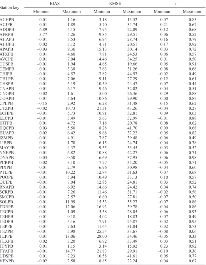
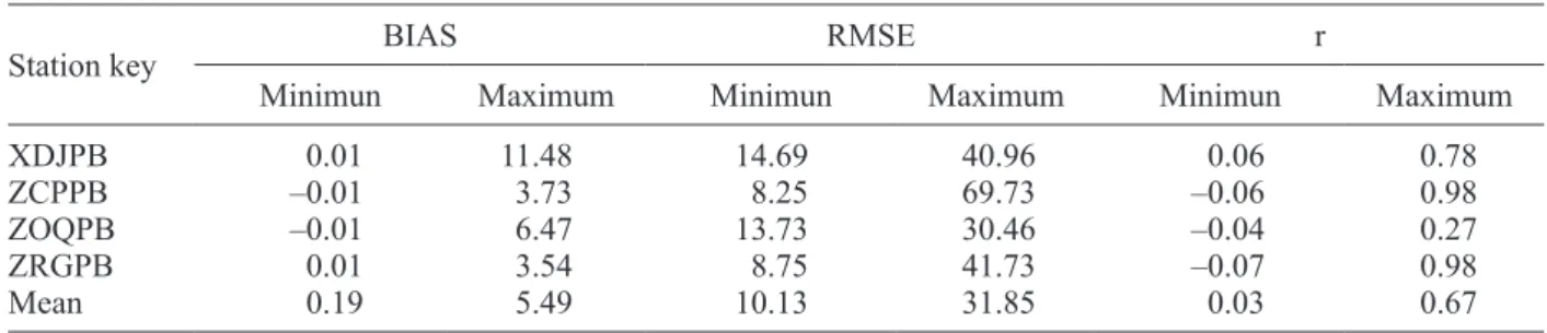
A first analysis was performed with the results of the statistical evaluation parameters in the 54 locations. Table IV shows the minimum and maximum values in the 768 experiments by weather station and sta-tistical metrics.

Overall, the 768 experiments tend to under-estimate precipitation with negative biases in 33 observation sites, positive biases with a tendency to overestimate precipitation in only six sites, and a mixed trend in 15 locations. Extreme biases in the 54 locations were presented in the interval [–41.96, 18.06].

On the other hand, the different experiments with the WRF model gave RMSEs in the interval [3.14, 69.73]. The lowest RMSE was obtained at ACHPB, AHUPB, CNGPB, CDSPB, TEHPB and TPYPB stations with intervals [3.18, 13.52], [4.71, 20.51], [5.0, 26.36], [4.65, 19.66], [4.02, 18.83], and [3.14, 15.92], respectively. At the opposite end, the WRF model presented the highest RMSE at the HJTPB and TLPPB stations with intervals [15.53, 55.27] and [8.25, 69.73], respectively.

Regarding the Pearson correlation parameter, the results are very varied in the same location. In the 768 experiments both negative and positive correlations were observed, the latter predominating. Under this metric, the WRF model achieved extremely high positive correlations with values greater than 0.9 at the AHUPB, CDSPB, OYAPB, TECPB, TEOPB, TPYPB, ZCPPB, and ZRGPB observation sites. Meanwhile, through the different 768 configu-rations, the lowest correlations were obtained at stations CTZPB, TEZPB and ZOQPB stations with

intervals of [–0.04, 0.27], [–0.08, 0.06] and [–0.04, 0.27], respectively.

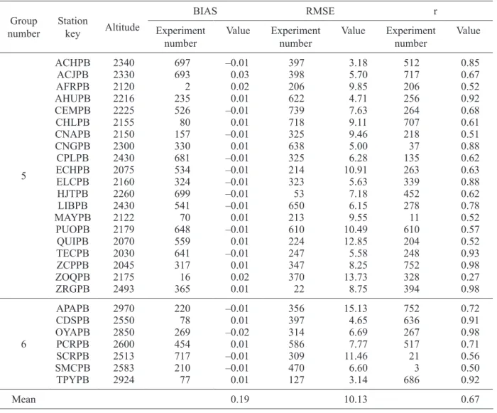
A second analysis of results was performed by grouping the observation sites into six groups with ranges of 500 masl, as shown in Table V. It was ob-served that at altitudes above 2000 masl, correspond-ing to groups five and six (which together concentrate 50% of the weather stations), the WRF model has bet-ter performance, especially in the central and northern region of the state of Puebla, with the exception of the ZOQPB station, where moderate performance was observed. The region in which the WRF model generally presented the lowest performance was the southwest of the state. The contrast between the 768 experimental groups in the same observation site is evident, starting with performances from low to very high. These results emphasize the importance of conducting experiments to determine the appro-priate configuration according to the study area. The exception is the CNGPB station, located to the north of the state of Puebla at an altitude of 2300 masl, where the WRF model in all experiments presented medium to very high performance, with bias in the interval [–11.85, 1.61], an RMSE maximum of 26.36 and r greater than 0.29; however, a bad configuration of the WRF model physical parameters in this station would not present, in statistical terms, serious errors in the simulation of precipitation.

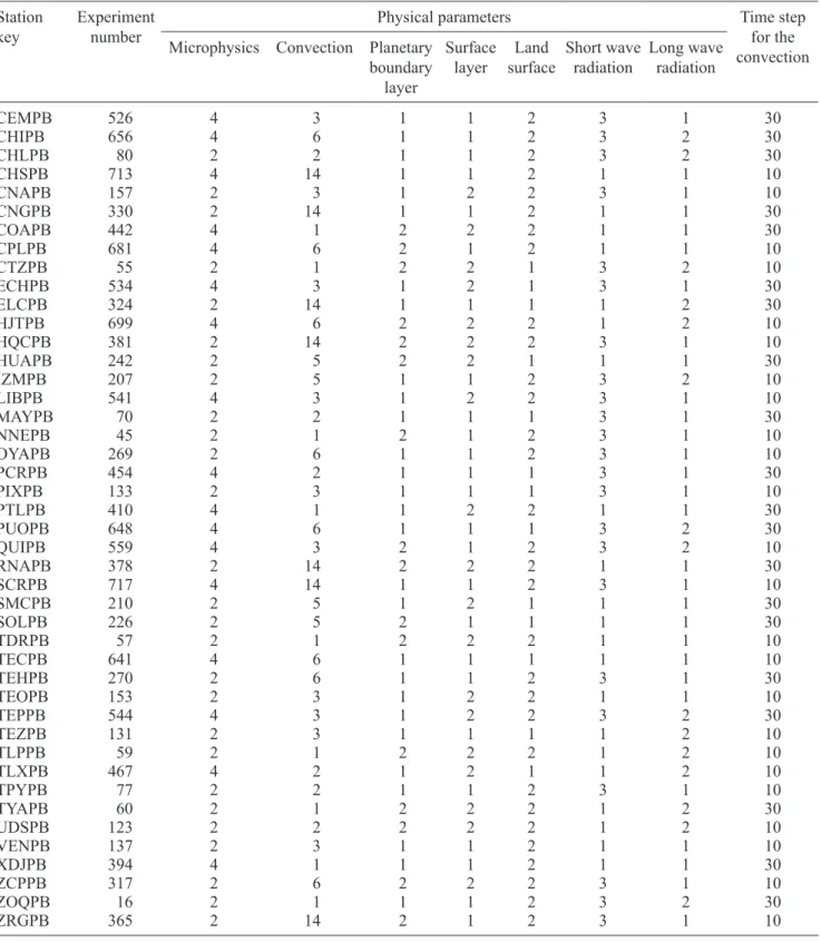
3.3. Optimal configuration of the WRF model

Three optimal configurations were determined to execute the WRF model by location, each one corre-sponding to the experiment which obtained the better performance in the three evaluation metrics. Tables VI, VII and VIII describe the optimal configurations according to the statistical parameters of bias, RMSE, and Pearson correlation, respectively.

The results show that no single experiment has the best performance for the WRF model in all the observation sites, nor in the three statistical metrics. Although some experiments with high performance in different metrics and observation sites were iden-tified, they were scarce.

(9)

Table IV. Minimum and maximum values in the 768 experiments by statistical metric and weather station.

Station key BIAS RMSE r

Minimun Maximum Minimun Maximum Minimun Maximum

ACHPB 0.01 1.16 3.18 13.52 0.07 0.85

ACJPB 0.01 1.89 5.70 34.74 0.21 0.67

ADOPB 6.89 5.15 7.95 22.09 0.12 0.68

AFRPB 3.77 5.26 9.85 29.51 0.06 0.52

AHAPB –0.01 3.53 6.94 28.74 0.16 0.79

AHUPB 0.02 3.12 4.71 20.51 0.17 0.92

APAPB –0.03 9.36 15.13 30.14 0.03 0.72

ATXPB 0.01 4.60 7.81 24.53 0.06 0.57

AVCPB 0.01 7.04 14.46 34.25 0.01 0.50

CDSPB –0.01 1.94 4.65 19.66 0.05 0.91

CEMPB –0.01 3.38 7.63 31.26 0.08 0.68

CHIPB –0.01 4.57 7.82 44.97 –0.02 0.49

CHLPB –0.01 7.06 9.11 27.29 0.12 0.61

CHSPB –0.01 5.19 10.59 24.47 –0.07 0.44

CNAPB 0.01 6.17 9.46 32.02 0.04 0.51

CNGPB –0.02 1.61 5.00 26.36 0.29 0.88

COAPB 0.01 5.64 10.86 29.90 0.00 0.87

CPLPB –0.15 2.92 6.28 31.48 0.15 0.62

CTZPB –0.02 10.73 21.31 43.26 –0.04 0.27

ECHPB –0.01 5.73 10.91 32.81 0.09 0.63

ELCPB –0.01 3.49 5.63 32.99 –0.01 0.88

HJTPB 0.01 4.72 7.18 20.78 0.08 0.62

HQCPB 0.03 5.50 8.28 41.70 0.09 0.68

HUAPB 0.02 6.42 9.68 32.22 0.05 0.82

IZMPB –0.01 4.91 7.87 39.48 –0.06 0.49

LIBPB 0.01 1.70 6.15 24.74 0.04 0.78

MAYPB –0.01 4.37 9.55 33.45 –0.03 0.52

NNEPB –0.01 6.82 10.88 42.27 –0.06 0.71

OYAPB 0.03 0.50 6.69 37.95 –0.06 0.98

PCRPB 0.02 3.10 7.77 35.20 –0.05 0.71

PIXPB 0.01 2.79 6.96 30.98 –0.04 0.60

PTLPB –0.01 10.22 12.84 31.63 0.07 0.68

PUOPB 0.01 5.94 10.49 33.13 0.10 0.57

QUIPB –0.01 7.04 12.85 24.81 0.03 0.52

RNAPB 0.01 6.92 14.66 24.42 0.04 0.74

SCRPB –0.01 7.26 11.46 31.71 –0.02 0.56

SMCPB –0.01 2.57 6.60 27.81 –0.07 0.50

SOLPB –0.01 11.99 15.53 55.27 –0.07 0.86

TDRPB –0.01 12.06 16.93 39.78 –0.04 0.86

TECPB –0.01 1.09 5.58 28.05 –0.06 0.93

TEHPB 0.01 0.18 4.02 18.83 –0.07 0.49

TEOPB –0.01 5.16 7.91 25.87 –0.02 0.95

TEPPB 0.01 7.63 11.64 31.04 0.02 0.73

TEZPB –0.01 5.98 25.54 33.67 –0.08 0.06

TLPPB 0.01 18.06 28.00 34.46 –0.05 0.33

TLXPB 0.02 3.20 6.92 33.49 0.03 0.51

TPYPB 0.01 1.15 3.14 15.92 0.23 0.92

TYAPB –0.01 14.77 21.83 29.91 –0.10 0.36

UDSPB 0.01 7.23 10.58 41.61 0.05 0.77

(10)

Table V. Experiments with better performance by statistical metrics and weather station.

Group

number Station key Altitude

BIAS RMSE r

Experiment

number Value Experiment number Value Experiment number Value

1

AVCPB 240 223 0.01 141 14.46 141 0.50

RNAPB 360 378 0.01 589 14.66 269 0.74

TLPPB 300 59 6.89 538 28.00 538 0.33

TYAPB 100 60 3.77 597 21.83 259 0.36

2

CHIPB 929 656 –0.01 314 7.82 273 0.49

CHSPB 940 713 0.02 390 10.59 1 0.44

CTZPB 980 55 –0.03 747 21.31 747 0.27

PTLPB 525 410 0.01 341 12.84 341 0.68

3

ADOPB 1270 189 0.01 343 7.95 343 0.68

COAPB 1210 442 –0.01 279 10.86 279 0.87

HUAPB 1472 242 –0.01 318 9.68 277 0.82

IZMPB 1260 207 –0.01 718 7.87 192 0.49

NNEPB 1364 45 –0.01 334 10.88 140 0.71

PIXPB 1119 133 –0.01 626 6.96 565 0.60

TLXPB 1065 467 0.01 725 6.92 725 0.51

UDSPB 1472 123 –0.02 618 10.58 9 0.77

VENPB 1200 137 0.01 621 8.85 646 0.67

XDJPB 1180 394 –0.15 670 14.69 670 0.78

4

AHAPB 2000 533 –0.02 247 6.94 372 0.79

ATXPB 1855 696 –0.01 222 7.81 132 0.57

HQCPB 1580 381 –0.01 335 8.28 6 0.68

SOLPB 1590 226 0.01 373 15.53 124 0.86

TDRPB 1560 57 0.03 493 16.93 493 0.86

TEHPB 1648 270 0.02 393 4.02 397 0.49

TEOPB 1725 153 –0.01 766 7.91 766 0.95

TEPPB 1526 544 0.01 10 11.64 10 0.73

TEZPB 1950 131 –0.01 597 25.54 456 0.06

Table IV. Minimum and maximum values in the 768 experiments by statistical metric and weather station.

Station key BIAS RMSE r

Minimun Maximum Minimun Maximum Minimun Maximum

XDJPB 0.01 11.48 14.69 40.96 0.06 0.78

ZCPPB –0.01 3.73 8.25 69.73 –0.06 0.98

ZOQPB –0.01 6.47 13.73 30.46 –0.04 0.27

ZRGPB 0.01 3.54 8.75 41.73 –0.07 0.98

(11)

Table V. Experiments with better performance by statistical metrics and weather station.

Group

number Station key Altitude

BIAS RMSE r

Experiment

number Value Experiment number Value Experiment number Value

5

ACHPB 2340 697 –0.01 397 3.18 512 0.85

ACJPB 2330 693 0.03 398 5.70 717 0.67

AFRPB 2120 2 0.02 206 9.85 206 0.52

AHUPB 2216 235 0.01 622 4.71 256 0.92

CEMPB 2225 526 –0.01 739 7.63 264 0.68

CHLPB 2155 80 0.01 718 9.11 707 0.61

CNAPB 2150 157 –0.01 325 9.46 218 0.51

CNGPB 2300 330 0.01 638 5.00 37 0.88

CPLPB 2430 681 –0.01 325 6.28 135 0.62

ECHPB 2075 534 –0.01 214 10.91 263 0.63

ELCPB 2160 324 –0.01 323 5.63 339 0.88

HJTPB 2260 699 –0.01 53 7.18 452 0.62

LIBPB 2430 541 –0.01 650 6.15 278 0.78

MAYPB 2122 70 0.01 213 9.55 11 0.52

PUOPB 2179 648 –0.01 610 10.49 610 0.57

QUIPB 2070 559 0.01 224 12.85 204 0.52

TECPB 2030 641 –0.01 247 5.58 248 0.93

ZCPPB 2045 317 0.01 347 8.25 752 0.98

ZOQPB 2175 16 0.02 370 13.73 328 0.27

ZRGPB 2493 365 0.01 22 8.75 394 0.98

6

APAPB 2970 220 –0.01 356 15.13 752 0.72

CDSPB 2550 78 0.01 397 4.65 636 0.91

OYAPB 2850 269 –0.02 314 6.69 267 0.98

PCRPB 2600 454 0.01 586 7.77 517 0.71

SCRPB 2513 717 –0.01 309 11.46 21 0.56

SMCPB 2583 210 –0.01 470 6.60 3 0.50

TPYPB 2924 77 0.01 127 3.14 686 0.92

Mean 0.19 10.13 0.67

Table VI. Description of the optimal configuration of the WRF model by location according to the BIAS statistical parameter. Station

key Experiment number Physical parameters Time step for the

convection Microphysics Convection Planetary

boundary layer

Surface

layer surfaceLand Short wave radiation Long wave radiation

ACHPB 697 4 6 2 2 2 1 1 10

ACJPB 693 2 3 2 2 2 3 1 10

ADOPB 189 2 3 2 2 2 3 1 10

AFRPB 2 2 1 1 1 1 1 1 30

AHAPB 533 4 3 1 2 1 3 1 10

AHUPB 235 2 5 2 1 2 1 2 10

APAPB 220 2 5 1 2 2 1 2 30

ATXPB 696 4 6 2 2 1 3 2 30

AVCPB 223 2 5 1 2 2 3 2 10

(12)

Table VI. Description of the optimal configuration of the WRF model by location according to the BIAS statistical parameter. Station

key Experiment number Physical parameters Time step for the

boundary layer

Surface

CEMPB 526 4 3 1 1 2 3 1 30

CHIPB 656 4 6 1 1 2 3 2 30

CHLPB 80 2 2 1 1 2 3 2 30

CHSPB 713 4 14 1 1 2 1 1 10

CNAPB 157 2 3 1 2 2 3 1 10

CNGPB 330 2 14 1 1 2 1 1 30

COAPB 442 4 1 2 2 2 1 1 30

CPLPB 681 4 6 2 1 2 1 1 10

CTZPB 55 2 1 2 2 1 3 2 10

ECHPB 534 4 3 1 2 1 3 1 30

ELCPB 324 2 14 1 1 1 1 2 30

HJTPB 699 4 6 2 2 2 1 2 10

HQCPB 381 2 14 2 2 2 3 1 10

HUAPB 242 2 5 2 2 1 1 1 30

IZMPB 207 2 5 1 1 2 3 2 10

LIBPB 541 4 3 1 2 2 3 1 10

MAYPB 70 2 2 1 1 1 3 1 30

NNEPB 45 2 1 2 1 2 3 1 10

OYAPB 269 2 6 1 1 2 3 1 10

PCRPB 454 4 2 1 1 1 3 1 30

PIXPB 133 2 3 1 1 1 3 1 10

PTLPB 410 4 1 1 2 2 1 1 30

PUOPB 648 4 6 1 1 1 3 2 30

QUIPB 559 4 3 2 1 2 3 2 10

RNAPB 378 2 14 2 2 2 1 1 30

SCRPB 717 4 14 1 1 2 3 1 10

SMCPB 210 2 5 1 2 1 1 1 30

SOLPB 226 2 5 2 1 1 1 1 30

TDRPB 57 2 1 2 2 2 1 1 10

TECPB 641 4 6 1 1 1 1 1 10

TEHPB 270 2 6 1 1 2 3 1 30

TEOPB 153 2 3 1 2 2 1 1 10

TEPPB 544 4 3 1 2 2 3 2 30

TEZPB 131 2 3 1 1 1 1 2 10

TLPPB 59 2 1 2 2 2 1 2 10

TLXPB 467 4 2 1 2 1 1 2 10

TPYPB 77 2 2 1 1 2 3 1 10

TYAPB 60 2 1 2 2 2 1 2 30

UDSPB 123 2 2 2 2 2 1 2 10

VENPB 137 2 3 1 1 2 1 1 10

XDJPB 394 4 1 1 1 2 1 1 30

ZCPPB 317 2 6 2 2 2 3 1 10

ZOQPB 16 2 1 1 1 2 3 2 30

(13)

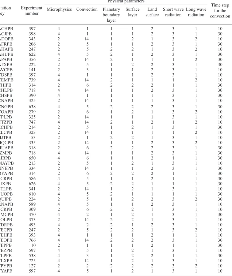
Table VII. Description of the optimal configuration of the WRF model by location according to the RMSE statistical parameter.

Station

key Experimentnumber

Physical parameters

Time step for the convection Microphysics Convection Planetary

boundary layer

Surface

ACHPB 397 4 1 1 1 2 3 1 10

ACJPB 398 4 1 1 1 2 3 1 30

ADOPB 343 2 14 1 2 1 3 2 10

AFRPB 206 2 5 1 1 2 3 1 30

AHAPB 247 2 5 2 2 1 3 2 10

AHUPB 622 4 5 2 1 2 3 1 30

APAPB 356 2 14 2 1 1 1 2 30

ATXPB 222 2 5 1 2 2 3 1 30

AVCPB 141 2 3 1 1 2 3 1 10

CDSPB 397 4 1 1 1 2 3 1 10

CEMPB 739 4 14 2 1 1 1 2 10

CHIPB 314 2 6 2 2 2 1 1 30

CHLPB 718 4 14 1 1 2 3 1 30

CHSPB 390 4 1 1 1 1 3 1 30

CNAPB 325 2 14 1 1 1 3 1 10

CNGPB 638 4 5 2 2 2 3 1 30

COAPB 279 2 6 1 2 1 3 2 10

CPLPB 325 2 14 1 1 1 3 1 10

CTZPB 747 4 14 2 1 2 1 2 10

ECHPB 214 2 5 1 2 1 3 1 30

ELCPB 323 2 14 1 1 1 1 2 10

HJTPB 53 2 1 2 2 1 3 1 10

HQCPB 335 2 14 1 1 2 3 2 10

HUAPB 318 2 6 2 2 2 3 1 30

IZMPB 718 4 14 1 1 2 3 1 30

LIBPB 650 4 6 1 1 2 1 1 30

MAYPB 213 2 5 1 2 1 3 1 10

NNEPB 334 2 14 1 1 2 3 1 30

OYAPB 314 2 6 2 2 2 1 1 30

PCRPB 586 4 5 1 1 2 1 1 30

PIXPB 626 4 5 2 2 1 1 1 30

PTLPB 341 2 14 1 2 1 3 1 10

PUOPB 610 4 5 2 1 1 1 1 30

QUIPB 224 2 5 1 2 2 3 2 30

RNAPB 589 4 5 1 1 2 3 1 10

SCRPB 309 2 6 2 2 1 3 1 10

SMCPB 470 4 2 1 2 1 3 1 30

SOLPB 373 2 14 2 2 1 3 1 10

TDRPB 493 4 2 2 1 2 3 1 10

TECPB 247 2 5 2 2 1 3 2 10

TEHPB 393 4 1 1 1 2 1 1 10

TEOPB 766 4 14 2 2 2 3 1 30

TEPPB 10 2 1 1 1 2 1 1 30

TEZPB 597 4 5 1 2 1 3 1 10

TLPPB 538 4 3 1 2 2 1 1 30

TLXPB 725 4 14 1 2 1 3 1 10

TPYPB 127 2 2 2 2 2 3 2 10

(14)

Table VII. Description of the optimal configuration of the WRF model by location according to the RMSE statistical parameter.

Station

Physical parameters

boundary layer

Surface

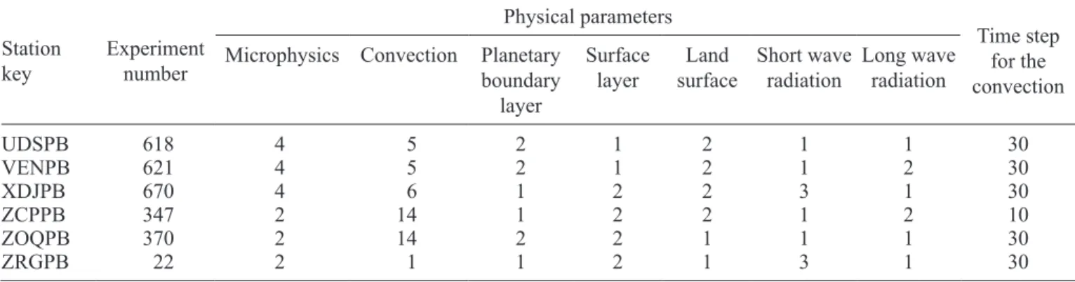
UDSPB 618 4 5 2 1 2 1 1 30

VENPB 621 4 5 2 1 2 1 2 30

XDJPB 670 4 6 1 2 2 3 1 30

ZCPPB 347 2 14 1 2 2 1 2 10

ZOQPB 370 2 14 2 2 1 1 1 30

ZRGPB 22 2 1 1 2 1 3 1 30

Table VIII. Description of the optimal configuration of the WRF model by location according to the Pearson correlation statistical parameter.

Station

Physical parameters

boundary layer

Surface

ACHPB 512 4 2 2 2 2 3 2 30

ACJPB 717 4 14 1 1 2 3 1 10

ADOPB 343 2 14 1 2 1 3 2 10

AFRPB 206 2 5 1 1 2 3 1 30

AHAPB 372 2 14 2 2 1 1 2 30

AHUPB 256 2 5 2 2 2 3 2 30

APAPB 752 4 14 2 1 2 3 2 30

ATXPB 132 2 3 1 1 1 1 2 30

AVCPB 141 2 3 1 1 2 3 1 10

CDSPB 636 4 5 2 2 2 1 2 30

CEMPB 264 2 6 1 1 1 3 2 30

CHIPB 273 2 6 1 2 1 1 1 10

CHLPB 707 4 14 1 1 1 1 2 10

CHSPB 1 2 1 1 1 1 1 1 10

CNAPB 218 2 5 1 2 2 1 1 30

CNGPB 37 2 1 2 1 1 3 1 10

COAPB 279 2 6 1 2 1 3 2 10

CPLPB 135 2 3 1 1 1 3 2 10

CTZPB 747 4 14 2 1 2 1 2 10

ECHPB 263 2 6 1 1 1 3 2 10

ELCPB 339 2 14 1 2 1 1 2 10

HJTPB 452 4 2 1 1 1 1 2 30

HQCPB 6 2 1 1 1 1 3 1 30

HUAPB 277 2 6 1 2 1 3 1 10

IZMPB 192 2 3 2 2 2 3 2 30

LIBPB 278 2 6 1 2 1 3 1 30

MAYPB 11 2 1 1 1 2 1 2 10

NNEPB 140 2 3 1 1 2 1 2 30

OYAPB 267 2 6 1 1 2 1 2 10

PCRPB 517 4 3 1 1 1 3 1 10

(15)

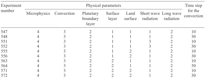
to the EMI (Table X), it was identified that the settings of the microphysics WRF Single-Moment (WSM) 5-class scheme (option 4), the convection parame-terization Grell-Devenyi ensemble scheme (option 3), the planetary boundary layer parameterization Mellor-Yamada-Janjic (Eta) TKE scheme (option 2), and the long wave radiation Goddard Shortwave Scheme (option 2) are kept constant to achieve a comparable performance at the state level.

Figures 2-8 present the time series correspond-ing to observed precipitation in comparison to simulated precipitation by the WRF model, which were analyzed in four experiments corresponding to the following parameters: (1) less BIAS, (2) lower RMSE, (3) greater Pearson correlation, and (4) higher statewide EMI. The following four observations were derived from this time series analysis:

During the study period, the state of Puebla pre-sented a strong rainfall concentration (greater than

25 mm per day) from June 20 to July 10. Intense to extraordinary rainfall (greater than 75 mm per day) also took place at 23 observation sites in the northern part of the state due to Hurricane Franklin on Au-gust 10, exceeding the highest historical rainfall at SOLPB, ZCPPB, and ZRGPB stations with records of 225, 281 and 198 mm, respectively.

It was observed that in the CTZPB station, the observed data of extraordinary rainfall occurred on August 10 show a two-days forward displacement, while at the TEZPB station data show a one-day backward change . Therefore, there might be an error in the capture dates at these two observation sites, which would explain the poor performance of the WRF model at these locations.

Although the three best experiments identified by location (corresponding to the lower bias and RMSE, and the higher Pearson correlation) show an outstanding performance of the WRF model in Table VIII. Description of the optimal configuration of the WRF model by location according to the Pearson correlation statistical parameter.

Station

Physical parameters

boundary layer

Surface

PTLPB 341 2 14 1 2 1 3 1 10

PUOPB 610 4 5 2 1 1 1 1 30

QUIPB 204 2 5 1 1 2 1 2 30

RNAPB 269 2 6 1 1 2 3 1 10

SCRPB 21 2 1 1 2 1 3 1 10

SMCPB 3 2 1 1 1 1 1 2 10

SOLPB 124 2 2 2 2 2 1 2 30

TDRPB 493 4 2 2 1 2 3 1 10

TECPB 248 2 5 2 2 1 3 2 30

TEHPB 397 4 1 1 1 2 3 1 10

TEOPB 766 4 14 2 2 2 3 1 30

TEPPB 10 2 1 1 1 2 1 1 30

TEZPB 456 4 2 1 1 1 3 2 30

TLPPB 538 4 3 1 2 2 1 1 30

TLXPB 725 4 14 1 2 1 3 1 10

TPYPB 686 4 6 2 1 2 3 1 30

TYAPB 259 2 6 1 1 1 1 2 10

UDSPB 9 2 1 1 1 2 1 1 10

VENPB 646 4 6 1 1 1 3 1 30

XDJPB 670 4 6 1 2 2 3 1 30

ZCPPB 752 4 14 2 1 2 3 2 30

ZOQPB 328 2 14 1 1 1 3 2 30

(16)

the precipitation simulation, they do not display the same performance in a homogeneous way in the 54 observation sites.

The performance of experiment 571, with the highest EMI at the state level in the 54 observation sites, is comparable to that obtained in the experi-ments that presented better performance locally for the bias, RMSE and r parameters.

Finally, Figure 9 shows the spatial distribution of the observed and simulated precipitation in experi-ment 571, together with its corresponding anomaly

for August 9, 10 and 11, 2017. On day 10, the highest rainfall of the study period occurred in the north-ern region of the state of Puebla, associated with Hurricane Franklin. It was observed that the WRF model had the ability to simulate the intensity of pre-cipitation during the extreme event; however, rainfall patterns show variations in detail. These variations are mainly associated with the fact that the 8-km resolution of the model in the nested domain was insufficient to characterize the terrain in the complex topography of the state.

Table IX. Statistical parameters of the 10 experiments with the best EMI at the state level. Experiment

number EMI _{Minimum Maximum Average Minimum Maximum Average Minimum Maximum Average}BIAS RMSE r

571 0.76 –0.62 10.59 9.27 9.74 42.32 24.98 0.06 0.77 0.35

555 0.75 –0.23 10.13 8.46 9.24 48.36 24.24 0.05 0.82 0.34

547 0.74 0.27 10.49 8.92 9.19 48.68 24.50 0.07 0.75 0.35

548 0.74 –0.36 10.70 9.13 11.22 46.69 24.83 0.06 0.79 0.36

572 0.73 –0.05 9.69 9.00 10.50 39.68 24.05 0.06 0.83 0.36

551 0.72 –0.23 11.86 6.66 9.20 39.10 22.39 0.07 0.72 0.37

556 0.72 0.11 8.44 8.63 10.05 42.50 23.81 0.04 0.86 0.36

563 0.71 –0.29 13.73 6.80 7.66 37.99 22.43 0.05 0.82 0.38

564 0.71 –0.26 13.50 6.74 7.71 32.46 21.80 0.04 0.81 0.37

552 0.70 0.97 11.33 6.83 10.92 37.73 21.86 0.08 0.82 0.39

Note: experiments were ordered from highest to lowest EMI.

Table X. Parameter configuration of the cases exposed with better EMI at the state level. Experiment

number Physical parameters Time step for the

boundary layer

Surface

547 4 3 2 1 1 1 2 10

548 4 3 2 1 1 1 2 30

551 4 3 2 1 1 3 2 10

552 4 3 2 1 1 3 2 30

555 4 3 2 1 2 1 2 10

556 4 3 2 1 2 1 2 30

563 4 3 2 2 1 1 2 10

564 4 3 2 2 1 1 2 30

571 4 3 2 2 2 1 2 10

572 4 3 2 2 2 1 2 30

(17)

200 Observed rain_{Lower BIAS (exp. 697)} Lower RMSE (exp. 141) Higher r (exp. 141) Higher EMI (exp. 571) 175 150 125 100 mm 75 50 25 0

10 20 30 40

Day 50 60 70 80 200 175 150 125 100 mm 75 50 25 0

10 20 30 40

Day 50 60 70 80

200 175 150 125 100 mm 75 50 25 0

10 20 30 40

Day 50 60 70 80 200 175 150 125 100 mm 75 50 25 0

10 20 30 40

Day 50 60 70 80

200 175 150 125 100 mm 75 50 25 0

10 20 30 40

Day 50 60 70 80 200 175 150 125 100 mm 75 50 25 0

10 20 30 40

Day 50 60 70 80

200 175 150 125 100 mm 75 50 25 0

10 20 30 40

Day 50 60 70 80 200 175 150 125 100 mm 75 50 25 0

10 20 30 40

Day 50 60 70 80

ACHPB ACJPB

Observed rain Lower BIAS (exp. 697) Lower RMSE (exp. 141) Higher r (exp. 141) Higher EMI (exp. 571)

ADOPB AFRPB

AHAPB AHUPB

APAPB ATXPB

(18)

AVCPB CDSPB CHLPB CHSPB CNAPB CNGPB CEMPB CHIPB 200 175 150 125 100 mm 75 50 25 0

10 20 30 40

Day 50 60 70 80

200 175 150 125 100 mm 75 50 25 0

10 20 30 40

Day 50 60 70 80

200 175 150 125 100 mm 75 50 25 0

10 20 30 40

Day 50 60 70 80 200 175 150 125 100 mm 75 50 25 0

10 20 30 40

Day 50 60 70 80

200 175 150 125 100 mm 75 50 25 0

10 20 30 40

Day 50 60 70 80 200 175 150 125 100 mm 75 50 25 0

10 20 30 40

Day 50 60 70 80 200 175 150 125 100 mm 75 50 25 0

10 20 30 40

Day 50 60 70 80 200 175 150 125 100 mm 75 50 25 0

10 20 30 40

Day 50 60 70 80 Observed rain

Lower BIAS (exp. 533) Lower RMSE (exp. 314) Higher r (exp. 273) Higher EMI (exp. 571)

(19)

COAPB CPLPB CTZPB ECHPB ELCPB HJTPB HQCPB HUAPB 200 175 150 125 100 mm 75 50 25 0

10 20 30 40

Day 50 60 70 80 200 175 150 125 100 mm 75 50 25 0

10 20 30 40

Day 50 60 70 80

200 175 150 125 100 mm 75 50 25 0

10 20 30 40

Day 50 60 70 80 200 175 150 125 100 mm 75 50 25

10 20 30 40

Day 50 60 70 80

200 175 150 125 100 mm 75 50 25 0

10 20 30 40

Day 50 60 70 80 200 175 150 125 100 mm 75 50 25 0

10 20 30 40

Day 50 60 70 80

200 175 150 125 100 mm 75 50 25 0

10 20 30 40

Day 50 60 70 80 200 175 150 125 100 mm 75 50 25 0

10 20 30 40

Day 50 60 70 80 Observed rain

(20)

IZMPB LIBPB MAYPB NNEPB OYAPB PCRPB PIXPB PTLPB 200 175 150 125 100 mm 75 50 25 0

10 20 30 40

Day 50 60 70 80 10 20 30 40Day 50 60 70 80

200 175 150 125 100 mm 75 50 25 0

10 20 30 40

Day 50 60 70 80 10 20 30 40Day 50 60 70 80

200 175 150 125 100 mm 75 50 25 0

10 20 30 40

Day 50 60 70 80 10 20 30 40Day 50 60 70 80

200 175 150 125 100 mm 75 50 25 0 200 175 150 125 100 mm 75 50 25 0 200 175 150 125 100 mm 75 50 25 0 200 175 150 125 100 mm 75 50 25 0 200 175 150 125 100 mm 75 50 25 0 10 20 30 40

Day 50 60 70 80 10 20 30 40Day 50 60 70 80 Observed rain

(21)

PUOPB QUIPB RNAPB SCRPB SMCPB SOLPB TDRPB TECPB 200 175 150 125 100 mm 75 50 25 0

10 20 30 40

Day 50 60 70 80 10 20 30 40Day 50 60 70 80

200 175 150 125 100 mm 75 50 25 0

10 20 30 40

Day 50 60 70 80 10 20 30 40Day 50 60 70 80

200 175 150 125 100 mm 75 50 25 0

10 20 30 40

Day 50 60 70 80 10 20 30 40Day 50 60 70 80

200 175 150 125 100 mm 75 50 25 0 200 175 150 125 100 mm 75 50 25 0 200 175 150 125 100 mm 75 50 25 200 175 150 125 100 mm 75 50 25 200 175 150 125 100 mm 75 50 25 0 10 20 30 40

Day 50 60 70 80 10 20 30 40Day 50 60 70 80 Observed rain

(22)

200 175 150 125 100 mm 75 50 25 0

10 20 30 40

Day 50 60 70 80 10 20 30 40Day 50 60 70 80

200 175 150 125 100 mm 75 50 25 0

10 20 30 40

Day 50 60 70 80 10 20 30 40Day 50 60 70 80

200 175 150 125 100 mm 75 50 25 0

10 20 30 40

Day 50 60 70 80 10 20 30 40Day 50 60 70 80

200 175 150 125 100 mm 75 50 25 0 200 175 150 125 100 mm 75 50 25 0 200 175 150 125 100 mm 75 50 25 200 175 150 125 100 mm 75 50 25 200 175 150 125 100 mm 75 50 25 0 10 20 30 40

Day 50 60 70 80 10 20 30 40Day 50 60 70 80

TEHPB TEOPB

TEPPB TEZPB

TLPPB TLXPB

TPYPB TYAPB

(23)

4. Discussion

The performance of the mesoscale models is sensitive to physical parameterization schemes, so it is nec-essary to perform several experiments with different combinations (Das et al., 2015). In this context, the relevance of evaluating the WRF model with different physical settings for the state of Puebla is evident, especially before the possible implementation of the model in an operational way for the issuance of

mete-orological alerts, the implementation of early warning systems, or the undertaking of studies. Otherwise there is a risk of obtaining values that do not repre-sent the real or approximate precipitation behavior, and significant errors in the forecast will hinder the prevention and analysis of natural disasters.

In correspondence with the works of Ochoa et al. (2015) and Wu et al. (2016), it is highlighted that the WRF model can reproduce individual peaks of

TEHPB TEOPB

TEPPB TEZPB

TLPPB TLXPB

200 175 150 125 100

mm

75 50 25 0

10 20 30 40

Day 50 60 70 80 10 20 30 40Day 50 60 70 80

200 175 150 125 100

mm

75 50 25 0

10 20 30 40

Day 50 60 70 80 10 20 30 40Day 50 60 70 80

200 175 150 125 100

mm

75 50 25 0

10 20 30 40

Day 50 60 70 80 10 20 30 40Day 50 60 70 80 200

175 150 125 100

mm

75 50 25

200 175 150 125 100

mm

75 50 25

200 175 150 125 100

mm

75 50 25 Observed rain

(24)

Fig. 9. Spatial distribution of rainfall on August 9-11, 2017. Left: observed rainfall; center: rainfall simulated with the WRF model in experiment 571; right: anomaly between observed rainfall and rainfall simulated in experiment 571.

Observed rain (2017/08/09)

0 10 20 30 40

mm 50 60 70 80 0 10 20 30 40mm 50 60 70 80 mm

0 20 40 60 80

mm 100 120 160

–60 –40 –20 0 20 40 60

mm

–60 –40 –20 0 20 40 60

mm

–60 –40 –20 0 20 40 60 Rain forecast in experiment 571 (2017/08/09) Rain anomaly (2017/08/09)

0 10 20 30 40

mm 50 60 70 80 0 10 20 30 40mm 50 60 70 80

Observed rain (2017/08/10) Rain forecast in experiment 571 (2017/08/10) Rain anomaly (2017/08/10)

Observed rain (2017/08/11) Rain forecast in experiment 571 (2017/08/11) Rain anomaly (2017/08/11) 140

0 20 40 60 80

(25)

precipitation, thus allowing to analyze the evolution of intense precipitation events in the study area, such as those observed on August 10 in the north region of the state of Puebla, originated by the passage of Hurricane Franklin. On the other hand, Lekhadiya and Jana (2018) mention that the WRF model can very well represent the cloud pattern and spatially recognizes rain events, but that it overestimates the determination in the six parameterization schemes evaluated in their study.

The results in this study point out that the WRF model has the capacity to achieve a high performance for precipitation forecast in specific locations in the state of Puebla, attaining very high positive cor-relations with values of up to 0.98 at the OYAPB, ZCPPB, and ZRGPB stations, a limited significant cumulative bias of ± 0.01 in 41 of the observation sites (76%), and a low intensity RMSE with values below 3.18 mm at ACHPB and TPYPB stations. However, the optimal configuration of the model in one location does not offer the same level of perfor-mance in other observation sites. This result corre-sponds to Jankov and Gallus (2005), who evaluated the impact of 18 different combinations of physical settings and their interaction with the precipitation of mesoscale convective systems, concluding that none of the scores obtained with the evaluation metrics applied (correspondence relationship and squared correlation coefficient) in the18 combinations was the best for all times and thresholds. However, in this study, by selecting experiment 571, which obtained the highest EMI value, it was shown that it is possible to obtain acceptable results at the state level.

5. Conclusions

In compliance with the first objective of this work, the results of the quantitative evaluation of the WRF model performance for simulating rainfall in the state of Puebla, allowed us to determine that it is possible to configure the model to obtain high performance per observation site and acceptable performance statewide.

Of the 54 observation sites, only the TEZPB station had unsatisfactory results with respect to the Pearson correlation, which obtained a maximum of 0.06 in experiment 456, and a high RMSE with a value of 25.54 in experiment 597. However, for this

location, an acceptable bias was obtained with a value of –0.01 in experiment 131.

The application of the Efficiency Multiparameter Index allowed the determination of experiment 571 as the optimal configuration of the WRF model for a statewide application. In addition, after analyzing the 10 best configurations according to the EMI, it was identified that the settings of the microphysics WRF Single-Moment (WSM) 5-class scheme (option 4), the convection parameterization Grell-Devenyi ensemble scheme (option 3), the planetary boundary layer parameterization Mellor-Yamada-Janjic (Eta) TKE scheme (option 2), and the long wave radia-tion Goddard Shortwave Scheme (opradia-tion 2), should remain constant to achieve acceptable and uniform performance at the state level.

It should be noted that, in general, the WRF model has a better performance at altitudes greater than 2000 masl, especially in the northern and central regions of the state of Puebla, while in latitudes below 1000 masl, mainly in the south and southeast regions of the state, the model performance is below the state average.

(26)

Additionally, the differentiated signal between bias and RMSE in the best experiments for each observation site, indicates that in the simulation of precipitation in the state of Puebla, the WRF model does not present systematic errors that can be adjusted directly by linear regression. That is, the errors occur randomly, associated with the chaotic behavior of the atmosphere.

Finally, as future work, it is proposed to apply the methodology presented in this research to calibrate the WRF model at the national level.

References

Aguilar C. 1997. Simulación de sistemas, aplicaciones en producción animal. Colección en Agricultura. Pontificia Universidad Católica de Chile, Facultad de Agronomía, Santiago, Chile.

Anderson DR, Sweeney DJ, Williams TA. 2008. Estadísti-ca para administración y economía. 10a ed. Cengage Learning, México, 1056 p.

Arreguín-Cortés FI, López-Pérez M, Rodríguez-López O, Montero-Martínez MJ (coords.). 2015. Atlas de vulner-abilidad hídrica en México ante el cambio climático: efectos del cambio climático en el recurso hídrico de México. Instituto Mexicano de Tecnología del Agua, Jiutepec, México.

Aparicio J. 1998. Inundaciones: la otra cara de la moneda. Revista Tláloc, órgano informativo de la Asociación Mexicana de Hidráulica 5(11), 15-20.

Babbie ER. 2014. The basics of social research. Wadsworth Cengage Learning, Belmont, CA.

Barrales L, Peña I, Fernández P. 2004. Validación de modelos: un enfoque aplicado. Agricultura Técnica 64(1), 66-73.

Benjamin MA. 2008. Analysing urban flood risk in low-cost settlements of George, Western Cape, South Africa: Investigating physical and social dimensions. M.Sc. Thesis. University of Cape Town, Cape Town, South Africa.

Campbell DT, Stanley JC. 2012. Diseños experimentales y cuasiexperimentales en la investigación social. 2a ed. Amorrortu, España.

Carbonell Turtos L, Capote Mastrapa G, Fonseca Ro-dríguez Y, Álvarez Escudero L, Sánchez Gacita M, Bezanilla Morlot A, Borrajero Montejo I, Meneses Ruiz E, Pire Rivas S. 2003. Assessment of the Weather Research and Forecasting model implementation in Cuba addressed to diagnostic air quality modeling.

Atmospheric Pollution Research 4, 64-74. https://doi. org/10.5094/APR.2013.007

CONAGUA. 2017. Las lluvias que dejó #Franklin romp-ieron récords históricos en #Puebla. Comisión Nacional del Agua, 10 de agosto [tuit]. Available at: https://twit-ter.com/conagua_clima/status/895776809563734017 Creswell JW. 2013. Research design: Qualitative, quanti-tative, and mixed methods. Sage Publications, USA. Das MK, Chowdhury AM, Das S. 2015. Sensitivity study

with physical parameterization schemes for simulation of mesoscale convective systems associated with squall events. International Journal of Earth and Atmospheric Science 2, 20-36.

Douben KJ. 2006. Characteristics of river floods and flooding: A global overview, 1983-2003. Irrigation and Drainage 55, 9-21. https://doi.org/ https://doi. org/10.1002/ird.239

Gavidia M. 2012. Simulación de las variables meteorológi-cas en la ciudad de Lima para el verano e invierno de 2009 con el modelo Weather Research and Forecast-ing. Bachelor thesis in Environmental EngineerForecast-ing. Universidad Nacional Agraria La Molina, Lima, Perú. Henríquez-Fierro E, Zepeda-González MI. 2003. Prepa-ración de un proyecto de investigación. Ciencia y Enfermería 9, 23-28. https://doi.org/10.4067/S0717-95532003000200003

Hernández-Sampeiri R, Fernández-Collado C, Baptis-ta-Lucio P. 2014. Metodología de la investigación. 6a ed. McGrawHill, México.

Hernández-Uribe RE, Barrios-Piña H, Ramírez AI. 2017. Análisis de riesgo por inundación: metodología y aplicación a la cuenca Atemajac. Tecnología y Cien-cias del Agua 8, 5-25. https://doi.org/10.24850/j-ty-ca-2017-03-01

Jankov I, Gallus WA. 2005. The impact of different WRF model physical parameterizations and their interactions on warm season MCS rainfall. Weather and Forecasting 20, 1048-1060. https://doi.org/10.1175/WAF888.1 Jáuregui E. 1989. Los ciclones del norte de México y sus

efectos sobre la precipitación. Ingeniería Hidráulica en México, septiembre-diciembre.

Kalnay E. 2003. Atmospheric modeling, data assimilation, and predictability. Cambridge University Press, New York, USA.

(27)

Mitchell PL. 1997. Misuse of regression for empirical validation of models. Agricultural Systems 54, 313-326. https://doi.org/10.1016/S0308-521X(96)00077-7 Mondragón-Barrera MA. 2014. Uso de la correlación de

Spearman en un estudio de intervención en fisiotera-pia. Movimiento científico 8(1), 98-104. https://doi. org/10.33881/2011-7191.mct.08111

Moya-Álvarez AS, Ortega-León JM. 2015. Aplicación del modelo meteorológico WRF para el pronóstico de precipitaciones en período lluvioso de Cuba, 2014. Apuntes de Ciencia & Sociedad 5, 135-145. https:// doi.org/10.18259/acs.2015021

Moya de Madrigal L. 2005. Introducción a la estadística de la salud. 6a ed. Universidad de Costa Rica, Costa Rica, 330 pp.

Ochoa CA, Quintanar AI, Raga GB, Baumgardner D. 2015. Changes in intense precipitation events in Mexico City. Journal of Hydrometeorology 16, 1804-1820. https:// doi.org/10.1175/JHM-D-14-0081.1

Pielke RA. 1984. Mesoscale meteorological modeling. Academic Press, Orlando, FL.

Rauscher HM, Young MJ, Webb CD, Rohison DJ. 2000. Testing the accuracy of growth and yields models for Southern hardwood forests. Southern Journal of Applied Forestry 24(3), 176-185.

Reynolds MR. 1984. Estimating the error in model predictions. Forest Science 30, 454-469. https://doi. org/10.1093/forestscience/30.2.454

SEGOB. 2009. Características e impacto socioeconómico de los principales desastres ocurridos en la República

Mexicana en el año 2008. Centro Nacional de Pre-vención de Desastres, Secretaria de Gobernación, México.

Skamarock WC, Klemp JB, Dudhia J, Gill DO, Barker DM, Huang X-Y, Wang W, Powers JG. 2008. De-scription of the Advanced Research WRF version 3. National Center for Atmospheric Research, Boulder, Colorado, USA. https://doi.org/10.5065/ D68S4MVH

Tamayo JL. 1996. Geografía moderna de México. Trillas, México.

White TL, McBurney DH. 2013. Research methods. Cen-gage Learning, USA, 458 pp.

Wu D, Peters-Lidard C, Tao WK, Petersen W. 2016. Evaluation of NU-WRF rainfall forecasts for IFloodS. Journal of Hidrometeorology 17, 1317-1335. https:// doi.org/10.1175/JHM-D-15-0134.1

Zepka GS. 2011. Previsão de descargas atmosféricas usando o modelo de mesoescala WRF. Ph.D. Thesis in Space Geophysics. Instituto Nacional de Pesquisas Espaciais, São José dos Campos, Brasil.

Willmott CJ. 1982. Some comments on the evaluation of model performance. Bulletin of the American Meteo-rological Society 63, 1309-1313. https://doi.org/10.1 175/1520-0477(1982)063<1309:SCOTEO>2.0.CO;2 Willmott C, Ackleson S, Davis R, Feddema J, Klink K,