Comparing approximate methods for mock catalogues and
covariance matrices I: correlation function
Martha Lippich
1
,
2
,
?
Ariel G. S´
anchez
2
, Manuel Colavincenzo
3
,
4
,
5
,
Emiliano Sefusatti
6
,
7
, Pierluigi Monaco
5
,
6
,
7
, Linda Blot
8
,
9
, Martin Crocce
8
,
9
,
Marcelo A. Alvarez
10
, Aniket Agrawal
11
, Santiago Avila
12
,
Andr´
es Balaguera-Antol´ınez
13
,
14
, Richard Bond
15
, Sandrine Codis
15
,
16
,
Claudio Dalla Vecchia
13
,
14
, Antonio Dorta
13
,
14
, Pablo Fosalba
8
,
9
,
Albert Izard
17
,
18
,
8
,
9
, Francisco-Shu Kitaura
13
,
14
, Marcos Pellejero-Ibanez
13
,
14
,
George Stein
15
, Mohammadjavad Vakili
19
, Gustavo Yepes
20
,
21
1 Universit¨ats-Sternwarte M¨unchen, Ludwig-Maximilians-Universit¨at M¨unchen, Scheinerstrasse 1, 81679 Munich, Germany
2 Max-Planck-Institut f¨ur extraterrestrische Physik, Postfach 1312, Giessenbachstr., 85741 Garching, Germany
3 Dipartimento di Fisica, Universit`a di Torino, Via P. Giuria 1, 10125 Torino, Italy
4 Istituto Nazionale di Fisica Nucleare, Sezione di Torino, Via P. Giuria 1, 10125 Torino, Italy
5 Dipartimento di Fisica, Sezione di Astronomia, Universit`a di Trieste, via Tiepolo 11, 34143 Trieste, Italy
6 Istituto Nazionale di Astrofisica, Osservatorio Astronomico di Trieste, via Tiepolo 11, 34143 Trieste, Italy
7 Istituto Nazionale di Fisica Nucleare, Sezione di Trieste, Via Valerio, 2, I-34127 Trieste, Italy
8 Institute of Space Sciences (ICE, CSIC), Campus UAB, Carrer de Can Magrans, s/n, 08193 Barcelona, Spain
9 Institut d’Estudis Espacials de Catalunya (IEEC), 08193 Barcelona, Spain
10Berkeley Center for Cosmological Physics, Campbell Hall 341, University of California, Berkeley CA 94720
11Max-Planck-Institut f¨ur Astrophysik, Karl-Schwarzschild-Str. 1, 85741 Garching, Germany
12Institute of Cosmology & Gravitation, Dennis Sciama Building, University of Portsmouth, Portsmouth PO1 3FX, UK
13Instituto de Astrof´ısica de Canarias, C/V´ıa L´actea, s/n, E-38200, La Laguna, Tenerife, Spain
14Departamento Astrof´ısica, Universidad de La Laguna, E-38206 La Laguna, Tenerife, Spain
15Canadian Institute for Theoretical Astrophysics, University of Toronto, 60 St. George Street, Toronto, ON M5S 3H8, Canada
16Institut d’Astrophysique de Paris, CNRS & Sorbonne Universit´e, UMR 7095, 98 bis boulevard Arago, 75014 Paris, France
17Jet Propulsion Laboratory, California Institute of Technology, 4800 Oak Grove Drive, Pasadena, CA 91109, USA
18Department of Physics and Astronomy, University of California, Riverside, CA 92521, USA
19Leiden Observatory, Leiden University, P.O. Box 9513, NL-2300 RA, Leiden, The Netherlands
20Departamento de F´ısica Te´orica, M´odulo 15, Universidad Aut´onoma de Madrid, 28049 Madrid, Spain
21Centro de Investigaci´on Avanzada en F´ısica Fundamental (CIAFF), Universidad Aut´onoma de Madrid, 28049, Madrid, Spain
Accepted XXX. Received YYY; in original form ZZZ
ABSTRACT
This paper is the first in a set that analyses the covariance matrices of clustering statis-tics obtained from several approximate methods for gravitational structure formation. We focus here on the covariance matrices of anisotropic two-point correlation func-tion measurements. Our comparison includes seven approximate methods, which can be divided into three categories: predictive methods that follow the evolution of the linear density field deterministically (ICE-COLA, Peak Patch, and Pinocchio), methods that require a calibration with N-body simulations (PatchyandHalogen), and simpler recipes based on assumptions regarding the shape of the probability dis-tribution function (PDF) of density fluctuations (log-normal and Gaussian density fields). We analyse the impact of using covariance estimates obtained from these ap-proximate methods on cosmological analyses of galaxy clustering measurements, using as a reference the covariances inferred from a set of full N-body simulations. We find that all approximate methods can accurately recover the mean parameter values
in-? [email protected]
ferred using the N-body covariances. The obtained parameter uncertainties typically agree with the corresponding N-body results within 5% for our lower mass threshold, and 10% for our higher mass threshold. Furthermore, we find that the constraints for some methods can differ by up to 20% depending on whether the halo samples used to define the covariance matrices are defined by matching the mass, number density, or clustering amplitude of the parent N-body samples. The results of our configuration-space analysis indicate that most approximate methods provide similar results, with no single method clearly outperforming the others.
Key words: cosmological simulations – galaxies clustering – error estimation – large-scale structure of Universe
1 INTRODUCTION
The statistical analysis of the large-scale structure (LSS) of the Universe is one of the primary tools of observational cosmology. The analysis of the signature of baryon acoustic oscillations (BAO) and redshift-space distortions (RSD) on anisotropic two-point clustering measurements can be used to infer constraints on the expansion history of the Universe (Blake & Glazebrook 2003; Linder 2003) and the redshift evolution of the growth-rate of cosmic structures (Guzzo et al. 2008). Thanks to this information, LSS observations have shaped our current understanding of some of the most challenging open problems in cosmology, such as the nature of dark energy, the behaviour of gravity on large scales, and the physics of inflation (e.g. Efstathiou et al. 2002; Eisen-stein et al. 2005;Cole et al. 2005;S´anchez et al. 2006,2012; Anderson et al. 2012,2014a,b;Alam et al. 2017).
Future galaxy surveys such as Euclid (Laureijs et al. 2011) or the Dark Energy Spectroscopic Instrument (DESI) Survey (DESI Collaboration et al. 2016) will contain millions of galaxies covering large cosmological volumes. The small statistical uncertainties associated with clustering measure-ments based on these samples will push the precision of our tests of the standard ΛCDM scenario even further. In this
context, it is essential to identify all components of the sys-tematic error budget affecting cosmological analyses based on these measurements, as well as to define strategies to control or mitigate them.
A key ingredient to extract cosmological information out of anisotropic clustering statistics is robust estimates of their covariance matrices. In most analyses, covariance ma-trices are computed from a set of mock catalogues designed to reproduce the properties of a given survey. Ideally, these mock catalogues should be based on N-body simulations, which can reproduce the impact of non-linear structure for-mation on the clustering properties of a sample with high accuracy. Due to the finite number of mock catalogues, the estimation of the covariance matrix is affected by statisti-cal errors and the resulting noise must be propagated into the final cosmological constraints (Taylor et al. 2013; Do-delson & Schneider 2013; Percival et al. 2014;Sellentin & Heavens 2016). Reaching the level of statistical precision needed for future surveys might require the generation of several thousands of mock catalogues. As N-body simula-tions are expensive in terms of run-time and memory, the construction of a large number of mock catalogues might be infeasible. The required number of realizations can be re-duced by means of methods such as resampling the phases
of N-body simulations (Hamilton et al. 2006;Schneider et al. 2011), shrinkage (Pope & Szapudi 2008), or covariance ta-pering (Paz & S´anchez 2015). However, even after applying such methods, the generation of multiple N-body simula-tions with the required number-density and volume to be used for the clustering analysis of future surveys would be extremely demanding.
During the last decades, several approximate methods for gravitational structure formation and evolution have been developed, which allow for a faster generation of mock catalogues; seeMonaco (2016) for a review. The accuracy with which these methods reproduce the covariance matri-ces estimated from N-body simulations must be thoroughly tested to avoid introducing systematic errors or biases on the parameter constraints derived from LSS measurements.
Colavincenzo et al.(2018) perform an analogous comparison based on power spectrum and bispectrum measurements.
The structure of the paper is as follows. Section 2 presents a brief description of the reference N-body simu-lations and the different approximate methods and recipes included in our comparison. In Section3we summarize the methodology used in this analysis, including a description of the halo samples that we consider (Section3.1), our cluster-ing measurements (Section 3.2), the estimation of the cor-responding covariance matrices (Section3.3), and the mod-elling for the correlation function used to asses the impact of the different methods when estimating parameter con-straints (Section3.4). We present a comparison of the clus-tering properties of the different halo samples in Section4.1 and their corresponding covariance matrices in Section4.2. In Section4.3we compare the performance of the different covariance matrices by analysing parameter constraints ob-tained from representative fits, using as a reference the ones obtained when the analysis is based on N-body simulations. We discuss the results from this comparison in Section 5. Finally, Section6presents our main conclusions.
2 APPROXIMATE METHODS FOR COVARIANCE MATRIX ESTIMATES
2.1 Methods included in the comparison
In this comparison project, we included covariance matrices inferred from different approximate methods and recipes, which we compared to the estimates obtained from a set of reference N-body simulations. Approximate methods have recently been revived by high-precision cosmology, due to the need of producing a large number of realizations to com-pute covariance matrices of clustering measurements. This topic has been reviewed byMonaco(2016), where methods have been roughly divided into two broad classes.
“Lagrangian” methods, as N-body simulations, are ap-plied to a grid of particles subject to a perturbation field. They reconstruct the Lagrangian patches that collapse into dark matter halos, and then displace them to their Eulerian positions at the output redshift, typically with Lagrangian Perturbation Theory (hereafter LPT). ICE-COLA, Peak Patch and Pinocchio fall in this class. These methods are predictive, in the sense that, after some cosmology-independent calibration of their free parameters (that can be thought at the same level as the linking length of friends-of-friends halo finders), they give their best reproduction of halo masses and clustering without any further tuning. This approach can be demanding in terms of computing resources and can have high memory requirements. In particular, ICE-COLAbelongs to the class of Particle-Mesh codes; these are in fact N-body codes that converge to the true solution (at least on large scales) for sufficiently small time-steps. As such, Particle-Mesh codes are expected to be more accurate than other approximate methods, at the expense of higher computational costs.
The second class of “bias-based” methods is based on the idea of creating a mildly non-linear density field using some version of LPT, and then populate the density field with halos that follow a given mass function and a speci-fied bias model. The parameters of the bias model must be
calibrated on a simulation, so as to reproduce halo cluster-ing as accurately as possible. The point of strength of these methods is their very low computational cost and memory requirement, that makes it possible to generate thousands of realizations in a simple workstation, and to push the mass limit to very low masses. This is however achieved at the cost of lower predictivity, and need of recalibration when the sample selection changes.HalogenandPatchyfall in this category.
In the following, we will refer to the two classes as “pre-dictive” and “calibrated” models. All approximate methods used here have been applied to the same set of 300 initial conditions (ICs) of the reference N-body simulations, so as to be subject to the same sample variance; as a consequence, the comparison, though limited to a relatively small number of realizations, is not affected by sample variance.
Additionally, we included in the comparison two simple recipes for the shape of the PDF of the density fluctuations, a Gaussian analytic model that is only valid in linear theory and a log-normal model. The latter was implemented by generating 1000 catalogues of “halos” that Poisson-sample a log-normal density field; in this test case we do not match the ICs with the reference simulations, and use a higher number of realizations to lower sample variance.
2.2 Reference N-body halo catalogue: Minerva
Our reference catalogues for the comparison of the differ-ent approximate methods is derived from a set of 300 N-body simulations called Minerva, which were performed us-ing GADGET-3 (last described in Springel 2005). To the first set of 100 realizations, which is described in more de-tail inGrieb et al.(2016) and was used in the recent BOSS analyses byS´anchez et al. (2017) and Grieb et al.(2017), 200 new independent realizations were added, which were generated with the same set-up as the first simulations. The initial conditions were derived from second-order La-grangian perturbation theory (2LPT) and use the cosmo-logical parameters that match the best-fitting results of the WMAP+BOSS DR9 analysis byS´anchez et al.(2013) at a starting redshiftzini=63. Each realization is a cubic box of side lengthLbox=1.5h−1Gpc with10003dark-matter (DM) particles and periodic boundary conditions. For the approx-imate methods described in the following sections we use the same box size and exactly the same ICs for each re-alization as in the Minerva simulations. Halos were identi-fied with a standard Friends-of-friends (FoF) algorithm at a snapshot of the simulations atz=1.0. FoF halos were then subject to the unbinding procedure provided by the SUB-FINDcode (Springel et al. 2001), where particles with posi-tive total energy are removed and halos that were artificially linked by FoF are separated. Given the particle mass reso-lution of the Minerva simulations, the minimum halo mass is2.667×1012h−1M.
2.3 Predictive methods
2.3.1 ICE-COLA
numerical integration. It starts by computing the initial con-ditions using second-order Lagrangian Perturbation Theory (2LPT, see Crocce et al. 2006). Then, it evolves particles along their 2LPT trajectories and adds a residual displace-ment with respect to the 2LPT path, which is integrated numerically using the N-body solver. Mathematically, the displacement fieldxis decomposed into the LPT component xLPT and the residual displacementxresas
xres(t)≡x(t)−xLPT(t). (1) In a dark matter-only simulation, the equation of motion relates the acceleration to the Newtonian potentialΦ, and
omitting some constants it can be written as: ∂t2x(t) =
−∇Φ(t). Using equation (1), the equation of motion reads
∂t2xres(t) =−∇Φ(t)−∂t2xLPT(t). (2)
COLA uses a Particle-Mesh method to compute the gra-dient of the potential at the position x (first term of the right hand side), it subtracts the acceleration correspond-ing to the LPT trajectory and finally the time derivatives on the left hand side are discretized and integrated numer-ically using few time steps. The 2LPT ensures convergence of the dynamics at large scales, where its solution is exact, and the numerical integration solves the dynamics at small non-linear scales. Halos can be correctly identified running a Friends-of-Friends (FoF) algorithm (Davis et al. 1985) on the dark matter density field, and halo masses, positions and velocities are recovered with accuracy enough to build mock halo catalogues.
ICE-COLA(Izard et al. 2016,2018) is a modification of the parallel version of COLA developed inKoda et al. (2016) that produces all-sky light cone catalogues on-the-fly. Izard et al. (2016) presented an optimal configuration for the production of accurate mock halo catalogues and Izard et al. (2018) explains the light cone production and the modelling of weak lensing observables.
Mock halo catalogues were produced withICE-COLA placing 30 time steps between an initial redshift of zi=19 and z=01 and forces were computed in a grid with a cell size 3 times smaller than the mean inter-particle separation distance. For the FoF algorithm, a linking length ofb=0.2 was used. Each simulation reached redshift 0 and used 200 cores for 20 minutes in the MareNostrum3 supercomputer at the Barcelona Supercomputing Center2, consuming a total
of 20 CPU khrs for the 300 realizations.
2.3.2 Peak Patch
From each of the 300 initial density field maps of the Minerva suite, we generate halo catalogues following the peak patch approach initially introduced by Bond & Myers(1996). In particular, we use a new massively parallel implementation of the peak patch algorithm to create efficient and accu-rate realizations of the positions and peculiar velocities of dark matter halos. The peak patch approach is essentially a Lagrangian space halo finder that associates halos with the largest regions that have just collapsed by a given time. The
1 The time steps were linearly distributed with the scale factor. 2 http:www.bsc.es.
pipeline can be separated into four subprocesses: (1) the generation of a random linear density field with the same phases and power spectrum as the Minerva simulations; (2) identification of collapsed regions using the homogeneous el-lipsoidal collapse approximation; (3) exclusion and merging of the collapsed regions in Lagrangian space; and (4) as-signment of displacements to these halos using second order Lagrangian perturbation theory.
The identification of collapsed regions is a key step of the algorithm. The determination of whether any given re-gion will have collapsed or not is made by approximating it as an homogeneous ellipsoid, the fate of which is deter-mined completely by the principal axes of the deformation tensor of the linear displacement field (i.e. the strain) av-eraged over the region. In principle, the process of finding these local mass peaks would involve measuring the strain at every point in space, smoothed on every scale. However, ex-perimentation has shown that equivalent results can be ob-tained by measuring the strain around density peaks found on a range of scales3. This is done by smoothing the field on a series of logarithmically spaced scales with a top-hat kernel, from a minimum radius ofRf,min=2alatt, wherealattis the lattice spacing, to a maximum radius ofRf,max=40 Mpc, with a ratio of 1.2. For each candidate peak, we then find the largest radius for which a homogeneous ellipsoid with the measured mean strain would collapse by the redshift of interest. If a candidate peak has no radius for which a ho-mogeneous ellipsoid with the measured strain would have collapsed, then that point is thrown out. Each candidate point is then stored as a peak patch at its location with its radius. We then proceed down through the filter bank to all scales and repeat this procedure for each scale, resulting in a list of peak patches which we refer to as the unmerged catalogue.
The next step is to account for exclusion, an essential step to avoid double counting of matter, since distinct halos should not overlap, by definition. We choose here to use binary exclusion (Bond & Myers 1996). Binary exclusion starts from a ranked list of candidate peak patches sorted by mass or, equivalently, Lagrangian peak patch radius. For each patch we consider every other less massive patch that overlaps it. If the smaller patch is outside of the larger one, then the radius of the two patches is reduced until they are just touching. If the center of the smaller patch is inside the large one, then that patch is removed from the list. This process is repeated until the least massive remaining patch is reached.
Finally, we move halos according to 2LPT using dis-placements computed at the scale of the halo.
This method is very fast: each realization ran typically in 97 seconds on 64 cores of the GPC supercomputer at the SciNet HPC Consortium in Toronto (1.72 hours in total) . It allows to get accurate – and fast – halo catalogues
out any calibration, achieving high precision on the mass function typically for masses above a few1013M.
2.3.3 Pinocchio
The PINpointing Orbit Crossing Collapsed HIerarchical Ob-jects (Pinocchio) code (Monaco et al. 2002) is based on the following algorithm.
A linear density contrast field is generated in Fourier space, in a way similar to N-body simulations. As a mat-ter of fact, the code version used here implements the same loop ink-space as the initial condition generator (N-GenIC) used for the simulations, so the same realization is produced just by providing the code with the same random seed. The density is then smoothed using several smoothing radii. For each smoothing radius, the code computes the time at which each grid point (“particle”) is expected to get to the highly non-linear regime. The dynamics of grid points, as mass ele-ments, is treated as the collapse of a homogeneous ellipsoid, whose tidal tensor is given by the Hessian of the potential at that point. Collapse is defined as the time at which the ellipsoid collapses on the first axis, going through orbit cross-ing and into the highly non-linear regime; this is a difference with respect toPeak Patch, where the collapse of extended structures is modelled. The equations for ellipsoidal collapse are solved using third-order Lagrangian Perturbation The-ory (3LPT). Following the ideas behind excursion-sets the-ory, for each particle we consider the earliest collapse time as obtained by varying the smoothing radius.
Collapsed particles are then grouped together using an algorithm that mimics the hierarchical assembly of halos: particles are addressed in chronological order of collapse time; when a particle collapses the six nearest neighbours in the Lagrangian space are checked, if none has collapsed yet then the particle is a peak of the inverse collapse time (de-fined asF=1/Dc, whereDc=D(tc)is the growth rate at the collapse time) and it becomes a new halo of one particle. If the collapsed particle is touching (in the Lagrangian space) a halo, then both the particle and the halo are displaced using LPT, and if they get “near enough” the particle is ac-creted to the halo, otherwise it is considered as a “filament” particle, belonging to the filamentary network of particles that have suffered orbit crossing but do not belong to halos. If a particle touches two halos, then their merging is decided by moving them and checking whether they get again “near enough”. Here “near enough” implies a parametrization that is well explained in the original papers (see Munari et al. 2017, for the latest calibration). This results in the construc-tion of halos together with their merger histories, obtained with continuous time sampling. Halos are then moved to the final position using 3LPT. The so-produced halos have dis-crete masses, proportional to the particle mass Mp, as the halos found in N-body simulations. To ease the procedure of number density matching described below in Section 3, halo masses were made continuous using the following procedure. It is assumed that a halo ofN particles has a mass that is distributed betweenN×Mpand(N+1)×Mp, and the distri-bution is obtained by interpolating the mass function as a power law between two values computed in successive bins of widthMp. This procedure guarantees that the cumulative mass function of halos of mass >N×Mp does not change, but it does affect the differential mass function.
We use the latest code version presented inMunari et al. (2017), where the advantage of using 3LPT is demonstrated. No further calibration was required before starting the runs. That paper presents scaling tests of the massively parallel version V4.1 and timings. The 300 runs were produced in the GALILEO@CINECA Tier-1 facility, each run required about 8 minutes on 48 cores.
2.4 Calibrated methods
2.4.1 Halogen
Halogen(Avila et al. 2015) is an approximate method de-signed to generate halo catalogues with the correct two-point correlation function as a function of mass. It constructs the catalogues following four simple steps:
• Generate a 2LPT dark matter field, and distribute their particles on a grid with cell sizelcell.
• Draw halo massesMhfrom an input Halo Mass Function (HMF).
• Place the halo masses (from top to bottom) in the cells with a probability that depends on the cell density and the halo massP∝ρcellα(Mh). Within cells we choose random
par-ticles to assign the halo position. We further ensure mass conservation within cells and avoid halo overlap.
• Assign halo velocities from the particle velocities, with a velocity bias factor:vhalo= fvel(Mh)·vpart
Following the study in (Avila et al. 2015), we fix the cell size at lcell =5h−1Mpc. In this paper we take the input HMF from the mean of the 300 Minerva simula-tions, but in other studies analytical HMF have been used. The parameter α(Mh) controls the clustering as a func-tion of halo mass and has been calibrated using the two-point function from the Minerva simulations in logarithmic mass bins (Mh=1.06×1013,2.0×1013,4.0×1013,8.0×1013, 1.6×10¹⁴h−1M). The factor f(Mh)is also tuned to match the variance of the halo velocities from the N-body simula-tions.
Halogenis a code that advocates for the simplicity and low needs of computing resources. The fact that it does not resolve halos (i.e. using a halo finder), allows to probe low halo masses while keeping low the computing resources. This has the disadvantage of needing to introduce free parame-ters. However,Halogenonly needs one clustering param-eter α and one velocity parameter fvel, making the fitting procedure simple.
2.4.2 Patchy
ThePatchycode (Kitaura et al. 2014,2015) relies on mod-elling the large-scale density field with an efficient approxi-mate gravity solver, which is populated with the halo density field using a non-linear, scale dependent, and stochastic bias-ing description. Although it can be applied to directly paint the galaxy distribution on the density mesh (see Kitaura et al. 2016).
on small comoving scales, splitting the displacement field into a long and a short range component. Better results can in principle be obtained using a particle mesh gravity solver at a higher computational cost (seeVakili et al. 2017).
Once the dark matter density field is computed, a de-terministic bias relating it to the expected number density of halos is applied. This deterministic bias model consists of a threshold, an exponential cut-off, and a power-law bias relation. The number density is fixed by construction using the appropriate normalization of the bias expression.
ThePatchycode then associates the number of halos in each cell by sampling from a negative binomial distribution modelling the deviation from Poissonity with an additional stochastic bias parameter.
In order to provide peculiar velocities, these are split into a coherent and a quasi-virialised component. The co-herent flow is obtained from ALPT and the dispersion term is sampled from a Gaussian distribution assuming a power law with the local density.
The masses are associated to the halos by means of the HADRON code (Zhao et al. 2015). In this approach, the masses coming from the N-body simulation are classi-fied in different density bins and in different cosmic web types (knots, filaments, sheets and voids) and their distri-bution information is extracted. ThenHADRONuses this information to assign masses to halos belonging to mock catalogues. This information is independent of initial condi-tions, meaning it will be the same for each of the 300 Minerva realizations.
We used the MCMC python wrapper published by Vak-ili et al. (2017) to infer the values of the bias parameters from Minerva simulations using one of the 300 random re-alizations. Once these parameters are fixed one can produce all of the other mock catalogues without further fitting. The Patchymocks were produced using a down-sampled white noise of5003instead of the10003original Minerva ones with an effective cell side resolution of3h−1Mpc to produce the dark matter field.
2.5 Models of the density PDF
2.5.1 Log-normal distribution
The log-normal mocks were produced using the public code presented inAgrawal et al.(2017), which models the matter and halo density fields as log-normal fields, and generates the velocity field from the matter density field, using the linear continuity equation.
To generate a log-normal field δ(xxx), a Gaussian field G(xxx) is first generated, which is related to the log-normal field as δ(xxx) =e−σG2+G(xxx)−1 (Coles & Jones 1991). The
pre-factor with the varianceσG2 of the Gaussian fieldG(xxx), ensures that the mean of δ(xxx) vanishes. Because
differ-ent Fourier modes of a Gaussian field are uncorrelated, the Gaussian field G(xxx) is generated in Fourier space. The power spectrum of G(xxx) is found by Fourier transform-ing its correlation function ξG(r), which is related to the correlation function ξ(r) of the log-normal field δ(xxx) as
ξG(r) =ln[1+ξ(r)](Coles & Jones 1991). Having generated the Gaussian field G(xxx), the code transforms it to the log-normal fieldδ(xxx)using the varianceσG2 measured fromG(xxx) in all cells.
In practice, we use the measured real-space matter power spectrum from Minerva and Fourier transform it to get the matter correlation function. For halos we use the measured real-space correlation function. We then generate the Gaussian matter and halo fields with the same phases, so that the Gaussian fields are perfectly correlated with each other. Note however, that we use random realizations for these mocks, and so, these phases are not equal to those of the Minerva initial conditions. We then exponentiate the Gaussian fields, to get matter (δm(xxx)) and halo (δg(xxx)) den-sity fields, following a log-normal distribution.
The expected number of halos in a cell is given as Ng(xxx) =n¯g[1+δg(xxx)]Vcell, wheren¯gis the mean number den-sity of the halo sample from Minerva,δg(xxx)is the halo
den-sity at positionxxx, andVcellis the volume of the cell. However, this is not an integer. So, to obtain an integer number of ha-los from the halo density field, we draw a random number from a Poisson distribution with meanNg(xxx), and populate halos randomly within the cell. The log-normal matter field is then used to generate the velocity field using the linear continuity equation. Each halo in a cell is assigned the three-dimensional velocity of that cell.
Since the log-normal mocks use random phases, we gen-erate 1000 realizations for each mass bin, with the real-space clustering and mean number density measured from Minerva as inputs. Also note, that because halos in this prescrip-tion correspond to just discrete points, we do not assign any mass to them. An effective bias relation can still be estab-lished using the cross-correlation between the halo and mat-ter fields, or using the input clusmat-tering statistics (Agrawal et al.(2017)).
The key advantage of using this method is its speed. Once we had the target power spectrum of the matter and halo Gaussian fields, each realization of a 2563 grid as in Minerva, was produced in20 seconds using16 cores at the RZG in Garching. The resulting catalogues agree perfectly with the Minerva realizations in their real-space clustering as expected. Because we use linear velocities, they also agree with the redshift-space predictions on large scales (Agrawal et al. 2017).
2.5.2 Gaussian distribution
A different approach to generating “mock” halo catalogues with fast approximate methods is to model the covariance matrix theoretically. This has the advantage that the re-sulting estimate is free of noise. In this comparison project we included a simple theoretical model for the linear co-variance of anisotropic galaxy clustering that is described inGrieb et al. (2016). Based on the assumption that the two-dimensional power spectrumP(k,µ)follows a Gaussian distribution and that the contributions from the trispec-trum and super-sample covariance can be neglected,Grieb et al.(2016) derived the explicit formulae for the covariance of anisotropic clustering measurements in configuration and Fourier space. In particular, they obtain that the covariance between two Legendre multipoles of the correlation function of order`and`0(see Section3.2) evaluated at the pair sep-arationssiandsj, respectively, is given by
C`,`0(si,sj) = i`+`0
2π2
Z∞
0 k 2
where j¯`(ksi)is the bin-averaged spherical Bessel function as defined in equation A19 ofGrieb et al.(2016), and
σ``20(k)≡
(2`+1) (2`0+1) Vs
×
Z1
−1
P(k,µ) +1 ¯ n
2
L`(µ)L`0(µ)dµ. (4)
Here,P(k,µ)represents the two-dimensional power spectrum of the sample,Vsis its volume, andn¯corresponds to its mean number density.
Analogously, the covariance between two configuration-space clustering wedgesµ and µ0 (see Section3.2) is given by
Cµ,µ0(si,sj) =
∑
`1`2i`1+`2 2π2
¯ L`1,µL¯`2,µ0
×
Z∞
0
k2σ`21`2(k)j`1(ksi)j`2(ksj)dk,
(5)
where L¯`1,µ represents the average of the Legendre
poly-nomial of order` within the corresponding µ-range of the
clustering wedge. The covariance matrices derived from the Gaussian model have been tested against N-body simula-tions with periodic boundary condisimula-tions by Grieb et al. (2016), showing good agreement within the range of scales typically included in the analysis of galaxy redshift surveys (s>20h−1Mpc).
3 METHODOLOGY
3.1 Halo samples
In this section we describe the criteria used to construct the halo samples on which we base our covariance matrix comparison.
We define two parent halo samples from the Min-erva simulations by selecting halos with masses M≥1.12×
1013h−1M and M≥2.667×10¹³h−1M, corresponding to 42 and 100 dark matter particles, respectively. We apply the same mass cuts to the catalogues produced by the ap-proximated methods included in our comparison. We refer to the resulting samples as “mass1” and “mass2”.
Note that thePatchyand log-normal catalogues do not have mass information for individual objects and match the number density and bias of the parent samples from Min-erva by construction. The Gaussian model predictions are also computed for the specific clustering amplitude and num-ber density as the mass1 and mass2 samples. For the other approximate methods, the samples obtained by applying these mass thresholds do not reproduce the clustering and the shot noise of the corresponding samples from Minerva. These differences are in part caused by the different applied methods for identifying or assigning halos, e.g.Peak Patch uses spherical overdensities in Lagrangian space to define halo masses while most other methods are closer to FoF masses, as described in Section 2. Therefore, for the
ICE-COLA,Halogen,Peak PatchandPinocchiocatalogues
we also define samples by matching number density and clustering amplitude of the halo samples from Minerva. For the number-density-matched samples, we find the mass cuts where the total number of halos in the samples drawn from
each approximate method best matches that of the two par-ent Minerva samples. We refer to these samples as “dens1” and “dens2”. Analogously, we define bias-matched samples by identifying the mass thresholds for which the clustering amplitude in the catalogues drawn from the approximate methods best agrees with that of the mass1 and mass2 sam-ples from Minerva. More concretely, we define the clustering-amplitude-matched samples by selecting the mass thresholds that minimize the difference between the mean correlation function measurements from the catalogues drawn from the approximate methods and the Minerva parent samples on scales40h−1Mpc<s<80h−1Mpc. We refer to these samples as “bias1” and “bias2”.
The mass thresholds defining the different samples, the number of particles corresponding to these limits, their halo number densities, and bias ratios with respect to the Min-erva parent samples are listed in Table1. Note that, as the halo masses of thePinocchioandPeak Patchcatalogues are made continuous for this analysis, the mass cuts defining the density- and bias-matched samples do not correspond to an integer number of particles. Also note for the calibrated methods that theHalogencatalogue was calibrated using the input HMF from the mean of the 300 Minerva simu-lations in logarithmic mass bins for this analysis, whereas thePatchymass samples were calibrated for each mass cut individually. For the case of the Halogen catalogue, the selected high mass threshold lies nearly half way (in log-arithmic scale) between two of the mass thresholds of the logarithmic input HMF. This explains why whereas for the first mass cut, bias and number density are matched by con-struction, that is not the case for the second mass cut. This has the effect that the bias2 sample of theHalogen cata-logue has 15% fewer halos than the corresponding Minerva sample. Comparisons of the ratios of the number densities and bias of the different samples drawn from the approxi-mate methods to the corresponding ones from Minerva are shown in Fig.1. Since the catalogues drawn from log-normal andPatchymatch the number density and bias of the Min-erva parent samples by construction, they are not included in the Table and figures.
In the following we refer to all samples corresponding to the first mass limit, mass1, dens1 and bias1, as “sample1”, and the samples corresponding to the second mass limit, mass2, dens2 and bias2, as “sample2”.
3.2 Clustering measurements in configuration space
Most cosmological analyses of galaxy redshift surveys are based on two-point clustering statistics. In this paper we focus on configuration-space analyses and study the estima-tion of the covariance matrix of correlaestima-tion funcestima-tion mea-surements. The information of the full two-dimensional cor-relation function,ξ(s,µ), whereµ is the cosine of the angle
between the separation vectors and the line of sight, can be compressed into a small number of functions such as the
ICE-COLA mass1 ICE-COLA dens1 ICE-COLA bias1 ICE-COLA mass2
ICE-COLA dens2, bias2
PINOCCHIO mass1 PINOCCHIO dens1 PINOCCHIO bias1 PINOCCHIO mass2 PINOCCHIO dens2 PINOCCHIO bias2 Peak Patch mass2
Peak Patch dens2, bias2
HALOGEN mass1, dens1, bias1
HALOGEN mass2, dens2
HALOGEN bias2
0.9
1.0
1.1
N
ha
los
/N
ha
los
,N
bo
dy
ICE-COLA mass1 ICE-COLA dens1 ICE-COLA bias1 ICE-COLA mass2
ICE-COLA dens2, bias2
PINOCCHIO mass1 PINOCCHIO dens1 PINOCCHIO bias1 PINOCCHIO mass2 PINOCCHIO dens2 PINOCCHIO bias2 Peak Patch mass2
Peak Patch dens2, bias2
HALOGEN mass1, dens1, bias1
HALOGEN mass2, dens2
HALOGEN bias2
0.98
0.99
1.00
1.01
1.02
1.03
/
N
bo
dy
Figure 1.Ratios of the total halo number (left panel) and the clustering amplitude (right panel) of samples drawn from the approximate methods to the corresponding quantity in the Minerva parent samples. By definition, for the dens samples the halo number is matched to the corresponding N-body samples and therefore the corresponding ratio is close to one in the left panel, while the ratios from the bias samples are meant to be close to one in the right panel. For some cases two or three samples are represented with the same symbol, e.g.ICE-COLAdens2, bias2 which means that theICE-COLAdens2 sample is the same as theICE-COLAbias2 sample.
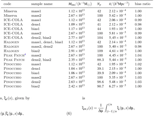
Table 1.Overview of the different samples, including the mass limits,Mlim, expressed in units of1013h−1M, the corresponding number of particles,Np, the mean number density,n¯, and the bias ratio to the corresponding Minerva parent sample,hξapp/ξMin
1/2
i. The sample names “mass”, “dens”, and “bias”, indicate if the samples were constructed by matching the mass threshold, number density, or clustering amplitude of the parent halo samples from Minerva.
code sample name Mlim/ h−1M
Np n¯/ h3Mpc−3
bias ratio Minerva mass1 1.12×10¹³ 42 2.12×10⁻⁴ 1.00 Minerva mass2 2.67×10¹³ 100 5.42×10⁻⁴ 1.00
ICE-COLA mass1 1.12×10¹³ 42 2.06×10⁻⁴ 0.99
ICE-COLA dens1 1.09×10¹³ 41 2.12×10⁻⁴ 0.98
ICE-COLA bias1 1.17×10¹³ 44 1.93×10⁻⁴ 1.00
ICE-COLA mass2 2.67×10¹³ 100 5.81×10⁻⁵ 0.99
ICE-COLA dens2, bias2 2.77×10¹³ 104 5,45×10⁻⁵ 1.00
Halogen mass1, dens1, bias1 1.12×10¹³ 42 2.14×10⁻⁴ 1.00
Halogen mass2, dens2 2.67×10¹³ 100 5,40×10⁻⁵ 0.98
Halogen bias2 2.91×10¹³ 109 4,61×10⁻⁵ 1.00
Peak Patch4 mass2 2.67×10¹³ 100 4,45×10⁻⁵ 1.04
Peak Patch dens2, bias2 2.35×10¹³ 88.3 5,44×10⁻⁵ 1.00
Pinocchio mass1 1.12×10¹³ 42 1.95×10⁻⁴ 1.02
Pinocchio dens1 1.04×10¹³ 39.1 2.15×10⁻⁴ 1.00
Pinocchio bias1 1.06×10¹³ 39.9 2.09×10⁻⁴ 1.00
Pinocchio mass2 2.67×10¹³ 100 5.35×10⁻⁵ 1.03
Pinocchio dens2 2.63×10¹³ 98.6 5.48×10⁻⁵ 1.03
Pinocchio bias2 2.42×10¹³ 90.7 6.27×10⁻⁵ 1.00 Legendre multipoles,ξ`(s), given by
ξ`(s) =
2`+1 2
Z1
−1
L`(µ)ξ(µ,s)dµ, (6)
where L`(µ) denotes the Legendre polynomial of order `.
Typically, only multipoles with`≤4are considered. An al-ternative tool is the clustering wedges statistic (Kazin et al. 2012), which corresponds to the average of the full two-dimensional correlation function over wide bins in µ, that
is
ξw,i(s) = 1
∆µ
Zi/n
(i−1)/nξ
(µ,s)dµ, (7)
whereξw,i denotes each individual clustering wedge, andn represents the total number of wedges. We follow the recent analysis ofS´anchez et al.(2017) and divide theµrange from
0 to 1 into three equal-width intervals,i=1,2,3.
boundary conditions, the fullξ(s,µ)can be computed using
the natural estimator, namely
ξ(s,µ) =DD(s,µ)
RR(s,µ)−1, (8)
where DD(s,µ) are the normalized data pair counts and RR(s,µ) the normalized random pair counts, which can be
computed as the ratio of the volume of a shelldVand the to-tal box volumeVs,RR=dV/Vs. The obtainedξ(s,µ)can be
used to estimate Legendre multipoles and clustering wedges using equations (6) and (7), respectively. We consider scales in the range20h−1Mpc≤s≤160h−1Mpcfor all our measure-ments and implement a binning scheme withds=10h−1Mpc for the following analysis. For illustration purposes we also use a binning ofds=5h−1Mpcfor the figures showing cor-relation function measurements. Considering Legendre mul-tipoles with` <4and threeµ wedges, the dimension of the total data vector,ξξξ, containing all the measured statistics
is the same in both cases (Nb=42andNb=84for the cases ofds=10h−1Mpcandds=5h−1Mpc, respectively).
3.3 Covariance matrix estimation
It is commonly assumed that the likelihood function of the measured two-point correlation function is Gaussian in form,
−2 lnL(ξξξ|θθθ) = (ξξξ−ξξξtheo(θθθ))tΨΨΨ(ξξξ−ξξξtheo(θθθ)) (9) whereξξξtheorepresents the theoretical model of the measured statistics, which here correspond to the Legendre multipoles or clustering wedges, for the parametersθθθ, andΨΨΨis the
pre-cision matrix, given by the inverse of the covariance matrix,
Ψ ΨΨ=C−1.
The covariance matrix, C is usually estimated from a large set ofNsmock catalogues as
Ci j= 1 Ns−1
Ns
∑
k=1
(ξik−ξ¯i)(ξkj−ξ¯j), (10)
where ξ¯i=N1s∑kξik is the mean value of the measurements at the i-th bin and ξik is the corresponding measurement from thek-th mock. This estimator has the advantage over other techniques such as Jackknife estimates from the data or theoretical modelling, that it tends to be less affected by biases than estimates from the data and does not require any assumptions regarding the properties of the true covariance matrix. However, the noise inCdue to the finite number of realizations leads to an additional uncertainty, which must be propagated into the final parameter constraints (Taylor et al. 2013;Dodelson & Schneider 2013;Percival et al. 2014; Sellentin & Heavens 2016). Depending on the analysis con-figuration, the control of this additional error might require a large number of realizations, withNsin the range of a few thousands. For the new generation of large-volume surveys such asEuclid, the construction of a large number of mock catalogues might be extremely demanding and will need to rely, at least partially, on approximate N-body methods. The goal of our analysis is to test the impact on the obtained pa-rameter constraints of using estimates ofCbased on different approximate methods.
We use equation (10) to compute the covariance matri-ces associated with the measurements of the multipoles and
clustering wedges of the halo samples defined in Section3.1. In order to reduce the noise in these measurements due to the limited number of realizations, we obtain three sepa-rate estimates ofCfrom each sample by treating each axis of the simulation boxes as the line-of-sight direction when computingξ(s,µ). Our final estimates correspond to the
av-erage of the covariance matrices measured on the different lines of sight. The Gaussian theoretical covariance matrices were computed for the specific number density and cluster-ing of the halo samples from Minerva. We used as input the model of the two-dimensional power spectrum described in Section3.4, whose parameters were fitted to reproduce the clustering of parent halo samples.
3.4 Testing the impact of approximate methods for covariance matrix estimates
The cosmological information recovered from full-shape fits to anisotropic clustering measurements is often expressed in terms of the BAO shift parameters
α⊥=DA
(z)r0d D0A(z)rd
, (11)
αk=H 0(z)r0
d H(z)rd
, (12)
whereH(z)is the Hubble parameter at redshift z,DA(z) is the corresponding angular diameter distance,rdis the sound horizon at the drag redshift, and the primes denote quan-tities in the fiducial cosmology; and the RSD parameter combination fσ8(z), where f(z) represents the logarithmic growth rate of density fluctuations andσ8(z) is the linear rms mass fluctuation in spheres of radius8h−1Mpc.
The constraints on these parameters are sensitive to de-tails in the definition of the likelihood function, such as the way in which the covariance matrix of the measurements is estimated. In order to asses the impact of using approxi-mate methods to estiapproxi-mateC, we perform full-shape fits of anisotropic clustering measurements in configuration space to obtain constraints on α⊥, αk, and fσ8(z) assuming the Gaussian likelihood function of equation (9). We compare the constraints obtained when C is estimated from a set of full N-body simulations with the results inferred from the same set of measurements when the covariance matrix is computed using the approximate methods described in Sec.2.
Our fits are based on the same model of the full two-dimensional correlation functionξ(µ,s)as in the analyses of the final BOSS galaxy samples (S´anchez et al. 2017;Grieb et al. 2017;Salazar-Albornoz et al. 2017), and the eBOSS DR12 catalogue (Hou et al. 2018). This model includes the effects of the non-linear evolution of density fluctuations based on gRPT (Crocce et al . in prep.) bias (Chan & Scoc-cimarro 2012), and redshift-space distortions (Scoccimarro et al. in prep.). The only difference between the model im-plemented in these studies and the one used here is that, since we analyse halo samples instead of galaxies, we do not include the so-called fingers-of-God factor,W∞(k,µ)(see
20 40 60 80 100 120 140 160
s/[h
1
Mpc]
0
50
100
150
s
2
Fit
N body,
0N body,
2N body,
420 40 60 80 100 120 140 160
s/[h
1
Mpc]
50
0
50
100
150
200
250
s
2
Fit
N body,
0N body,
2N body,
420 40 60 80 100 120 140 160
s/[h
1
Mpc]
50
0
50
100
150
200
w
s
2
Fit
N body,
w1N body,
w2N body,
w320 40 60 80 100 120 140 160
s/[h
1
Mpc]
100
0
100
200
300
w
s
2
Fit
N body,
w1N body,
w2N body,
w3Figure 2.Comparison of the mean correlation function multipoles (upper panels) and clustering wedges (lower panels) of the mass1 and mass2 samples (left and right panels, respectively) drawn from our Minerva N-body simulations, and the model described in Section3.4. The points with error bars show to the simulation results and the dashed lines correspond to the fit to these measurements. The error bars on the measurements correspond to the dispersion inferred from the 300 Minerva realizations. In all cases, the model predictions show good agreement with the N-body measurements.
b2, and the non-local bias γ3−. We explore this parameter
space by means of the Monte Carlo Markov Chain (MCMC) technique. This analysis set-up matches that of the covari-ance matrix comparison in Fourier space of our companion paperBlot et al.(2018).
In order to ensure that the model used for the fits has no impact on the covariance matrix comparison, we do not fit the measurements of the Legendre multipoles and wedges obtained from the N-body simulations. Instead, we use our baseline model to construct synthetic clustering measure-ments, which we then use for our fits. For this, we first fit the mean Legendre multipoles measured from the parent Mineva halo samples using our model and the N-body covari-ance matrices. We fix all cosmological parameters to their true values and only vary the bias parameters b1,b2, and γ3−. We then use the mean values of the parameters inferred
from the fits, together with the true values of the cosmologi-cal parameters, to generate multipoles and clustering wedges of the correlation function using our baseline model. Fig.2 shows the mean multipoles and clustering wedges measured from the Minerva halo sample for both mass cuts and the re-sulting fits. In all cases, our model gives a good description of the simulation results. The parameter values recovered from these fits were also used to compute the input power spectra when computing the Gaussian predictions ofC. As
these synthetic data are perfectly described by our base-line model by construction, their analysis should recover the true values of the BAO parametersαk=α⊥=1.0, and the
growth-rate parameter fσ8=0.4402. The comparison of the parameter values and their uncertainties recovered using dif-ferent covariance matrices allows us to test the ability of the approximate methods described in Section 2 to reproduce the results obtained when C is inferred from full N-body simulations.
4 RESULTS
In this section, we present a detailed comparison of the co-variance matrix measurements in configuration space ob-tained from the approximate methods described in Section2 and their performance at recovering the correct parameter estimates.
4.1 Two-point correlation function measurements
−50 −25 0 25 50 75 100 125
ξ
0·
s
2
“
dens1
”
ICE−COLA
PINOCCHIO
N−body
−0.005
∆
ξ
0−−80100 −60 −40 −20 0
ξ
2·
s
2
−0.05 0.00 0.05
∆
ξ
2−40 −20 0 20 40
ξ
4·
s
2
20 40 60 80 100 120 140 160
s
/
[
h
−1Mpc
]
−0.025 0.025
∆
ξ
4multipoles
HALOGEN PATCHY
log−normal,
N−body
40 60 80 100 120 140 160
s
/
[
h
−1Mpc
]
−50 0 50 100 150 200 250
ξ
w1·
s
2
“
bias2
”
ICE−COLA
PINOCCHIO Peak Patch
N−body
−0.050 0.000
∆
ξ
w1−50 0 50 100 150 200
ξ
w2·
s
2
−0.05 0.05
∆
ξ
w2−100 −50 0 50 100
ξ
w3·
s
2
20 40 60 80 100 120 140 160
s
/
[
h
−1Mpc
]
−0.05 0.05
∆
ξ
w3wedges
HALOGEN PATCHY
log−normal
N−body
40 60 80 100 120 140 160
s
/
[
h
−1Mpc
]
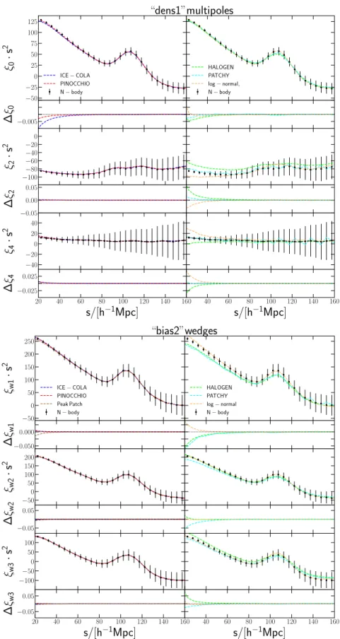
Figure 3.Upper panel: measurements of the mean multipoles for the density matched samples for the first mass cut (dens1 samples). The first, third and fifth row show the monople, quadrupole and hexadecapole, respectively.Lower panel: measurements of the mean clustering wedges for the bias matched samples for the second mass cut (bias2 samples). The first, third and fifth row show the transverse, intermediate and parallel wedge, respectively. Comparison of the measurements drawn from the results of the predictive methods ICE-COLA and Pinocchio (left panels) and the calibrated methodsHalogen and Patchy and the log-normal model (right panels) to
wedges for each sample and in each realization as described in Section3.2.
As an illustration of the agreement between the cluster-ing measurements obtained from the approximate methods and the Minerva simulations we focus here on two cases: i) the multipoles of the density-matched samples for the first mass cut (dens1 samples), and ii) the clustering wedges of the bias-matched samples for the second mass cut (bias2 samples). As described in Section3.1, forPatchyand the log-normal realizations, the density- and bias-matched sam-ples are identical to the mass-matched samsam-ples by construc-tion.
The upper panel of Fig. 3 shows the mean multipole measurements from all realizations for the dens1 samples ob-tained from the predictive methodsICE-COLAand Pinoc-chio (left panels) and the calibrated methods Halogen, Patchy, and the log-normal recipe (right panels). The pre-dictive methods are in excellent agreement with the mea-surements from the Minerva parent sample, showing only differences of less than 3% for the ICE-COLA monopole measurements on scales <40h−1Mpc. The monopole mea-surements obtained from the calibrated methods and the log-normal model are also in good agreement with the re-sults from Minerva. However, the quadrupole and hexade-capole measurements obtained fromHalogenand the log-normal samples exhibit deviations of more than 20% on scales<60h−1Mpc.
The lower panel of Fig.3shows the mean wedges mea-surements from all realizations for the bias2 samples ob-tained from the predictive methods ICE-COLA, Pinoc-chioandPeak Patch(left panels), and for the correspond-ing samples obtained from calibrated methods Halogen, Patchy, and the log-normal recipe (right panels). Here we find that the measurements obtained from the predictive methods and the log-normal model agree well within the error bars with the corresponding Minerva measurements. We notice that the strongest deviations are present in the measurements of the transverse and parallel wedge from the Halogen samples, of up to 6% and 20% respectively on scales <60h−1Mpc. The measurements recovered from
Patchy show deviations ranging between 5% to 10% on
small scales.
4.2 Covariance matrix measurements
In this section we focus on the comparison of the covariance matrix estimates obtained from the different approximate methods, which we computed as described in Section3.3.
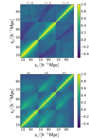
The structure of the off-diagonal elements ofC of Leg-endre multipoles and clustering wedges measurements can be more clearly seen in the correlation matrix, defined as
Ri j= Ci j
p CiiCj j
. (13)
Fig.4 shows the correlation matrices of the multipoles in-ferred from the mass1 halo samples from Minerva (upper panel) and the wedges of the mass2 samples (lower panel).
The estimates of R obtained from the approximate methods are indistinguishable by eye from the ones inferred from the Minerva parent samples and therefore not shown here. Instead, we compare the variances and cuts through the correlation function matrices derived from the different
10 90 10 90 10 90
s
i
/
[
h
−1
Mpc
]
10
90
10
90
10
90
s
j
/
[
h
−
1
M
pc
]
l
= 0
l
= 2
l= 4
0.4
0.2
0.0
0.2
0.4
0.6
0.8
1.0
10 90 10 90 10 90
s
i
/
[
h
−1
Mpc
]
10
90
10
90
10
90
s
j
/
[
h
−
1
M
pc
]
w
1
w2
w3
0.4
0.2
0.0
0.2
0.4
0.6
0.8
1.0
Figure 4.The full correlation matrix inferred from the multipoles of the N-body parent sample for the low-mass cut (mass1, upper panel) and from the clustering wedges of the mass2 N-body parent sample (lower panel).
samples. Fig.5shows the ratios of the variances drawn from the approximate methods with respect to those of the corre-sponding Minerva parent catalogues. We focus here on the same example cases as in Section4.1: the multipoles mea-sured from the dens1 samples, and the clustering wedges measured from the bias2 samples. We notice that in both cases the predictive methods perform better than the cali-brated schemes and the PDF-based recipes. On average, the variance from Minerva is recovered within 10%, with a max-imum difference of 20% for the variance of the monopole inferred from thePinocchiodens1 sample at scales around 80h−1Mpc. The variances recovered from the other methods show larger deviations, in some cases up to 40%.
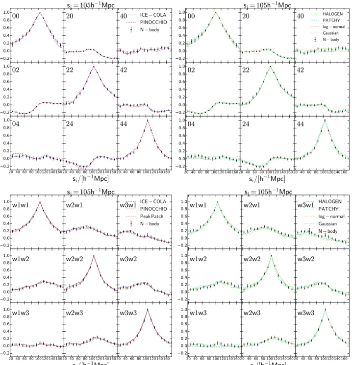
Fig.6shows cuts through the correlation matrix atsj= 105h−1Mpcfor the same two example cases. The error bars for the measurements of the corresponding Minerva parent samples are obtained from a jackknife estimate using the 300 Minerva mocks,
(∆Mi j)2= NS−1
NS
∑
S(M(i js)−Mi j)2, (14)
R (for Fig. 6 we useR). M(s) is the covariance or correla-tion matrix which is obtained when leaving out the s−th realization,
Mi j(s)= 1 NS−1r
∑
6=s(ξi(r)−ξ¯i)(ξ(jr)−ξ¯j). (15)
For the comparison of the cuts through the correlation matrices, all methods agree well the corresponding N-body measurements with only very small differences. In order to quantify the discrepancies between the covariance and cor-relation matrices drawn from the approximate methods to the corresponding N-body measurements, we use anχ2
ap-proach. Concretely, we computeχ2 as
χ2=
∑
i
∑
j≥i(Ci j,approx−Ci j,Minerva)2
∆C2i j,Minerva , (16)
and
χ2=
∑
i∑
j>i(Ri j,approx−Ri j,Minerva)2
∆R2i j,Minerva , (17)
where the indicesiand jrun over the bins corresponding to the range of interest of20−160h−1Mpc and∆CMinerva and
∆RMinerva are the estimated errors from equation (14). If the approximate methods perfectly reproduce the expected covariances from the N-body simulations, the χ2 obtained
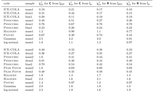
from the approximate methods should beχ2≈0for the pre-dictive and calibrated methods. This is due to the fact that the simulation boxes of the predictive and calibrated meth-ods match the initial conditions of Minerva and therefore the properties of the noise in the estimates ofCshould be very similar. For the covariance and correlation matrices obtained from the PDF-based predictions, we expectχ2≈N(N−1)/2 where N is the number of bins of the covariance or corre-lation matrix, since these predictions do not correspond to the same initial conditions. In table 2we list the obtained relativeχ2-values,
χrel2 =
χ2
N(N−1)/2, (18)
where N =42, for all considered samples and clustering statistics. We notice that the χ2-values are in most cases
smaller for the predictive than the calibrated methods. Fur-thermore, theχ2-values from the wedges measurements are
overall smaller than the corresponding ones from the mul-tipole measurements. Also, in most cases the χ2-values
ob-tained from the covariance matrices are slightly larger than the corresponding ones from the correlation matrices, in-dicating discrepancies in the variances obtained from the approximated methods.
4.3 Performance of the covariance matrices
For the final validation of the covariance matrices inferred from the different approximate methods, we analyse their performance on cosmological parameter constraints. We per-form fits to the synthetic clustering measurements described in Section3.4, using the estimates ofC obtained from the different halo samples and approximate methods. We focus on the constraints on the BAO shift parametersαk,α⊥, and the growth rate fσ8.
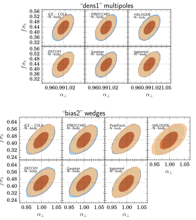
Fig. 7 shows the two-dimensional marginalised con-straints in theα⊥-fσ8 plane for the analysis of our two ex-amples cases, the Legendre multipoles measured from the dens1 samples (upper panels), and the clustering wedges re-covered from the bias2 samples (lower panel).
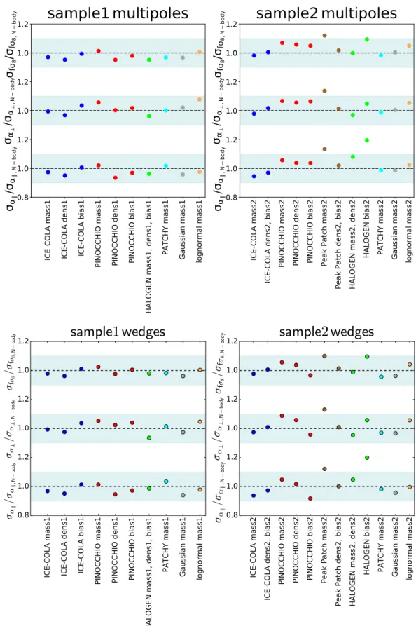
In general, the allowed regions for these parameters ob-tained using the estimates ofCinferred from the different ap-proximate methods (shown by the solid lines) agree well with those obtained using the covariance matrices from Minerva (indicated by the dotted lines in all panels). However, most cases exhibit small deviations, either slightly under- or over-estimating the statistical uncertainties. We find that, for all samples and clustering statistics, the mean parameter values inferred using approximate methods are in excellent agree-ment with the ones from the corresponding N-body analysis, showing differences that are much smaller than their asso-ciated statistical errors. The parameter uncertainties recov-ered using covariances from the approximate methods show differences with respect to the N-body constraints ranging between 0.3% and 8% for the low mass samples, while most of the results agree within 5% with the N-body results, and between 0.1% and 20% for the high-mass cut, while most of the results agree within 10% with the N-body results. For the comparison of the obtained parameter uncertainties it is important to point out that in our companion paperBlot et al.(2018) estimate that the statistical limit of our param-eter estimation is about 4% to 5%. Fig.8shows the ratios of the marginalised parameter errors drawn from the analy-sis with the different approximate methods with respect to the N-body results. We observe that for the samples corre-sponding to the first mass cut, all methods reproduce the N-body errors within 10% for all parameters, and in most cases within 5% corresponding to the statistical limit of our analysis. For the samples corresponding to the second mass cut also most methods reproduce the N-body errors within 10% with exception of thePeak Patchmass-matched and theHalogenbias-matched samples. This might be due to the fact that these two samples have 15-20% less halos than the corresponding N-body sample.
In order to evaluate the parameter errors, we use the volume of the allowed region in the three-dimensional pa-rameter space ofαk,α⊥and fσ8, which can be estimated as
V=qdet Cov(αk,α⊥,fσ8) (19)
−
0
.
4
−
0
.
2
0
.
0
0
.
2
0
.
4
∆
σ
2 0
/σ
2 0,N−
b
ody
“
dens1
”
ICE−COLA
PINOCCHIO
−
0
.
4
−
0
.
2
0
.
0
0
.
2
0
.
4
∆
σ
2 2
/σ
2 2,N−
b
ody
40
60
80 100 120 140
s
/
[
h
−1Mpc
]
−
0
.
4
0
.
0
0
.
4
∆
σ
2 4
/σ
2 4,N−
b
ody
multipoles
HALOGEN PATCHY
log−normal
Gaussian
40
60
80 100 120 140
s
/
[
h
−1Mpc
]
−
0
.
4
−
0
.
2
0
.
0
0
.
2
0
.
4
∆
σ
2 w1
/σ
2 w1,
N
−
b
ody
“
bias2
”
ICE−COLA
PINOCCHIO PeakPatch
−
0
.
4
−
0
.
2
0
.
0
0
.
2
0
.
4
∆
σ
2 w2
/σ
2 w2,
N
−
b
ody
40
60
80 100 120 140
s
/
[
h
−1Mpc
]
−
0
.
4
0
.
0
0
.
4
∆
σ
2 w3
/σ
2 w3,N
−
b
ody
wedges
HALOGEN PATCHY
log−normal
Gaussian
40
60
80 100 120 140
s
/
[
h
−1Mpc
]
0.2 0.0 0.2 0.4 0.6 0.8 1.0
00
20
s
j= 105
h
−1Mpc
40
ICE−COLAPINOCCHIO
N−body
0.2 0.0 0.2 0.4 0.6 0.8 1.0
02
22
42
20 40 60 80 100120140160 0.2
0.0 0.2 0.4 0.6 0.8 1.0
04
20 40 60 80 100120140160
s
i/
[
h
−1Mpc
]
24
20 40 60 80 100120140160
44
0.2 0.0 0.2 0.4 0.6 0.8
1.0
w
1
w
1
w
2
w
1
s
j= 105
h
−1Mpc
w
3
w
1
ICEPINOCCHIO−COLAPeak Patch
N−body
0.2 0.0 0.2 0.4 0.6 0.8
1.0
w
1
w
2
w
2
w
2
w
3
w
2
20 40 60 80 100120140160 0.2
0.0 0.2 0.4 0.6 0.8
1.0
w
1
w
3
20 40 60 80 100120140160
s
i/
[
h
−1Mpc
]
w
2
w
3
20 40 60 80 100120140160
w
3
w
3
0.2 0.0 0.2 0.4 0.6 0.8 1.0
00
20
s
j= 105
h
−1Mpc
40
HALOGENPATCHY log−normal Gaussian N−body
0.2 0.0 0.2 0.4 0.6 0.8 1.0
02
22
42
20 40 60 80 100120140160 0.2
0.0 0.2 0.4 0.6 0.8
1.0
04
20 40 60 80 100120140160
s
i/
[
h
−1Mpc
]
24
20 40 60 80 100120140160
44
0.2 0.0 0.2 0.4 0.6 0.8
1.0
w
1
w
1
w
2
w
1
s
j= 105
h
−1Mpc
w
3
w
1
HALOGENPATCHYlog−normal
Gaussian
N−body
0.2 0.0 0.2 0.4 0.6 0.8
1.0
w
1
w
2
w
2
w
2
w
3
w
2
20 40 60 80 100120140160 0.2
0.0 0.2 0.4 0.6 0.8
1.0
w
1
w
3
20 40 60 80 100120140160
s
i/
[
h
−1Mpc
]
w
2
w
3
20 40 60 80 100120140160
w
3
w
3
Figure 6.Cuts atsj=105h−1Mpc through the correlation matrices for the two example cases drawn from the results of the approximate methods and the corresponding N-body parent sample. Upper, left panel: Correlation matrices measured from the multipoles of the correlation function drawn from dens1 samples from the predictive methodsICE-COLAandPinocchio.Upper, right panel: Correlation matrices measured from the multipoles of the correlation function drawn from dens1 samples from the calibrated methodsHalogenand
Patchyand the Gaussian and log-normal recipes.Lower, left panel: Correlation matrices measured from the clustering wedges of the
correlation function drawn from the bias2 samples from the predictive methodsICE-COLA,PinocchioandPeak Patch.Lower, right
panel: Correlation matrices measured from the clustering wedges of the correlation function drawn from bias2 samples from the calibrated
methodsHalogenandPatchyand the Gaussian and log-normal recipes. The error bars are obtained from a jackknife estimate using the 300 Minerva realizations.
the samples. The results from the majority of the samples agree within 10% with the N-body results, the rest shows dif-ferences of 10%–15%, and for the Peak Patchmass2 and Halogenbias2 samples differences of up to 40%. For both mass cuts, we find significant differences in the performances