Comparison of Einstein-Boltzmann solvers for testing general relativity
E. Bellini,1 A. Barreira,2 N. Frusciante,3 B. Hu,4 S. Peirone,5M. Raveri,6 M. Zumalacárregui,7,8 A. Avilez-Lopez,9 M. Ballardini,10,11,12,13 R. A. Battye,14B. Bolliet,15E. Calabrese,1,16Y. Dirian,17P. G. Ferreira,1 F. Finelli,12,13 Z. Huang,18M. M. Ivanov,19,20J. Lesgourgues,21B. Li,22N. A. Lima,23F. Pace,14D. Paoletti,12,13 I. Sawicki,24
A. Silvestri,5 C. Skordis,24,25C. Umilt`a,26,27,28 and F. Vernizzi29 1
University of Oxford, Denys Wilkinson Building, Keble Road, Oxford OX1 3RH, United Kingdom 2Max-Planck-Institut für Astrophysik, Karl-Schwarzschild-Str. 1, 85741 Garching, Germany 3
Instituto de Astrofisica e Ciencias do Espaco, Faculdade de Ciencias da Universidade de Lisboa, Edificio C8, Campo Grande, P-1749016 Lisboa, Portugal
4
Department of Astronomy, Beijing Normal University, Beijing 100875, China 5Institute Lorentz, Leiden University, PO Box 9506, Leiden 2300 RA, The Netherlands 6
Kavli Institute for Cosmological Physics, Enrico Fermi Institute, The University of Chicago, Chicago, Illinois 60637, USA
7
Nordita, KTH Royal Institute of Technology and Stockholm University, Roslagstullsbacken 23, SE-106 91 Stockholm, Sweden
8
Berkeley Center for Cosmological Physics, LBL and University of California at Berkeley, California 94720, USA
9
Departamento de Física, Centro de Investigación y de Estudios Avanzados del IPN, AP 14-740, Ciudad de M´exico 07000, Mexico
10
Department of Physics and Astronomy, University of the Western Cape, Cape Town 7535, South Africa 11DIFA, Dipartimento di Fisica e Astronomia, Alma Mater Studiorum Universit `a di Bologna,
Viale Berti Pichat, 6/2, I-40127 Bologna, Italy 12INAF/IASF Bologna, via Gobetti 101, I-40129 Bologna, Italy 13
INFN, Sezione di Bologna, Via Berti Pichat 6/2, I-40127 Bologna, Italy
14Jodrell Bank Centre for Astrophysics, School of Physics and Astronomy, The University of Manchester,
Manchester M13 9PL, United Kingdom
15Laboratoire de Physique Subatomique et de Cosmologie, Universit´e Grenoble-Alpes,
CNRS/IN2P3 53, avenue des Martyrs, 38026 Grenoble cedex, France 16School of Physics and Astronomy, Cardiff University,
The Parade, Cardiff CF24 3AA, United Kingdom
17D´epartement de Physique Th´eorique and Center for Astroparticle Physics, Universit´e de Gen`eve,
24 quai Ansermet, CH-1211 Gen`eve 4, Switzerland
18School of Physics and Astronomy, Sun Yat-sen University, 2 Daxue Road, Zhuhai 519082, China 19
Institute of Physics, LPPC, École Polytechnique F´ed´erale de Lausanne, CH-1015 Lausanne, Switzerland
20
Institute for Nuclear Research of the Russian Academy of Sciences, 60th October Anniversary Prospect, 7a, 117312 Moscow, Russia 21
Institute for Theoretical Particle Physics and Cosmology (TTK), RWTH Aachen University, D-52056 Aachen, Germany
22
Institute for Computational Cosmology, Department of Physics, Durham University, Durham DH1 3LE, United Kingdom
23
Institut für Theoretische Physik, Universität Heidelberg, Philosophenweg 16, D-69120 Heidelberg, Germany 24
CEICO, Fyzikální ustáv Akademie vědČR, Na Slovance 1999/2, 182 21 Prague, Czech Republic 25Department of Physics, University of Cyprus, 1, Panepistimiou Street, 2109 Aglantzia, Cyprus 26
Institut d’Astrophysique de Paris, CNRS (UMR7095), 98 bis Boulevard Arago, F-75014 Paris, France 27UPMC Univ Paris 06, UMR7095, 98 bis Boulevard Arago, F-75014 Paris, France
28
Sorbonne Universit´es, Institut Lagrange de Paris (ILP), 98 bis Boulevard Arago, 75014 Paris, France 29Institut de Physique Th´eorique, Universit´e Paris Saclay,
CEA, CNRS, 91191 Gif-sur-Yvette, France
(Received 6 October 2017; published 22 January 2018)
models Hoˇrava-Lifschitz gravity, and two codes that model nonlocal models of gravity. Comparing predictions of the angular power spectrum of the cosmic microwave background and the power spectrum of dark matter for a suite of different models, we find agreement at the subpercent level. This means that this suite of Einstein-Boltzmann solvers is now sufficiently accurate for precision constraints on cosmological and gravitational parameters.
DOI:10.1103/PhysRevD.97.023520
I. INTRODUCTION
Parameter estimation has become an essential part of modern cosmology, e.g.,[1]. By this we mean the ability to constrain various properties of cosmological models using observational data such as the anisotropies of the cosmic microwave background (CMB), the large scale structure of the galaxy distribution (LSS), the expansion and acceler-ation rate of the Universe, and other such quantities. A crucial aspect of this endeavor is to be able to accurately calculate a range of observables from the cosmological models. This is done with Einstein-Boltzmann (EB) solv-ers, i.e., codes that solve the linearized Einstein and Boltzmann equations on an expanding background [2].
The history of EB solvers is tied to the success of modern theoretical cosmology. Beginning with the seminal work of Peebles and Yu [3], Wilson and Silk [4], Bond and Efstathiou [5], and Bertschinger and Ma [6] these first attempts involved solving coupled set of many thousands of ordinary differential equations in a time consuming, com-puter intensive manner. A step change occurred with the introduction of the line of sight method and theCMBFAST code[7]by Seljak and Zaldarriaga, which sped calculations up by orders of magnitude. Crucial in establishing the reliability ofCMBFASTwas a cross comparison[8]between a handful of EB solvers (includingCMBFAST) that showed that it was possible to get agreement to within 0.1%. Fast EB solvers have become the norm: CAMB[9], DASh[10], CMBEASY [11], and CLASS [12,13]all use the line of sight approach and have been extensively used for cos-mological parameters estimation. Of these, CAMB and CLASS are kept up to date and are, by far, the most widely used as part of the modern armoury of cosmological analysis tools.
While CAMB and CLASS were developed to accurately model the standard cosmology—general relativity with a cosmological constant—there has been surge in interest in testing extensions that involve modifications to gravity
[14]. Indeed, it has been argued that it should be possible to test general relativity (GR) and constrain the associated gravitational parameters to the same level of precision as with other cosmological parameters. More ambitiously, one hopes that it should be possible to test GR on cosmological scales with the same level of precision as is done on astrophysical scales [15]. Two types of codes have been developed for the purpose of achieving this goal: general purpose codes which are either not tied to any specific
theory (such asMGCAMB[16]andISITGR[17]) or model a broad class of (scalar-tensor) theories (such as EFTCAMB
[18]andhi_class[19]) and specific codes which model targeted theories such as Jordan-Bran-Dicke gravity[20], Einstein-Aether gravity[21],fðRÞ[22], covariant galileons
[23], and others.
The stakes have changed in terms of theoretical precision. Up and coming surveys such as Euclid,1 LSST,2WFIRST,3 SKA,4and Stage 4 CMB5experiments all require subpercent agreement in theoretical accuracy (cosmic variance is inversely proportional to the angular wave number probed,l, and we expect to at most, reach
l∼few ×103). While there have been attempts at check-ing and calibratcheck-ing existcheck-ing non-GR N-body codes [24], until now the same effort has not been done for non-GR EB solvers with this accuracy in mind. In this paper we attempt to repeat what was done in[8,25]with a handful of codes. We will focus on scalar modes, neglecting for simplicity primordial tensor modes and B-modes of the CMB. In particular, we will show that two general purpose codes— EFTCAMBandhi_class—agree with each other to a high level of accuracy. The same level of accuracy is reached with the third general purpose code—COOP; however, the latter code needs further calibration to maintain agreement at sub-Mpc scales. We also show that they agree with a number of other EB solvers for a suite of models such Jordan-Brans-Dicke (JBD), covariant Galileons,fðRÞ, and Hoˇrava-Lifshitz (khronometric) gravity. And we will show that for some models not encompassed by these general purpose codes, i.e., nonlocal theories of gravity, there is good agreement between existing EB solvers targeting them. This gives us confidence that these codes can be used for precision constraints on general relativity using observ-ables of a linearly perturbed universe.
We structure our paper as follows. In Sec.IIwe lay out the formalism used in constructing the different codes and we summarize the theories used in our comparison. In Sec.III
we describe the codes themselves, highlighting their key features and the techniques they involve. In Sec. IV we compare the codes in different settings. We begin by
comparing the codes for specific models and then choose different families of parametrizations for the free functions in the general purpose codes. In Sec.Vwe discuss what we have learnt and what steps to take next in attempts at improving analysis tools for future cosmological surveys.
II. FORMALISM AND THEORIES
To study cosmological perturbations on large scales, one must expand all relevant cosmological fields to linear order around a homogeneous and isotropic background. By cosmological fields we mean the space time metric, gμν, the various components of the energy density,ρi(where i can stand for baryons, dark matter, and any other fluid one might consider), the pressure, Pi, and momentum, θi, as well as the phase space densities of the relativistic compo-nents,fj(wherejnow stands for photons and neutrinos) as well as any other exotic degree of freedom (d.o.f.), (such as, for example, a scalar field, ϕ, in the case of quintessence theories). One then replaces these linearized fields in the cosmological evolution equations; specifically in the Einstein field equations, the conservation of energy momentum tensor and the Boltzmann equations. One can then evolve the background equations and the linear-ized evolution equations to figure out how a set of initial perturbations will evolve over time.
The end goal is to be able to calculate a set of spectra. First, the power spectrum of matter fluctuations at con-formal time τ defined by
hδ
Mðτ;k0ÞδMðτ;kÞi≡ð2πÞ3Pðk;τÞδ3ðk−k0Þ; ð1Þ where we have expanded the energy density of matter,ρM around its mean value,ρ¯M,δM¼ ðρM−ρ¯MÞ=ρ¯M, and taken its Fourier transform. Second, the angular power spectrum of CMB anisotropies
hal0m0almi ¼CTTl δll0δmm0; ð2Þ
where we have expanded the anisotropies, δT=TðnˆÞ in spherical harmonics such that
δT T ðnˆÞ ¼
X
lm
almYlmðnˆÞ: ð3Þ
More generally one should also be able to calculate the angular power spectrum of polarization in the CMB, spe-cifically of the“E”mode,CEE
l , the“B”mode,CBBl and the cross-spectra between the E mode and the temperature anisotropies, CTEl , as well as the angular power spectrum of the CMB lensing potential,Cϕϕl . As a by-product, one can also calculate“background”quantities such as the history of the Hubble rate,HðτÞ, the angular-distance as a function of redshift,DAðzÞand other associated quantities such as the luminosity distance,DLðzÞ.
To study deviations from general relativity, one needs to consider two main extensions. First one needs to include
extra, gravitational d.o.f. In this paper we will restrict ourselves to scalar-tensor theories, as these have been the most thoroughly studied, and furthermore we will consider only one extra d.o.f. This scalar field, and its perturbation, will have an additional evolution equation which is coupled to gravity. Second, there will be modifications to the Einstein field equations and their linearized form will be modified accordingly. How the field equations are modified and how the scalar field evolves depends on the class of theories one is considering. In what follows, we will describe what these modifications mean for different classes of scalar-tensor theories and also theories that evolve restricted scalar d.o.f. (such as Hoˇrava-Lifshitz and non-local theories of gravity).
A. The effective field theory of dark energy
A general approach to study scalar-tensor theories is the so-called effective field theory of dark energy (EFT)[26– 37]. Using this approach, it is possible to construct the most general action describing perturbations of single field dark energy (DE) and modified gravity models (MG). This can be done by considering all possible operators that satisfy spatial-diffeomorphism invariance, constructed from the metric in unitary gauge where the time is chosen to coincide with uniform field hypersurfaces. The operators can be ordered in number of perturbations and derivatives. Up to quadratic order in the perturbations, the action is given by
S¼ Z
d4xpffiffiffiffiffiffi−g
M2Pl
2 ½1þΩðτÞRþΛðτÞ−a2cðτÞδg00
þM42ðτÞ
2 ða2δg00Þ2− ¯ M31ðτÞ
2 a2δg00δKμμ− ¯ M22ðτÞ
2 ðδKμμÞ2 −M¯23ðτÞ
2 δKμνδKνμþ
a2Mˆ2ðτÞ
2 δg00δRð3Þ þm22ðτÞðgμνþnμnνÞ∂μða2g00Þ∂νða2g00Þ þ
þSm½χi; gμν; ð4Þ
whereRis the 4D Ricci scalar andnμdenotes the normal to the spatial hypersurfaces; Kμν¼ ðδρμþnρnμÞ∇ρnν is the extrinsic curvature, K its trace, and Rð3Þ is the 3D Ricci scalar, all defined with respect to the spatial hypersurfaces. Moreover, we have tagged with aδall perturbations around the cosmological background. Sm is the matter action describing the usual components of the Universe, which we assume to be minimally and universally coupled to gravity. The ellipsis stand for higher order terms that will not be considered here. The explicit evolution of the perturbation of the scalar field can be obtained by applying the Stückelberg technique to Eq.(4)which means restoring the time diffeomorphism invariance by an infinitesimal time coordinate transformation, i.e.,t→tþπðxμÞ, where
π is the explicit scalar d.o.f.
background energy density and pressure, using the back-ground evolution equations obtained from this action
[26–29]. Then, the general family of scalar-tensor theories is spanned by eight functions of time, i.e., ΩðτÞ, M42ðτÞ, M2iðτÞ (withi¼1;…;3),Mˆ2ðτÞ,m22ðτÞplus one function describing the background expansion rate asH≡da=ðadtÞ.6 Their time dependence is completely free unless they are constrained to represent some particular theory. Indeed, besides their model independent characterization, a general recipe exists to map specific models in the EFT language[26– 29,32,37,38]. In other words, by making specific choices for these EFT functions it is possible to single out a particular class of scalar-tensor theory and its cosmological evolution for a specific set of initial conditions. The number of EFT functions that are involved in the mapping increases propor-tionally to the complexity of the theory. In particular, linear perturbations in nonminimally coupled theories such as Jordan-Brans-Dicke are described in terms of two indepen-dent functions of time, ΩðτÞ and HðτÞ, i.e., by setting M42¼0,M¯2i ¼0(i¼1;…;3) andm22¼0. Increasing the complexity of the theory, perturbations in Horndeski theories
[39,40] are described by setting fM¯22¼−M¯23¼2Mˆ2; m22¼0g, in which case one is left with four independent functions of time in addition to the usual dependence onHðτÞ
[28,29]. Moreover, by detuning2Mˆ2fromM¯22¼−M¯23one is considering beyond Horndeski theories [41,42]. Lorentz violating theories, such as Hoˇrava gravity[43,44], also fall in this description by assumingm22≠0.
For practical purposes, it is useful to define a set of dimensionless functions in terms of the original EFT functions as
γ1¼ M
4 2
M2PlH20; γ2¼ ¯ M31
M2PlH0; γ3¼ ¯ M22 M2Pl;
γ4¼ ¯ M23
M2Pl; γ5¼
ˆ
M2
M2Pl; γ6¼ m22
M2Pl; ð5Þ
whereH0andMPlare the Hubble parameter today and the Planck mass respectively.
In this basis, Horndeski gravity corresponds toγ4¼−γ3,
γ5¼γ23 andγ6¼0. As explained above, this reduces the number of free functions to five, i.e.,fΩ;γ1;γ2;γ3gplus a function that fixes the background expansion history. In this limit the EFT approach is equivalent to theαformalism described in the next section. Indeed, a one-to-one map to convert between the two bases is provided in AppendixA.
B. The Horndeski action
A standard approach to study general scalar-tensor theories is to write down a covariant action by considering
explicitly combinations of a metric,gμν, a scalar field,ϕ, and their derivatives. The result for the most general action leading to second-order equations of motion on any back-ground is the Horndeski action[39,45], which reads
S¼ Z
d4xpffiffiffiffiffiffi−gX 5
i¼2
Li½ϕ; gμν þSm½χi; gμν; ð6Þ
where, as always throughout this paper, we have assumed minimal and universal coupling to matter in Sm. The building blocks of the scalar field Lagrangian are
L2¼K; L3¼−G3□ϕ;
L4¼G4RþG4Xfð□ϕÞ2−∇μ∇νϕ∇μ∇νϕg;
L5¼G5Gμν∇μ∇νϕ−16G5Xfð□ϕÞ3−3∇μ∇νϕ∇μ∇νϕ□ϕ þ2∇ν∇μϕ∇α∇νϕ∇μ∇αϕg; ð7Þ
whereKandGAare functions ofϕandX≡−∇νϕ∇νϕ=2,
and the subscripts X and ϕ denote derivatives. The four functions,K andGA completely characterize this class of theories.
Horndeski theories are not the most general viable class of theories. Indeed, it is possible to construct scalar-tensor theories with higher-order equations of motion and containing a single scalar d.o.f., such as the so-called“beyond Horndeski”extension[41,42,46]. It was recently realized that higher-order scalar-tensor theories propagating a single scalar mode can be understood as degenerate theories[47–49].
It is possible to prove that the exact linear dynamics predicted by the full Horndeski action, Eq. (6), is com-pletely described by specifying five functions of time, the Hubble parameter and[50]
M2≡2ðG4−2XG4XþXG5ϕ−ϕ_HXG5XÞ;
HM2αM≡d dtM
2
;
H2M2αK≡2XðKXþ2XKXX−2G3ϕ−2XG3ϕXÞ
þ12 _ϕXHðG3XþXG3XX−3G4ϕX−2XG4ϕXXÞ þ12XH2ðG4Xþ8XG4XXþ4X2G4XXXÞ −12XH2ðG
5ϕþ5XG5ϕXþ2X2G5ϕXXÞ þ4 _ϕXH3ð3G5Xþ7XG5XXþ2X2G5XXXÞ;
HM2αB≡2 _ϕðXG3X−G4ϕ−2XG4ϕXÞ
þ8XHðG4Xþ2XG4XX−G5ϕ−XG5ϕXÞ þ2 _ϕXH2ð3G5Xþ2XG5XXÞ;
M2αT≡2X½2G4X−2G5ϕ−ðϕ̈ −ϕ_HÞG5X; ð8Þ 6Note thatHdoes not completely fix the evolution of all the
where dots are derivatives with respect to cosmic time t andH≡da=ðadtÞ.
While the Hubble parameter fixes the expansion history of the universe, theαifunctions appear only at the pertur-bation level. M2 defines an effective Planck mass, which canonically normalize the tensor modes.αKandαB(dubbed as kineticity and braiding) are respectively the standard kinetic term present in simple DE models such as quintes-sence and the kinetic term arising from a mixing between the scalar field and the metric, which is typical of MG theories as fðRÞ. Finally,αThas been namedtensor speed excess, and it is responsible for deviations on the speed of gravitational waves while on the scalar sector it generates anisotropic stress between the gravitational potentials.
It is straightforward to relate the free functionsfM;αK;
αB;αTgdefined above to the free functionsfΩ;γ1;γ2;γ3g used to describe Horndeski theories in the EFT formalism. The mapping between these sets of functions is reported in Appendix A. For an explicit expression of the functions fΩ;γ1;γ2;γ3gin terms of the originalfK; GAgin Eq.(7), we refer the reader to[37](see also[28,29]).
Regardless of the basis (αs or EFT), it is clear now that there are two possibilities. The first one is to calculate the time dependence of αi or γi and the background consis-tently to reproduce a specific sub-model of Horndeski, the second one is to specify directly their time dependence. Finally, the evolution equation for the extra scalar field and the modifications to the gravitational field equations depend solely on this set of free functions; any cosmology arising from Horndeski gravity can be modelled with an appropriate time dependence for these free functions.
C. Jordan-Brans-Dicke
The Jordan-Brans-Dicke (JBD) theory of gravity [51], a particular case of the Horndeski theory, is given by the action
S¼ Z
d4xpffiffiffiffiffiffi−gM 2 Pl 2
ϕR−ωBD
ϕ ∇μϕ∇μϕ−2V
þSm½χi; gμν; ð9Þ
whereVðϕÞis a potential term andωBDis a free parameter. GR is recovered whenωBD→∞. For our test, we will not consider a generic potential but a cosmological constant instead, Λ, as the source of dark energy.
In the EFT language, linear perturbations in JBD theories are described by two functions, i.e., the Hubble rate HðtÞ [or equivalentlycðτÞor ΛðτÞ] and
ΩðτÞ ¼ϕ−1;
γiðτÞ ¼0: ð10Þ
We can see that in this case there are no terms consisting of purely modified perturbations (i.e., any of the γi).
Alternatively the αiðτÞ functions read
αMðτÞ ¼ dlnϕ dlna;
αBðτÞ ¼−αM;
αKðτÞ ¼ωBDα2M;
αTðτÞ ¼0: ð11Þ
As with the EFT basis, one has to consider the Hubble parameter HðτÞ as an additional building function. However, HðτÞ can be written entirely as a function of theαs, meaning that the five functions of time needed to describe the full Horndeski theory reduce to two in the JBD case, consistently with the EFT description of the previous paragraph.
In order to fix the above functions one has to solve the background equations to determine the time evolution offH;ϕg.
D. Covariant Galileon
The covariant Galileon model corresponds to the sub-class of scalar-tensor theories of Eq.(6)that (in the limit of flat spacetime) is invariant under a Galilean shift of the scalar field [52], i.e., ∂μϕ→∂μϕþbμ (where bμ is a constant four-vector). The covariant construction of the model presented in[53]consists in the addition of counter terms that cancel higher-derivative terms that would other-wise be present in the naive covariantization (i.e., simply replacing partial with covariant derivatives; see however
[41] for why the addition of these counter terms is not strictly necessary). Galilean invariance no longer holds in spacetimes like FRW, but the resulting model is one with a very rich and testable cosmological behavior. The Horndeski functions in Eq.(7)have this form
L2¼c2X−c1M 3
2 ϕ; ð12Þ
L3¼2c3
M3X□ϕ; ð13Þ
L4¼
M2p 2 þ
c4 M6X
2
Rþ2c4
M6X½ð□ϕÞ 2−ϕ
;μνϕ;μν; ð14Þ
L5¼ c5 M9X
2G
μνϕ;μν−13c5
M9X½ð□ϕÞ 3þ2ϕ
;μνϕ;ναϕ;αμ
−3ϕ;μνϕ;μν□ϕ: ð15Þ
Here, as usual, we have setM3¼H20Mp. Note that these definitions are related to Ref.[54]bycours3 →−ctheirs3 and cours5 ¼3ctheirs5 . There is some freedom to rescale the field and normalize some of the coefficients. Following Ref.[54]
ϕ;μ¼0 and thus no acceleration without a cosmological constant, see, e.g.,[55]). The term proportional toϕinL2is uninteresting, so we will set c1¼0 from now on. This leaves us with three free parameters, c3;4;5.
An analysis of Galileon cosmology was undertaken in
[54,56] identifying some of the key features which we briefly touch upon. The Galileon contribution to the energy density ata¼1is [56]
Ωgal ¼−1
6ξ2−2c3ξ3þ 15
2 c4ξ4þ 7
3c5ξ5; ð16Þ
(defined such that the coefficients are dimensionless) and where
ξ≡ ϕ_H
MPlH20
: ð17Þ
Given that the theory is shift symmetric, there is an associated Noether current satisfying∇μJμ¼0[57]. For a cosmological background Ji¼0, J0≡n and the shift-current decays with the expansion n∝a−3→0 at late times. The field evolution is thus driven to an attractor where
J0∝ −ξ−6c3ξ2þ18c4ξ3þ5c5ξ4¼0; ð18Þ
i.e.,ξis a constant and the evolution of the background is independent of the initial conditions of the scalar field. Although it has been claimed that background observations favor a nonscaling behavior of the scalar field[58], CMB observations (not considered in Ref.[58]) require that the tracker has been reached before dark energy dominates (Fig. 11 of Ref.[54]).7So if only considering the evolution on the attractor, one can use Eqs.(16),(18)to trade two of the independentciforξandΩgal.
It has thus become standard to refer to three models: (1) Cubic:c4¼c5¼0, withc3the only free parameter;
choosingΩgaldetermines determesξ. No additional parameters compared to ΛCDM.
(2) Quartic:c5¼0;Ωgalandξare free parameters. One more parameter thanΛCDM.
(3) Quintic: c3, ξ;Ωgal are free parameters. Two extra parameters relative to ΛCDM.
All of these models are self-accelerating models without a cosmological constant, and hence do not admit a continu-ous limit to ΛCDM.
The covariant Galileon model is implemented in EFTCAMB and GALCAMB assuming the attractor solution Eq. (18); on the other hand hi_class solves the full background equations both on- and off-attractor. The two approaches are equivalent if ones chooses the initial conditions for the scalar field on the attractor, which will be the strategy for the rest of the Galileon comparison.
When the attractor solution is considered with the above conventions, the alpha functions read
M2αKE4¼−ξ2−12c3ξ3þ54c4ξ4þ20c5ξ5;
M2αBE4¼−2c3ξ3þ12c4ξ4þ5c5ξ5;
M2αME4¼6c4 H_
H2ξ4þ4c5 _ H H2ξ5;
M2αTE4¼2c4ξ4þc5ξ5
1þ H_ H2
; ð19Þ
where E¼HðτÞ=H0 is the dimensionless expansion rate with H¼aH and a dot now denotes a derivative with respect to conformal time,τ. With the same conventions, the EFT functions read
Ω¼a4H40ξ4ðH2ðc4−2c5ξÞ þ2c5ξH_Þ
2H6 ;
γ3¼−
a4H40ξ4ð2c4H2þc5ξH_Þ
H6 ;
γ2¼− a3H30ξ3
H7 ½c5ξ2HḦ þ2ξH2ð4c5ξ−c4ÞH_ þH4ðξðc
5ξþ14c4Þ−2c3Þ−6c5ξ2H_2;
γ1¼a 2H2
0ξ3 4H8
2ξH3ð5c
5ξ−c4ÞḦ þ42c5ξ2H_3
þH4
9ξ
7
3c5ξ−2c4
þ2c3
_ H
þξH2ðc
5ξH⃛þ10ðc4−5c5ξÞH_2Þ
−18c5ξ2HH_ Ḧ þ4H6ð3ξðc5ξþ4c4Þ−2c3Þ
: ð20Þ
E. f(R) gravity
fðRÞ models of gravity are described by the following Lagrangian in the Jordan frame
S¼ Z
d4xpffiffiffiffiffiffi−g½RþfðRÞ þSm½χi; gμν; ð21Þ
wherefðRÞis a generic function of the Ricci scalar and the matter fields χi are minimally coupled to gravity. They represent a popular class of scalar-tensor theories which has been extensively studied in the literature[22,60–63]and for which N-body simulation codes exist [24,64–67]. Depending on the choice of the functional form offðRÞ, it is possible to design models that obey stability conditions and give a viable cosmology [61,62,68]. A well-known example of viable model that also obeys solar system constraints is the one introduced by Hu and Sawicki in[69]. The higher order nature of the theory, offers an alter-native way of treatingfðRÞmodels, i.e., via the so-called designer approach. In the latter, one fixes the expansion history and uses the Friedmann equation as a second-order 7Note that if inflation occurred it would set the field very near
differential equation for f½RðaÞ to reconstruct the fðRÞ model corresponding to the chosen history [60,62]. Generically, for each expansion history, one finds a family of viable models that reproduce it and are commonly labeled by the boundary condition at present time, f0R. Equivalently, they can be parametrized by the present day value of the function
B¼ fRR 1þfR
R0H
H0; ð22Þ
where a prime denotes derivation with respect to lna. The smaller the value ofB0, the smaller the scale at which the fifth force introduced byfðRÞkicks in. As in the JBD case, fðRÞ models are described in the EFT formalism by two functions [26], the Hubble parameter and
Ω¼fR
γiðτÞ ¼0: ð23Þ
This has been used to implement fðRÞ gravity into EFTCAMB, both for the designer models as well as for the Hu-Sawicki one [18,70]. Alternatively, they can be described by the equation of state approach (EoS) imple-mented in CLASS_EOS_fR [71,72].
In this comparison we will focus on designer fðRÞ models, since our aim is that of comparing the Einstein-Boltzmann solvers at the level of their predictions for linear perturbations.
F. Hoˇrava-Lifshitz gravity
This model was introduced in Ref.[44]. It was extended in Ref.[73], where it was shown that action for the low-energy healthyversion of Hoˇrava-Lifshitz gravity is given by
SH ¼ 1 16πGH
Z
d4xpffiffiffiffiffiffi−g½KijKij−λK2−2ξΛ¯
þξRð3Þþηaiai þS
m½χi; gμν; ð24Þ
whereλ,η, andξare dimensionless coupling constants,Λ¯ is the “bare” cosmological constant and GH is the “bare” gravitational constant related to Newton’s constant via 1=16πGH ¼M2Pl=ð2ξ−ηÞ [74]. Note that the choice λ¼
ξ¼1;η¼0restores GR. In general, departures from these values lead to the violation of the local Lorentz symmetry of GR and the appearance of a new scalar d.o.f., known as the khronon. It should be pointed out that the model (24) is equivalent to khronometric gravity [74], an effective field theory which explicitly operates the khronon.8 The
correspondence between fλ;η;ξg and the coupling con-stants of the khronometric modelfα;β;λgis
η¼− αkh
βkh−1
; ξ¼− 1
βkh−1
; λ¼−λkhþ1
βkh−1
; ð25Þ
where the subscriptkhis added for clarity.
The parameters λ, η, and ξ are subject to various constraints from the absence of the vacuum Cherenkov radiation, Solar system tests, astrophysics, and cosmology
[38,73–79]. The cosmological consequences of this model have been investigated in Refs. [80–84], including inter-esting phenomenological implications for dark matter and dark energy.
The map of the action Eq.(24)to the EFT functions[38]is
Ω¼ð η
2ξ−ηÞ;
γ4¼−ð2ξ2−ηÞð1−ξÞ;
γ3¼−ð2ξ2−ηÞðξ−λÞ;
γ6¼4ð2ξη−ηÞ;
γ1¼2 1
a2H20ð2ξ−ηÞð1þ2ξ−3λÞðH_ −H 2Þ;
γ2¼γ5¼0; ð26Þ
which has been implemented inEFTCAMB[85].
G. Nonlocal gravity
The nonlocal theory we consider here is that put forward in [86] (known as the RR model for short), which is described by the action
SRR ¼ 1 16πG
Z
d4xpffiffiffiffiffiffi−g
R−m 2
6 R□−2R−LM
; ð27Þ
where LM is the Lagrange density of minimally coupled matter fields and□−1is a formal inverse of the d’Alembert operator□¼∇μ∇μ. The latter can be expressed as,
ð□−1AÞðxÞ ¼A
homðxÞ− Z
d4ypffiffiffiffiffiffiffiffiffiffiffiffi−gðyÞGðx; yÞAðyÞ; ð28Þ
whereAis some scalar function of the spacetime coordinate x, and the homogeneous solutionAhomðxÞand the Green’s functionGðx; yÞspecify the definition of the□−1operator. Equation [(27)] is meant to be understood as a toy-model to explore the phenomenology of the R□−2R term, while a deeper physical motivation for its origin is still not available (see [87] and references therein for works along these lines). In the absence of such a fundamental understanding, 8In turn, khronometric gravity is a variant of Einstein–Aether
different choices for the structure of the□−1operator [i.e., different homogeneous solutions and Gðx; yÞ] should be regarded as different nonlocal models altogether, and the mass scalem treated as a free parameter.
In cosmological studies of theRRmodel, it has become common to cast the action of Eq.(27) into the following “localized”form
SRR;loc¼ 1 16πG
Z
d4xpffiffiffiffiffiffi−g
R−m 2
6 RS−ξ1ð□UþRÞ
−ξ2ð□SþUÞ−Lm
; ð29Þ
whereUandSare two auxiliary scalar fields andξ1andξ2 are two Lagrange multipliers that enforce the constraints
□U¼−R; ð30Þ
□S¼−U: ð31Þ
Invoking a given (left) inverse, one can solve the last two equations formally as
U¼−□−1R; ð32Þ
S¼−□−1U¼□−2R: ð33Þ
This allows one to integrate outUandSfrom the action (as well asξ1andξ2), thereby recovering the original non-local action. The equations of motion associated with the action of Eq.(29) are
Gμν−m 2
6 Kμν¼8πGTμν; ð34Þ □U¼−R; ð35Þ
□S¼−U; ð36Þ
with
Kμν≡2SGμν−2∇μ∇νS−2∇ðμS∇νÞU
þ
2□Sþ∇αS∇αU−U 2 2
gμν: ð37Þ
An advantage of using Eq. (29) is that the resulting equations of motion become a set of coupled differential equations, which are comparatively easier to solve than the integro-differential equations of the nonlocal version of the model. To ensure causality one must impose by hand that the Green’s function used within□−1in Eqs.(32)and(33) is of the retarded kind and this condition is naturally satisfied in integrating the localized version forward in time. Further, the quantitiesUandSshould not be regarded
as physical propagating scalar d.o.f., but instead as mere auxiliary scalar functions that facilitate the calculations. In practice, this means that once the homogeneous solution associated with □−1 is specified, then the differential equations of the localized problem must be solved with the one compatible choice of initial conditions of the scalar functions. Here, we fix U,S and their first derivatives to zero, deep in the radiation dominated regime (this is as was done, for instance, in[88,89]; see[90] for a study of the impact of different initial conditions) which corresponds to choosing vanishing homogeneous solutions for them. Once the initial conditions of theUandSscalars are fixed, then the only remaining free parameter in the model is the mass scalem, which effectively replaces the role ofΛinΛCDM and can be derived from the condition to render a spatially flat Universe.
Finally, note that the Horndeski Lagrangian is a local theory featuring one propagating scalar d.o.f., and hence, does not encompass theRRmodel.
III. THE CODES
There are a number of EB solvers, some of which are described below, developed to explore deviations of GR. While, schematically, we have summarized how to study linear cosmological perturbations, there are a number of subtleties which we will mention now briefly. For a start, there is redundancy (or gauge freedom) in how to para-metrize the scalar modes of the linearized metrics; typically EB solvers make a particular choice of gauge—the syn-chronous gauge—although another common gauge—the Newtonian gauge—is particularly useful in extracting physical understanding of the various effects at play. Also it should be noted that the universe undergoes an elaborate thermal history: it will recombine and sub-sequently reionize. It is essential to model this evolution accurately as it has a significant effect on the evolution of perturbations. Another key aspect is the use of line of sight methods (mentioned in the introduction) that substantially speed up the numerical computation of the evolution of perturbations by many orders of magnitude; as shown in[7]
it is possible to obtain an accurate solution of the Boltzmann hierarchy by first solving a truncated form of the lower order moments of the perturbation variables and then judiciously integrating over the appropriate kernel convolved with these lower order moments. All current EB solvers use this approach.
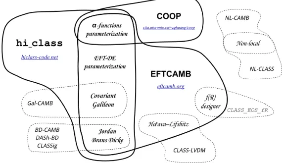
The codes used in this comparison, along with the models tested, are summarized in Fig. 1 and TableI and the details of each code can be found in the following sections.
A. EFTCAMB
EFTCAMB is an implementation [18,91] of the EFT of dark energy into the CAMB [9] EB solver (coded in FORTRAN90) which evolves the full set of perturbations (in the synchronous gauge) arising from the action in Eq.(4), after a built in module checks for the stability of the model under consideration. The latter includes conditions for the
avoidance of ghost and gradient instabilities (both on the scalar and tensor sector), well posedness of the scalar field equation of motion and prevention of exponential growth of DE perturbations. It can treat specific models (such as, Jordan-Brans-Dicke, designer-fðRÞ, Hu-Sawicki f(R), Hoˇrava-Lifshitz gravity, Covariant Galileon, and quintes-sence) through an appropriate choice of the EFT functions. It also accepts phenomenological choices for the time depend-ence of the EFT functions and of the dark energy equation of state which may not be associated to specific theories.
EFTCAMB has been used to place constraints on fðRÞ gravity[70], Hoˇrava-Lifshitz[38]and specific dark energy models[91]. It has also been used to explore the interplay FIG. 1. Overlap between codes and theories used in the comparison. Each code is represented by a silhouette that covers the models for which it has been compared. General-purpose and publicly available codes are represented by thick solid regions, while model-specific or private codes are enclosed by dashed lines. Note that we only show the models used in this paper, not the full theory space available to each code.
TABLE I. We show schematically the codes used in this comparison along with the models tested. This table provides the same information as Fig.1but in a different way. Note that we only show the models used in this paper, not the full theory space available to each code.
α Parametrization
EFT
Parametrization JBD
Covariant Galileon
f(R) designer
Hoˇrava Lifshitz
Non-Local Gravity
EFTCAMB ✓ ✓ ✓ ✓ ✓ ✓ ✗
hi_class ✓ ✓ ✓ ✓ ✗ ✗ ✗
COOP ✓ ✗ ✗ ✗ ✗ ✗ ✗
GalCAMB ✗ ✗ ✗ ✓ ✗ ✗ ✗
BD-CAMB ✗ ✗ ✓ ✗ ✗ ✗ ✗
DashBD ✗ ✗ ✓ ✗ ✗ ✗ ✗
CLASSig ✗ ✗ ✓ ✗ ✗ ✗ ✗
CLASS_EOS_fR ✗ ✗ ✗ ✗ ✓ ✗ ✗
CLASS-LVDM ✗ ✗ ✗ ✗ ✗ ✓ ✗
NL-CLASS ✗ ✗ ✗ ✗ ✗ ✗ ✓
between massive neutrinos and dark energy[92], the tension between the primary and weak lensing signal in CMB data
[93] as well as the form and impact of theoretical priors
[94,95]. An up to date implementation can be downloaded from http://eftcamb.org/. The JBD EFTCAMB solver is based on EFTCAMBOct15 version, while the others are based on the most recentEFTCAMBSep17version.
B.hi_class
hi_class (Horndeski in the Cosmic Linear Anisotropy Solving System) is an implementation of the evolution equations in terms of theαiðτÞ[19]as a series of patches to the CLASS EB solver [12,13] (coded in C). hi_class solves the modified gravity equations for Horndeski’s theory in the synchronous gauge (CLASS also incorporates the Newtonian gauge) starting in the radiation era, after checking conditions for the stability of the perturbations (both on the scalar and on the tensor sectors). Thehi_classcode has been used to place constraints on the αiðτÞ with current CMB data [96], study relativistic effects on ultra-large scales[97], forecast constraints with stage 4 clustering, lensing and CMB data [98] and con-straint Galileon gravity models[59].
The current public version ofhi_classis v1.1 [19]. The only difference between this version and the first one (v1.0) is that v1.1 incorporates all the parametrizations used in this paper. This guarantees that the results provided in this paper are valid also for v1.0. Lagrangian-based models, such as JBD and Galileons, are still in a private branch of the code and they will be released in the future. The hi_classcode is available fromwww.hiclass-code.net.
C. COOP
Cosmology Object Oriented Package (COOP) [99]is an Einstein-Boltzmann code that solves cosmological pertur-bations including very general deviations from theΛCDM model in terms of the EFT of dark energy parametrization
[26,28,32,100].
COOP assumes minimal coupling of all matter species and solves the linear cosmological perturbation equations in Newtonian gauge, obtained from the unitary gauge ones by a time transformationt→tþπ. For theΛCDM model, it solves the evolution equation of the spatial metric perturbation and the matter perturbation equations; details are given in Ref. [99]. Beyond the ΛCDM model, COOP additionally evolves the scalar field perturbationπ, using Eqs. (109)–(112) of Ref.[32]and verifying the absence of ghost and gradient instability along the evolution. Once the linear perturbations are solved, COOP computes CMB power spectra using a line-of-sight integral approach
[101,102]. Matter power spectra are computed via a gauge transformation from the Newtonian to the CDM rest-frame synchronous gauge.COOPincludes also the dynamics of the beyond Horndeski operator and has been used to study the signature of a non-zeroαHon the matter power spectrum as
well as on the primary and lensing CMB signals [103]. COOPv1.1 has been used for this comparison. The code and its documentation are available at www.cita.utoronto.ca/ ~zqhuang.
D. Jordan-Brans-Dicke solvers—modified CAMB and DASh
A systematic study, placing state of the art constraints on Jordan-Brans-Dicke gravity was presented in[20]using a modified version ofCAMBand an altogether different EB Solver—the Davis Anisotropy Shortcut Code (DASh)[10]. DAShwas initially written as a modification of CMBFAST
[7]by separating out the computation of the radiation and matter transfer functions from the computation of the line-of-sight integral. The code in its initial version, precom-puted and stored the radiation and matter transfer functions on a grid so that any model was subsequently calculated fast via interpolation between the grid points, supplemented with a number of analytic estimates and fitting functions that speed up the calculation without significant loss of accuracy. Such a speedup allowed the efficient traversal of large multidimensional parameter spaces with MCMC methods and made the study of models containing such a large parameter space possible[104–106].
The use of a grid and semianalytic techniques was abandoned in later, not publicly available versions of DASh, which returned to the traditional line-of-sight approach of other Boltzmann solvers. It is possible to solve the evolution equations in both synchronous and Newtonian gauge and therefore is amenable to a robust internal validation of the evolution algorithm. Over the last few years a number of gravitational theories, such as the tensor-vector-scalar theory [107,108] and the Eddington-Born-Infeld theory[109], have been incorporated into the code and has been recently used for cross-checks withCLASSin an extensive study of generalized dark matter[110,111].
In[20], the authors used the internal consistency checks withinDASh and the cross checks between DASh and a modified version of CAMB to calibrate and validate their results. We will use their modifiedCAMBcode as the baseline against which to compare EFTCAMB, hi_class, and CLASSig.
E. Jordan-Brans-Dicke solvers—CLASSig
standard kinetic term. CLASSig implements linear fluc-tuations either in the synchronous and in the longitudinal gauge (although only the synchronous version is main-tained updated with CLASS). The implementation and results of the evolution of linear fluctuations has been checked against the quasi-static approximation valid for sub-Hubble scales during the matter dominated stage
[112,113]. In its original version, the code implements as a boundary condition the consistency between the effective gravitational strength in the Einstein equations at present and the one measured in a Cavendish-like experiment (γσ20¼ ð1þ8γÞ=ð1þ6γÞ=ð8πGÞ, being G¼ 6.67×10⁻⁸cm3g−1s−2 the Newton constant) by tuning the potential. For the current comparison, we instead fix as initial condition γσ2ða¼10−15Þ ¼1;σ_ða¼10−15Þ ¼0 consistently with the choice used in this paper.
F. Covariant Galileon—modifiedCAMB
A modified version ofCAMBto follow the cosmology of the Galileon models was developed in [23], and sub-sequently used in cosmological constraints in [54,114]. The code structure is exactly as in default CAMB (gauge conventions, line-of-sight integration methods, etc.), but with the relevant physical quantities modified to include the effect of the scalar field. At the background level, this includes modifying the expansion rate to be that of the Galileon model: this may involve numerically solving for the background evolution, or using the analytic formulas of the so-called tracker evolution (see Sec.II D). At the linear perturbations level, the modifications entail the addition of the Galileon contribution to the perturbed total energy-momentum tensor. More precisely, one works out the density perturbation, heat flux, and anisotropic stress of the scalar field, and appropriately adds these contributions to the corresponding variables in default CAMB (due to the gauge choices in CAMB, one does not need to include the pressure perturbation; see [23] for the derivation of the perturbed energy momentum tensor of the Galileon field). In addition to these modifications to the default CAMB variables, in the code one also defines two extra variables to store the evolution of the first and second derivatives of the Galileon field perturbation, which are solved for with the aid of the equation of motion of the scalar field, and enter the determination of the perturbed energy-momentum tensor. Before solving for the pertur-bations, the code first performs internal stability checks for the absence of ghost and Laplace instabilities, both in the scalar and tensor sectors.
We refer the reader to [23] for more details about the model equations as they are used in this modified version of CAMB. While the latter is not publicly available,9 we
will use this EB solver to compare codes for this class of models.
G. f(R) gravity code—CLASS_EOS_fR
CLASS_EOS_fR implements the equation of state approach (EoS) [71,115,116] into the CLASS EB solver
[13]for a designerfðRÞmodel. In the EoS approach, the fðRÞmodifications to gravity are recast as an effective dark energy fluid at both the homogeneous and inhomogeneous (linear perturbation) level.
The d.o.f. of the perturbed dark-sector are the gauge-invariant overdensity and velocity fields, as described in detail in [72]. These obey a system of two coupled first-order differential equations, which involve the expressions of the gauge-invariant dark-sector anisotropic stress, Πde, and entropy perturbation, Γde. The expansion of Πde and Γde in terms of the other fluid d.o.f. (including matter) constitute the equations of state at the perturbed level. They are the key quantities of the EoS approach.
The fðRÞ modifications to gravity manifest themselves in the coefficients that appear in the expressions ofΠdeand Γde in front of the perturbed fluid d.o.f., see[72] for the exact expressions. At the numerical level, the advantage of this procedure is that the implementation of fðRÞ mod-ifications to gravity reduces to the addition of two first-order differential equations to the chosen EB code (e.g., CLASS), while none of the other pre-existing equations of motion, for the matter d.o.f. and gravitational potential, needs to be directly modified since it receives automatically the contribution of the total stress-energy tensor. In the code CLASS_EOS_fR, the effective-dark-energy fluid pertur-bations are solved from a fixed initial time up to present— the initial time being chosen so that dark energy is negligible compared to matter and radiation.
At this stage, the codeCLASS_EOS_fRis operational for fðRÞ models in both the synchronous and conformal Newtonian gauge. It shall soon be extended to other main classes of models such as Horndeski and Einstein-Aether theories.
A dedicated paper with details of the implementation and theoretical results and discussion is in preparation[117].
H. Horava-Lifshitz gravity codeˇ CLASS-LVDM
This code was developed in order to test the model of dark matter with Lorentz violation (LV) proposed in Ref. [82]. The code is based on the CLASS code v1.7, and solves the Eqs. (16)–(23) of Ref.[79]. The absence of instabilities is achieved by a proper choice of the param-eters of LV in gravity and dark matter. All the calculations are performed in the synchronous gauge, and if needed, the results can be easily transformed into the Newtonian gauge. Further details on the numerical procedure can be found in Ref.[84]where a similar model was studied. The code is available at http://github.com/Michalychforever/ CLASS_LVDM.
Compared to the standardCLASScode, one has to addi-tionally specify four new parameters:α,β,λ—parameters of LV in gravity in the khronometric model, described in Sec.II F, andY—the parameter controlling the strength of LV in dark matter. For the purposes of this paper we switch off the latter by putting Y≡0 and focus only on the gravitational part of khronometric/Horava-Lifshitz gravity.ˇ The details of differences in the implementation with respect toEFTCAMB can be found in AppendixD.
I. Nonlocal gravity—modifiedCAMB and CLASS
We compare two EB codes, a modified version ofCAMB and a modified version of CLASS, that compute the cosmology of a specific model of nonlocal gravity modi-fying the Einstein-Hilbert action by a term∼m2R□−2R(see Sec. IV Dfor details).
The modified version ofCAMB10 was developed by the authors of theGalCAMBcode, and as a result, the strategy behind the code implementation is in all similar to that already described in Sec.III Ffor the Galileon model. The strategy and specific equations used for modifying CLASS11 are outlined in details in Appendix A of[88]to which we refer the reader for an exhaustive account. In both cases, the equations that end up being coded are those obtained from the localized version of the theory that features two dynamical auxiliary scalar fields (see Sec.II G). Within both versions, the background evolution is obtained numerically by solving the system comprising the modified Friedmann equations together with the differential equations that govern the evolution of the additional scalar fields. Both implementa-tions include a trial-and-error search of the free parameterm of the model to yield a spatially flat Universe. At the perturbations level, one works out the perturbed energy-momentum tensor of the latter, and then appropriately adds the corresponding contribution to the relevant variables in the defaultCAMBcode, whereas these have been directly put into the linearized Einstein equations in theCLASSversion. The resulting equations depend on the perturbed auxiliary fields, as well as their time derivatives, which are solved for with the aid of the equations of motion of the scalar fields. The modified CAMB code was used in [89] to display typical signatures in the CMB temperature power spectrum (although[89]focuses more on aspects of nonlinear structure formation), whereas the modified CLASS one was used in various observational constraints studies[88,119,120].
IV. TESTS
In this section we present the tests that we have performed to compare the codes described in the previous section. Ideally one should compare codes for a wide range
of both gravitational and cosmological parameters. If one is to be thorough, this approach can be prohibitive computa-tionally. Furthermore, that is not the way code comparisons have been undertaken in other situations. In practice one chooses a small selection of models and compares the various observables in these cases. This was the approach taken in the original EB code comparisons[8]but is also used in, for example, comparisons between N-body codes forΛCDM simulations as well as modified gravity theories
[24]. Therefore, we will follow this approach here: for each theory we will compare different codes for a handful of different parameters.
A crucial feature of the comparisons undertaken in this section is that they always involve at least a comparison between a modifiedCAMBand a modifiedCLASSEB solver. This means that we are comparing codes which, at their core, are very different in architecture, language and genesis. For the majority of cases, we will use EFTCAMB and hi_class as the main representatives for either CAMBorCLASSbut in one case (nonlocal gravity) we will compare two independent codes. Another aspect of our comparison is that at least one of the codes for each model is (or will shortly be made) publicly available.
In our comparisons, we will be aiming for agreement between codes—up tol¼3000for the CMB spectra and k¼10hMpc−1 in the matter power spectrum—such that the relative distance between observables is of order 0.1%, with the exception of low-multipoles (l<100) where we accept differences up to 0.5% since these scales are cosmic variance limited. We consider this as a good agreement, since it is smaller than the cosmic variance limit out to the smallest scales considered, i.e., 0.1% atl¼3000 in the most stringent scenario (see, e.g.,[8]). We shall see that for
l≲300in the EEspectra the relative difference between codes exceeds the 1% bound. This clearly evades our target agreement, but it is not worrisome. Indeed, on those scales the data are noise dominated and the cosmic variance is larger than 1%. It is important to stress here that all the relative differences shown in the following figures are expressed in½%units, with the exception ofδCTE
l . Since CTE
l crosses zero, we decided not to use it and to show the simple difference in½μK2 units instead.
Another crucial aspect has been the calibration of the codes. To do so, we fixed the precision parameters so that all the tests of the following sections (i) had at least the target agreement, and (ii) the speed of each run was still fast enough for MCMC parameter estimation. While the first condition was explained in the previous paragraph, for the latter we established a factor 3–4 as the maximum speed loss with respect to the same model run with standard precision parameters. This factor is a rough estimate that assumes that in the next years the CPU speed will increase, but even with the present computing power MCMC analysis with these calibrated codes is already possible. It is important to stress that most of the increased precision parameters are necessary 10This version of the
CAMBcode for theRRmodel is not publicly available, but it will be shared by the authors upon request.
only to improve the agreement in the lensing CMB spectra on small scales, which is by default 1–2 orders of magnitude worse than the other spectra.
We will be parsimonious in the presentation of results. As will become clear, we have undertaken a large number of cross-comparisons and it would be cumbersome to present countless plots (or tables). Therefore, we will limit ourselves to showing a few significant plots that help us illustrate the level of agreement we are obtaining and spell
out, in the text, the battery of tests that were undertaken for each class of models. We have found our results (i.e., the precision with which codes agree) to be relatively insensi-tive to variations of the cosmological parameters.
Before showing the results of our tests, it is useful to stress here that all the precision parameters used by the codes to generate these figures are specified in AppendixC, while the cosmological parameters for each model are reported in AppendixB.
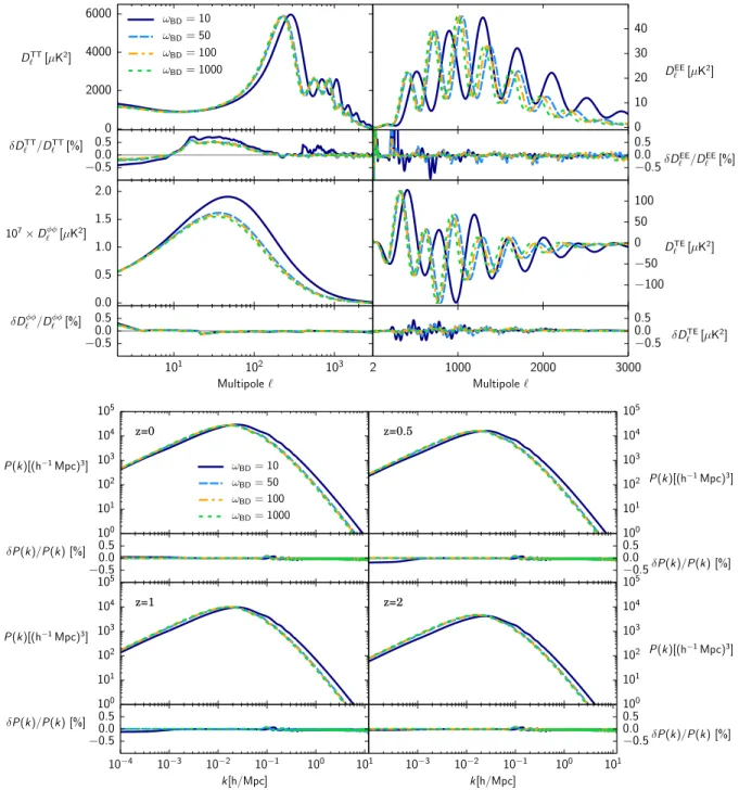
FIG. 2. JBD. Top figure: TheTT,EE, lensing andTEangular power spectra of the CMB—withDXY
A. Jordan-Brans-Dicke gravity
We have validated the EFTCAMB, hi_class, and CLASSig EB Solvers in two steps. We have first used DASh and the modified camb of[20]to validateEFTCAMB with particular caveats. The current implementation of DASh uses an older version of the recombination module RECFAST—specificallyRECFAST1.2. We have runEFTCAMB with this older recombination module and found that the agreement with DASh is at the sub-percent level. We have confirmed that this is also true in a comparison between EFTCAMB and the modified CAMB of [20]. We note the codes of [20] have only been cross checked and calibrated out to l¼2000 and for a maximum wavenumber kmax¼0.5hMpc−1. With the more restricted cross check of the first step in hand, we have then comparedEFTCAMB,hi_class, andCLASSigwith the more up to date recombination module—specifically RECFAST1.5—and out to largelandk. There are two main effects on the perturbation spectrum in JBD gravity: the effect of the scalar field on the background expansion and the interaction of scalar field fluctuations with the other perturbed fields.
In Fig.2we showClandPðkÞfor a few different values ofωBD(see AppendixB 1for the cosmological parameters used in this figures) as well as the relative difference for these quantities between hi_class and EFTCAMB. We can clearly see a remarkable agreement between the codes, well within what is required for current and future precision analysis. It is possible to notice that for l≲102 the disagreement in the temperature Cl increases for all the models up to ≃0.5%. As we shall see, this is a common feature when comparing aCAMB-based code with aCLASS -based code, and it is present even for ΛCDM, i.e., using CAMB and CLASS instead of our modified versions (see, e.g., Fig.6). Moreover, it has been checked that forΛCDM a systematic bias of 1-2 orders of magnitude smaller than the cosmic variance at l<100does not affect parameter extraction with present data, see Sec. II of[1]. Therefore, even if this issue deserves further investigation for DE/MG models, we believe that a better agreement at those scales is beyond the scope of this paper. The other issue of Fig.2, common to all the models we show in this paper, is that the disagreement in theCEE
l on very large scales exceeds the 1% bound. As we already mentioned, this is due to the fact that their amplitude approaches zero and then the relative difference is artificially boosted. This is not to worry, since (i) the amplitude of the polarization angular power spec-trum is very small on large scales with respect to small scales and (ii) we are protected by cosmic variance. Finally, note that the agreement holds even for extremely small values of ωJBD; this is essential if these codes are to be accurately incorporated into any Monte Carlo parameter estimation algorithm.
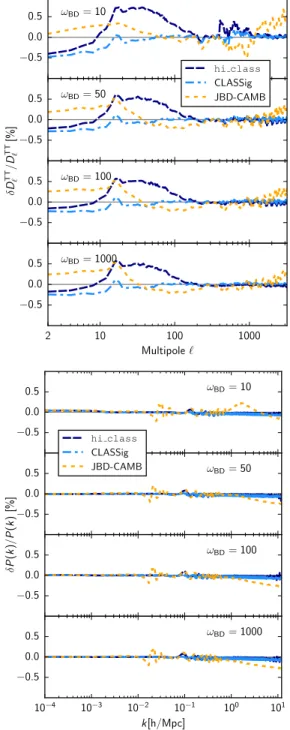
Similar results can be found in Fig.3, where we compare the outputs of BD-CAMB,CLASSig, andhi_class(for
reference) with the outputs generated by EFTCAMB. For simplicity, we show the result only for CTT
l andPðkÞ at z¼0, but the other spectra have similar behaviour as in Fig.2. It is possible to note that the level of agreement is well within the 1% requirement for all the codes, validating their outputs even in “extreme” regions of the param-eter space.
This is an important first cross check between EB solvers. JBD is a canonical theory, widely studied in many regimes, and at the core of many scalar-tensor theories. It is a simple model to look at in that the background is monotonic and that only a very small subset of gravitational parameters are nontrivial.
B. Covariant Galileons
The covariant Galileon theory has been implemented in the current version ofhi_classandEFTCAMB. Both
these codes were compared against the modified CAMB described in Sec.III F, i.e.,GALCAMB. The differences in the implementation are that EFTCAMB and GALCAMB assume the attractor solution for the evolution of the background scalar field, while hi_class evolves the full background equations with the possibility of having arbitrary initial conditions. For comparison with other codes, in hi_class we will set the initial conditions for the background scalar field as if it were on the attractor, to make the two approaches consistent and
comparable. As explained in Sec. II D, and unlike in the JBD case (which is not self-accelerating), there is no extra parameter to vary in the case of the cubic Galileon. Once one is on the attractor and one chooses the matter densities, the evolution is completely pinned down. On the contrary, for the quartic and quintic Galileon models, there are one (for the quartic) or two (for the quintic) additional parameters. This implies that care should be had in enforcing the stability conditions (i.e., enforcing ghost-free backgrounds or preventing the existence of gradient instabilities).
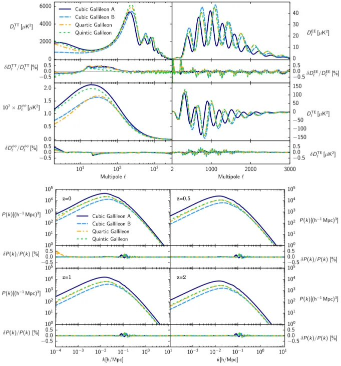
In Fig.4it is possible to see the CMB angular power spectra and the matter power spectrum at different redshifts for two cubic Galileon models, one quartic and one quintic. While the exact values for the parameters used for this comparison are shown in Appendix B 2, here it is important to stress that all these models have been chosen to be bad fits to current CMB and expansion history data. From these figures it can be seen that hi_class and EFTCAMB agree to within the required precision. We have checked that they are also completely consistent withGALCAMB, as it is possible to see in Fig. 5, where we show the comparison between hi_class and GALCAMB. As in the case of JBD, we have varied the cosmological and gravitational parameters and found that this agree-ment is robust.
C. f(R) gravity
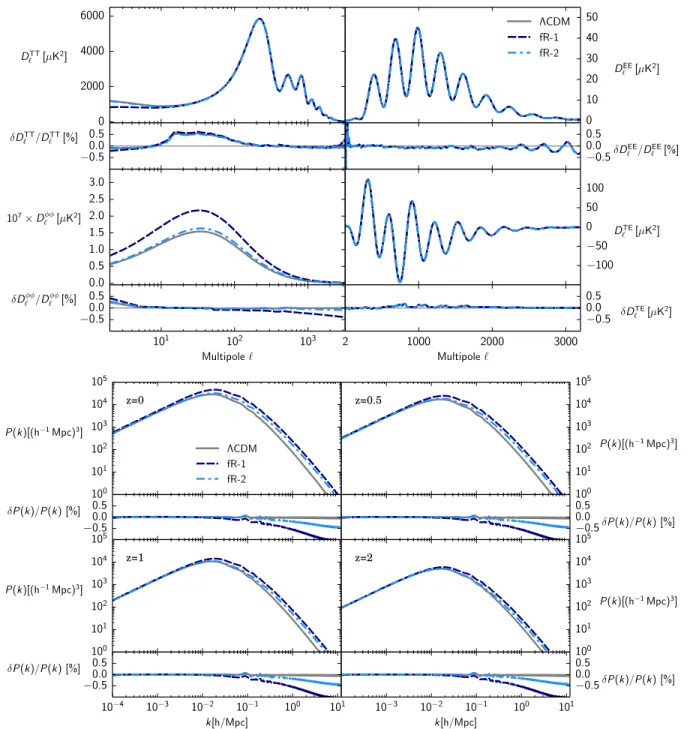
fðRÞ gravity has been implemented in both EFTCAMB and CLASS_EOS_fR following two independent approaches.12 We focus on designer fðRÞ models that result in a ΛCDM expansion history and differ from GR at the perturbation level, displaying an enhancement of small scale structure clustering. Once the expansion history has been chosen one has to fix a residual parameter B0, corresponding to the present value of B, as in Eq.(22). We focus on two different values of theB0 parameter: at first we compare cosmological predictions for B0¼1, a value that has already been excluded by experiments, to make sure no difference between the two codes is hidden by the choice of a small parameter; we then focus onB0¼0.01, that is at the boundary of CMB only experimental constraints [91,92]and in the range of interest for N-body simulations. In Fig.6 it is possible to see that all compared spectra agree within the required precision. Discrepancies in all CMB spectra are consis-tent with the comparison to other codes and within 0.5%. As in the previous cases, we have varied cosmological and gravitational parameters and found that agreement is robust. The matter power spectrum comparison shows
some residual difference that reaches approximately 1% on very small scales, k¼10h=Mpc, for large values of the free parameter, B0¼1. The latter value is already largely excluded by CMB only data, and the scales involved are affected by nonlinear clustering, hence this discrepancy is not worrisome.
FIG. 5. Covariant Galileons. Top figure: The relative difference of theTT, EE, lensing, and TE angular power spectra of the CMB for the same models showed in Fig.4betweenGALCAMB and hi_class (we find the same level of agreement with EFTCAMB). Bottom figure: The same as in the top figure but for the matter power spectrum at different redshifts.
D. Nonlocal gravity
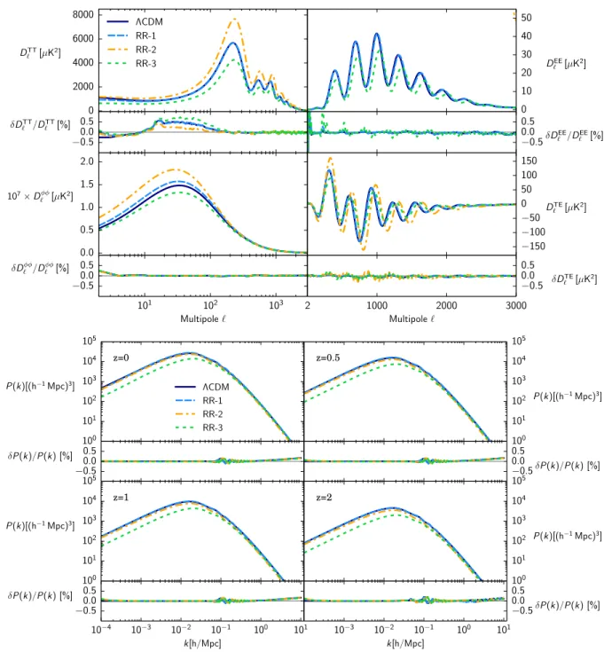
For the comparison of the two EB solvers of the non-localRRmodel, we have considered three sets of cosmo-logical parameters values, shown in AppendixB 4. Two of them are markedly poor fits to the data [RR-2andRR-3in Fig. 7, but the other gets closer to what is allowed observationally (called RR-1 here)]. In Fig. 7, the ΛCDM predictions shown correspond to the same param-eters values as RR-1. Recall, the ΛCDM andRR models
have the same number of free parameters. The correspond-ing figures show that the level of agreement between these two EB solvers meets the required standards for all spectra, scales, and redshifts shown. In fact, the shape of the relative difference curves are similar in betweenΛCDM and theRR models, which suggests that the observed differences (small as they are) are mostly due to intrinsic differences in the default codes (CAMB and CLASS), and less so due to the modifications themselves.
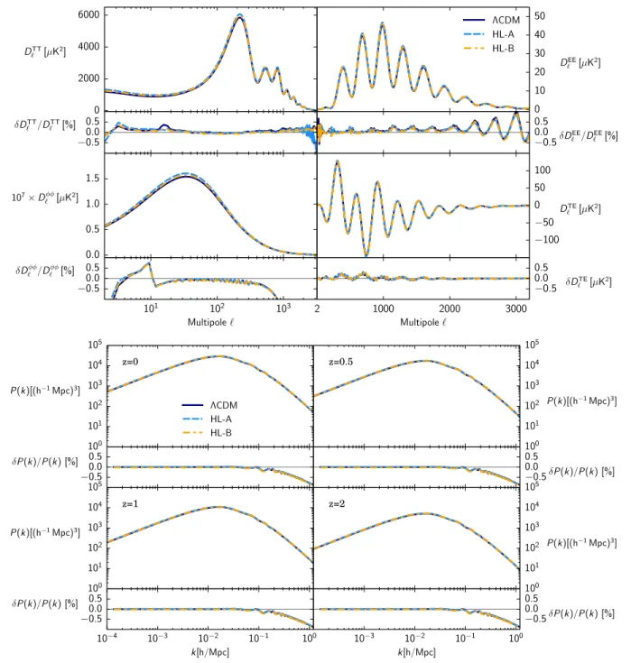
E. Horava-Lifshitz gravityˇ
We now proceed in validating EFTCAMB and CLASS -LVDMfor Hoˇrava-Lifshitz gravity. Because of the different implementation of the background solver (see AppendixD
for details), we have limited the comparison to the subset of parameters satisfying the condition Gcosmo¼GN, elimi-nating all the differences arising from it. In the top panels of
that this difference is not a peculiarity of the MG model, but it is already present at the ΛCDM level (blue line). The differences at large-lare common to all the models under investigation. As for the discrepancy at low-l, the fact that it is present even forΛCDM suggests that it is caused by an inaccuracy inCLASSv1.7, whichCLASS-LVDMis based on, and not by the modification itself. Indeed, one may observe that this issue is absent inhi_classbased on an updated
code (v1.7). For illustrative purposes we decided to cut the matter power spectrum at the value k¼1hMpc−1. It should be pointed out that the scales k≳0.1hMpc−1 are significantly affected by nonlinear clustering, therefore the output of linear Boltzmann codes in this region is of little practical value.
Note that we used the standard CLASS accuracy flags except for lensing, where a more accurate mode has been employed by imposing accuratelensing¼TRUE.
F. Parametrized Horndeski functions
Up to this point we have considered a specific set of theories which, albeit representative, only involve a very restricted set of possible time evolution for either the Horndeski or EFT functions. This means that either some of the free functions are set to zero or a lower dimensional subspace of the full function space is explored [see Eq. (11) for a good example]. We now need to explore a wider choice of theories and time evolutions.
Ideally, we should somehow explore and compare the full parameter space described by the time dependent functions fαiðτÞ; wDEðτÞg. This is obviously impossible, but also unnecessary for our purposes. Indeed, the only modifications introduced by COOP, EFTCAMB, and hi_classare at the level of the Einstein and scalar field equations. Therefore, it is sufficient to use a parametriza-tion that is capable of capturing all the terms present there. Checking that for particular parametrizations, such as rapidly varying time dependent functions, the three codes agree would in practice correspond to a check on the differential equations solvers of each code, and this is beyond the scope of this work.
The guiding principle in choosing a particular para-metrization has been to recover standard gravity at early times, to preserve the physics of the CMB and to ensure a quasi-standard evolution until recent times, i.e., approx-imately until the onset of dark energy. For example a parametrization closely related with this principle, which has been used in both data analysis[96]and forecasts[98], takes the form
wDE¼w0þ ð1−aÞwa
αi¼ciΩDE: ð38Þ
Even if this parametrization is capable of turning on all the possible freedom of Horndeski theories up to linear level, it may be not sufficient. Indeed, the system of equations for the evolution of the perturbations contains bothfαiðτÞ; wDEðτÞg and their time derivatives. Thus, we have extended this parametrization to be able to modulate the magnitude of the derivatives of these functions. The simplest choice is then
wDE¼w0þ ð1−aÞwa
M2¼1þδM20aη0
αi¼α0iaηi; ð39Þ
where i stands for K, B, T. The translation from the αi functions to the EFT functions is provided in Appendix A.
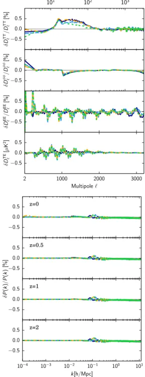
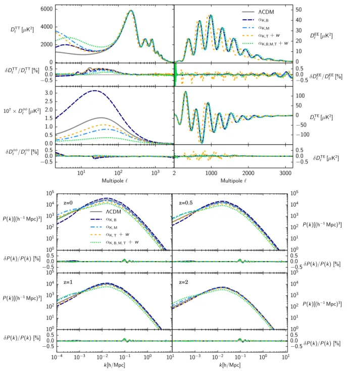
In Fig. 9, we show the lensed temperature Cl and the matter power spectrumPðkÞcalculated at different redshifts for few different values offw0; wag,δM20, α0i andηi (see AppendixB 6 for the list of values used in this compari-son). The cosmological parameters are the same for each curve in the plots. The models shown in the figures were built so as to isolate the effect of eachαi. Considering the fact thatαK andαT alone are known to have a small effect on the observables, e.g.,[27,34,96,98,121], we have always combined them with other functions (eitherαiorwDE). The
αK;B;M;Tþw model (green dotted line) contains all the possible modifications that a Horndeski-like theory can produce. We should stress that the values used here were chosen specifically to have large deviations with respect to the referenceΛCDM model and with respect to each other. During the comparison process many more models were explored, both close to ΛCDM and unrealistically far from it.
An additional requirement to accept models for this comparison was that they were not sensitive to the specific initial conditions (ICs) set for the perturbations: The codes are set up to start with and evolve superhorizon adiabatic ICs, as predicted by standard inflation. Typically, in models which go back to GR quickly enough at early times, the other, isocurvature, modes decay with respect to the adiabatic mode, so it is irrelevant what the initial condition for the scalar field is, since it will reach the required adiabatic mode quickly.
However there are situations, typically when the modi-fication of gravity does not decrease rapidly enough to the past, in which the isocurvature modes do not decay quickly enough (or even grow), and then it is very important that the correct, or at least equivalent, ICs be chosen.
The codes currently have different methods of setting ICs, which is irrelevant when the isocurvature modes decay rapidly enough, but can be important when they are not. We thus have to ensure that we are in a situation where the adiabatic ICs are an attractor for perturbations during radiation domination. The issue of setting the correct ICs for dark-energy perturbations is still an open problem and it will be addressed in future versions of the codes under consideration.
αK;B;M;Tþw models have relative differences slightly larger than the other models for the EE and TE CMB spectra. While it is difficult to identify one of theαiorwas the responsible for these deviations, we found that improv-ing the precision parameters of each code solves this issue. This indicates that these two models are particularly com-plicated and they need increased precision parameters to reach the agreement of the other models. For this particular
parametrization, a third code has been tested, i.e.,COOP. The agreement betweenCOOPandEFTCAMBis shown in Fig.10. It can be noted that, even if the relative differences in CMB spectra remain below the 1% level, they blow up in the matter power spectrum up to 2–3% on small scales. This seems to be an effect of the accuracy of COOP. Indeed, while COOPis calibrated to get a good agreement on large scales, it lacks of precision fork≳1hMpc−1.
FIG. 9. Alphas. Top figure: TheTT,EE, lensing, andTEangular power spectra of the CMB for a referenceΛCDM and four different choices of thefwDE;αigfunctions along with the relative difference betweenEFTCAMBandhi_class. Bottom figure: The same as in