On Weak Solvability of Boundary Value Problems for Elliptic Systems

Revista Colombiana de Matem´aticas Volumen 47(2013)2, p´aginas 191-204

On Weak Solvability of Boundary Value

Problems for Elliptic Systems

Sobre la solubilidad d´ebil de problemas con valores en la frontera para sistemas el´ıpticos

Felipe Ponce

,

Leonid Lebedev

,

Leonardo Rend´

on

Universidad Nacional de Colombia, Bogot´

a, Colombia

Abstract.This paper concerns with existence and uniqueness of a weak so-lution for elliptic systems of partial differential equations with mixed bound-ary conditions. The proof is based on establishing the coerciveness of bilin-ear forms, related with the system of equations, which depend on first-order derivatives of vector functions in_Rn_{. The condition of coerciveness relates to}

Korn’s type inequalities. The result is illustrated by an example of boundary value problems for a class of elliptic equations including the equations of linear elasticity.

Key words and phrases. Weak solvability, Boundary value problems, Elliptic equations, Korn’s type inequality.

2010 Mathematics Subject Classification.35J57, 74G65.

Resumen.Este art´ıculo trata sobre la existencia y unicidad de una soluci´on d´ebil para sistemas el´ıpticos de ecuaciones diferenciales parciales con condi-ciones de frontera mixtas. La demostraci´on se basa en la determinaci´on de la coercividad de formas bilineales, relacionadas con el sistema de ecuaciones, las cuales dependen de las derivadas de primer orden de funciones vectoriales enRn. La condici´on de coercividad se relaciona con desigualdades tipo Korn. El resultado se ilustra mediante un ejemplo de problemas con valores en la frontera para una clase de ecuaciones el´ıpticas, incluyendo las ecuaciones de elasticidad lineal.

Palabras y frases clave. Solubilidad d´ebil, problemas con valores en la frontera, ecuaciones el´ıpticas, desigualdad tipo Korn.

1. Introduction

Systems of elliptic partial differential equations arise frequently in problems of continuum mechanics. To formulate boundary value problems (BVPs), we should supply the equations with some boundary conditions. We will consider the linear partial differential equations derived from an energy type functional. We will get solutions to a BVP minimizing the energy type functional. Such a solution will be called weak. As we expect to apply the results to physical problems we use the terminology like “energy”, “displacements”, etc.

In general case solution of a BVP will be reduced to the minimization problem for a functional of the formE(u) = 1

2B(u, u)−f(u) in a Hilbert space

H, whereB is a symmetric bilinear form andf is a linear functional inH. It is well know that

Theorem 1.1 ([15, 16]). Let B be a continuous symmetric bilinear form in a Hilbert spaceH. Iff is a continuous linear functional andB(u, u)≥Ckuk2_for

every u∈H and some constant C >0, then E attains a unique minimum in

H. Furthermore,u0 is the minimum point if and only if it is a unique solution

to equation

B(u0, v) =f(v) (1)

for every v∈H.

This simple result allows us to prove existence–uniqueness theorems for mechanical problems; it motivates the following definition.

Definition 1.2. A bilinear formB in a Hilbert space is coercive ifB(u, u)≥

Ckuk2_{for every u∈H and some constantC.}

In the proof of existence and uniqueness of weak solutions of the problems under consideration, the most troublesome point is to establish the coerciveness ofB. In linear elasticity such coerciveness is also called Korn’s inequality which was first proved in [13, 14]. Subsequent generalizations of Korn’s inequality can be found in [9, 5, 17, 11, 6, 1]. One of the most important latest papers on Korn’s inequality is due to V. A. Kondrat’ev and O. A. Oleynik [12], where it is established in a general form.

Similar problems frequently arise in equilibrium or stationary linear bound-ary value physical problems [3, 4, 7, 8, 10]. We extend some known results for linear elasticity to a general case and consider a general coerciveness problem of B, construction of abstract energy spaces related to B as well as the weak setup of corresponding boundary value problems and their solvability.

Assume that Ω is a connected bounded open set in _Rn _{with piecewiseC}1

boundary ∂Ω. LetB be a positive bilinear form, that is, ifB u,u

=0for a smooth vector function u : Ω⊂_Rn _→

Rn, such that u|Γ =0 for some open

valid. The linear space of smooth functions withu|Γ =0constitutes an inner

product space if we takeB u,v

as an inner product. Completion of this space with respect to the norm induced by the inner product is an energy space.

The bilinear form used for the inner product is

B u,v

=

Z

Ω

m

X

i,j=1

aij(x)Li ∇u,u, xLj ∇v,v, xdx (2)

where aij _{∈ L}∞_{(Ω) are components of a symmetric positive definite matrix}

and the linear formsLi are

Li ∇u,u, x

= n

X

k,l=1

bkli (x)∂kul+ n

X

k=1

cki(x)uk.

Let f : Ω ⊂ Rn → Rn and g : ∂Ω−Γ → Rn be vector functions, these

define the energy functional

E u=1 2B u,u

−

Z

Ω

f

·

Z

∂Ω−Γ

g

·

By analogy with elasticity equations, we presentB in the form

B u,v

=

Z

Ω

X

t

"

−X

k,s

∂s

X

l

dklst∂kul+qkstuk

!

+X k,l

qtkl∂kul+

X

k

pktuk

#

vtdx+

Z

∂Ω−Γ

X

t

" X

k,l,s

dklst∂kulns+

X

k,s

qkstukns

#

vtdS,

where dS is the surface area element,nthe normal vector to the surface and the coefficients are

dklst=X i,j

aijbkl_i bst_j , qkst=X i,j

aijck_ibst_j, pkt=X i,j

aijck_ict_j.

If the functions involved inEare sufficiently smooth and satisfy the bound-ary condition, functionalEcan be obtained from (2) integrating by parts. Us-ing standard methods of calculus of variations, assumUs-ing existence of a smooth minimizeruofE and minimizingE over the set of smooth functions equal to zero on Γ, we get the corresponding system of partial differential equations

−X

k,s

∂s

X

l

dklst∂kul+qkstuk

!

+X k,l

qtkl∂kul+

X

k

fort= 1, . . . , n. Moreover, on∂Ω−Γ we obtain the natural condition

X

k,s

X

l

dklst∂kul+qkstuk

!

ns=gt (5)

for t = 1, . . . , n, that is analogous to Neumann’s condition for the Laplace equation, whereas on Γ we have Dirichlet condition

u|Γ= 0. (6)

Definition 1.3. A vector function u is a weak solution of the system in (4) with boundary conditions (5) and (6) if it is a minimum point of the energy functional E u

in (3).

We will present some sufficient conditions for coerciveness and continuity ofB in the Hilbert space Hof vector functions in W1,2(Ω)n with zero trace value in Γ ⊂ ∂Ω. In this way we will show that the energy norm B u,u12 is an equivalent norm inH, which in turn insure existence and uniqueness of a weak solution of the boundary value problem (4)–(6) in the space H. We apply this result to a particular type of bilinear forms, generalizing a result from the theory of shallow shells [18] and consider an example of boundary value problems for a class of elliptic equations including the equations of linear elasticity.

Notation. The norm of a vector fieldu in

Lq_(Ω)n

=Lq_{(Ω)× · · · ×L}q_(Ω) and theL2_{(Ω) norm of∇uare, respectively,}

kukq =

( Z

Ω

n

X

i=1 |ui|

q

)1q

and ∇u ₂=

( Z

Ω

n

X

i,j=1 |∂iuj|

2

dx

)12

.

The norm of

W1,2_(Ω)n

=W1,2_{(Ω)× · · · ×W}1,2_{(Ω) is} kuk1,2=

kuk2

2+k∇uk 2 2

1 2_.

2. Equivalence of Energy and Sobolev’s Norms

Let us rewrite the symmetric bilinear functional

B u,v

=

Z

Ω

m

X

i,j=1

aij(x)Li ∇u,u, xLj ∇v,v, xdx (7)

where aij

is a symmetric positive definite matrix almost everywhere (a.e.) and the linear formsLi are

Li ∇u,u, x= n

X

k,l=1

bkl_i (x)∂kul+ n

X

k=1

We can also write

Li ∇u,u, x

=Mi ∇u, x

+Ni u, x

,

whereMi andNi are linear forms. In what follows, we assume that

aij, bkl_i ∈L∞(Ω) (8)

ck_i ∈Lq(Ω) for n < q≤ ∞. (9) By the positive definiteness of aij

, there exists a positive bounded a.e. func-tionhsuch that

B u,u

≥

Z

Ω

m

X

i=1

h(x) Li ∇u,u, x

2

dx.

From this, it is easy to prove thatBis positive definite if and only ifLi ∇u,u, x= 0 a.e. for everyi implies thatu=0, a.e.

We will use the following classical properties of Sobolev spaces

Theorem 2.1 (The Embedding theorem [2]). Suppose that Ω is a bounded open set satisfying the cone condition. Then

(i) Ifn= 2,W1,2(Ω)is continuously and compactly embedded in Lq(Ω), for 1≤q <∞; that is, for every u∈W1,2_{(Ω), there exists a constantC such}

that kukq ≤Ckuk1,2 and if un * uinW1,2(Ω), thenun→0 inLq(Ω). (ii) If n >2,W1,2_{(Ω) is continuously embedded in L}q_{(Ω), for1 ≤q≤} 2n

n−2,

and compactly embedded in Lq_{(Ω), for 1≤q <} 2n n−2.

The continuous embedding is known as Sobolev embedding theorem, and the compact embedding as Rellich-Kondrachov theorem.

The goal of this section is to show that the termsMi, which include only first order derivatives, determine the equivalence of the energy norm with the Sobolev’s norm.

Theorem 2.2. If B is the bilinear form given by the Equation (7) and

Z

Ω

m

X

i,j=1

aij(x)Mi ∇u, xMj ∇u, xdx≥C

∇u

2

2, (10)

then the energy normB u,u12 _{is equivalent to the norm of H.}

Corollary 2.3. Suppose thatB satisfies the hypothesis of Theorem 2.2 and let

f ∈

Lp(Ω)n and g∈

Lp∗(∂Ω−Γ)n for 1< p, p∗≤ ∞, if n= 2,

f ∈hLn2+2n _(Ω)

in

and g∈hL2(nn−1)(∂Ω−Γ)

in

, if n >2.

Then for the corresponding boundary value problem (4)–(6)there exists a unique weak solution in H.

Proof. It is a consequence of Theorem 1.1 and the continuity of the functionals

R

Ωf

·

R

∂Ω−Γg

·

W1,2_(Ω)n

. X

Inequality (10) is of Korn’s type. The name comes from the classical Korn’s inequality in elasticity, which depends strongly on the fact that the vector field is zero on some open subset of the boundary

Z

Ω

n

X

i,j=1

(∂ivj+∂jvi)2dx≥Ck∇vk22.

Before proving Theorem 2.2, we need the following lemma.

Lemma 2.4. Suppose that Ω is a bounded open set satisfying the cone con-dition and Z⊂

W1,2_(Ω)n

is a closed subspace. Let B be a continuous posi-tive definite bilinear form in Z. If the conditions vk *0 in

W1,2(Ω)n and

B vk,vk→0 imply thatk∇vkk2→0, then

B v,v

≥Ckvk2

1,2 (11)

for some constant C.

Proof. Suppose contrarily that B v,v

≥ Ckvk2

1,2 is false for any C. Then

we can find a sequence

vk such that B vk,vk → 0 and kvkk1,2 = 1. As Z is a Hilbert space and

vk is bounded, we can assume that the sequence converges weakly to some vectorv0. AsB(

·

positive definiteness of B, 0≤B vk−v0,vk−v0

≤B vk,vk

−2B vk,v0

+B v0,v0

.

Taking the limit whenk→ ∞we get 0≤ −B(v0,v0).

So,B v0,v0= 0, which implies thatv0=0. Thusvk*0 inW1,2(Ω) n

. As

B vk,vk

→0. by the assumptions we conclude that∇vk

₂→0.

As vk * 0 in W1,2(Ω) n

, by Rellich–Kondrachov’s theorem we see that

vk→0 in

L2_(Ω)n

. Thusvk→0 in

W1,2_(Ω)n

, which contradicts the equal-ity vk

Proof of Theorem 2.2. To verify the continuity of the bilinear form B, by the symmetry of B it suffices to show thatB u,u

≤Ckuk2_1,2. Choosing p

according to (9) andqsuch that 1_p+1_q = 1₂, for the components of the bilinear form we have

Z Ω

aijbkli b st

j ∂kul∂sutdx

≤1 2 a ij

bkli b st j

_∞ k∂kulk22+k∂sutk22

≤C1

u

2

1,2, (12)

Z Ω

aijbkl_i cs_j∂kulusdx

≤ aijbkl_i

∞

cs_j

_pk∂kulk2kuskq ≤C2

u

2

1,2, (13)

Z Ω

aijck_ics_jukusdx

≤1 2 aij _∞ ck_i

2

pkukk

2

q+

cs_j

2

pkusk

2

q

≤C3

u

2

1,2. (14)

So we conclude thatB is continuous.

By Lemma 2.4, now we only need to prove thatuk *0 inW1,2(Ω) n

and

B uk,uk

→0 together imply that ∇uk

₂ →0. We write the bilinear form

as follows:

B uk,uk

= Z Ω m X i,j=1

aij(x)Mi ∇uk, x

Mj ∇uk, x

dx+ 2 Z Ω m X i,j=1

aij(x)Mi ∇uk, x

Nj uk, x

dx + Z Ω m X i,j=1

aij(x)Ni uk, xNj uk, xdx. (15)

By Rellich-Kondrachov’s theorem we know thatuk

_q → 0. The first

equality in (14) shows that the third term on the right-hand side of the In-equality (15) tends to zero. In a similar fashion, by the first inIn-equality in (13) and the boundedness ofk∂iuk,jk2, the second term also tends to zero. Thus, by

Equation (10), we get ∇uk

₂→0 ask→ ∞, which concludes the proof. X

When we try to prove the coerciveness of B, the uniform positive defi-niteness of aij

allows us to simplify the proof and to extend theorems on equivalence between energy norms and Sobolev’s norms.

Definition 2.5. The terms aij

are uniformly positive definite if m

X

i,j=1

aij(x)ξiξj ≥θ m

X

i=1

for every x∈Ω and some constantθ >0. This stronger requirement implies that

B u,u

≥θ

Z

Ω

m

X

i=1

Li ∇u,u, x

2

dx.

In general, it is easier to prove the coerciveness of the form in the right hand side, obtaining thus the coerciveness of the original bilinear form. Moreover, once it is proved that

b

B u,v

=

Z

Ω

m

X

i=1

Li ∇u,u, x

Li ∇v,v, x

dx (16)

is coercive, we can extend this result to a wider class of bilinear forms.

Theorem 2.6. Suppose that aij_(x)

is uniformly positive definite and

T(x) :_Rm→_Rm (vi)7→

m

X

t=1

tij(x)vj

!

(17)

is a non-singular linear operator at each point, such that T(x)−1

is bounded.

The bilinear form B defined by

Z

Ω

m

X

i,j=1

aij

m

X

t=1

tit(x)Lt ∇u,u, x

! m

X

t=1

tjt(x)Lt ∇v,v, x

!

dx (18)

is coercive if Bb in (16)is coercive.

Proof. By uniform coerciveness of aij, the theorem follows from the inequal-ity

m

X

i=1

m

X

j=1

tij(x)Lj ∇u,u, x

!2

≥C

m

X

i=1

Li ∇u,u, x

2

,

where C > 0 is a constant, after integrating over Ω. But this inequality is an easy consequence of

T(x)(v)

≥

1

T(x)−1

|v| ≥ 1

C1 |v|

where |

·

3. Generalization of a Bilinear Form in Elasticity

The following bilinear form is an extension of the body strain energy in theory of shallow shells,

B u,v

=

Z

Ω

n

X

i,j,k,l=1

aijkl(x)Lij ∇u,u, xLkl ∇v,v, xdx

where aijkl _=aklij _∈L∞_{(Ω) are uniformly positive definite, that is, for some}

θ >0 and everyx∈Ω we have n

X

i,j,k,l=1

aijkl(x)ξijξkl≥θ n

X

i,j=1

ξ2_ij.

The linear components are

Lij(v) =∂ivj+∂jvi+ckijvk whereck_ij ∈L∞(Ω).

By the uniform positive definiteness of aijkl

, instead ofB, we prove the coerciveness of

b

B(u,v) =

Z

Ω

n

X

i,j=1

Lij ∇u,u, x

Lij(∇v,v, x)dx.

As noted in the preceding section, by means of Theorem 2.6, we can extend equivalence of the energy norm B u,u12 _{to a greater class of energy norms.} Linear forms Lij can be considered as the components in the canonical basis of operator

L(v)=∇v+∇vT +C

·

where the components of C

·

kc k ijvk

. So we have the identity

b

B u,v

=

Z

Ω

trL(u)L(v)Tdx. (19)

An additional advantage of Bb is its invariance under orthogonal

transfor-mations. To see this, suppose {ei} is an orthonormal basis for Rn and let

ei0 = P

iq i

i0ei define a new orthonormal basis, whose inverse transformation is ei =Piq

i0

i ei0, whereP

j0q

j0

i qkj0 =δ_ik. As neither ∇v norC

·

particular basis and the trace of a matrix is invariant under orthogonal trans-formations, we have from Equation (19) that

Z Ω n X i,j=1

∂ivj+∂jvi+ n

X

k=1

ck_ijvk

2 dx= Z Ω0 n X

i0_,j0₌₁

∂i0v_j0+∂_j0v_i0+

n

X

k0₌₁

ck_i00_j0vk0

2

dx0

where ck_i00_j0 =

P i,j,kc k ijq k0 k q i i0q

j

j0 and Ω0 is the domain in the new coordinates.

Since the norm is an invariant, it can be seen that kcki00_j0k2_∞≤

n

X

i,j,k=1 kckijk

2

∞=kCk 2 ∞.

As equation (10) holds by the classical Korn’s inequality, it remains to prove that Bb is positive definite.

Theorem 3.1. IfBb(u,u) = 0, then u=0a.e.

Proof. IfBb(u,u) = 0, then for any basis ofRn

2∂i0u_i0 =−

n

X

k0₌₁

ck_i00_i0uk0.

Let us draw, rotating if it is necessary, a hypercube with side of length L

such that Γ passes through adjacent sides of the hypercube (Figure 1(a)). The set of points in Ω enclosed by Γ and the hypercube is called V. The faces of the hypercube in Ω0 are the planesxi0 =a_i0.

Letni0 be the components of the normal vector to the surface. The function

(xi0−a_i0)u2_i0ni0 is zero on ∂V. Thus, using Gauss-Green formula, we get

Z

V

∂i0

(xi0−a_i0)u2_i0

dx=

Z

V

u2_i0+ 2(xi0−a_i0)u_i0∂_i0u_i0dx0= 0.

It follows

Z

V

u2_i0dx0≤2

Z

V

(xi0−a_i0)u_i0∂_i0u_i0dx0

≤ Z V

(xi0−a_i0)u_i0

n

X

k0₌₁

ck_i00_i0uk0

dx0 ≤ L 2 Z V n X

k0₌₁

ck

0

i0_i0

u2_i0+u2_k0

dx0 = L 2 Z V c i0

i0_i0

+

n

X

k0₌₁

c

k0

i0_i0

u2i0+

X

k0_6=i0

c

k0

i0_i0

u

2

≤L

n

X

k0₌₁

ck

0

i0_i0

∞

Z

V

kuk2dx0

≤nLC

∞

Z

V

kuk2_dx0_.

Taking the sum over all the components ofuwe have

Z

V

kuk2_dx0_≤n2_L C

∞

Z

V

kuk2_dx0_{. (20)}

ChoosingLsmall enough so thatn2LC

_∞<1, we getu=0a.e. inV. This

inequality makes sense for u ∈

W1,2(Ω)n. It is important to note that the lengthLdoes not depend on the location of the hyperrectangles in Ω.

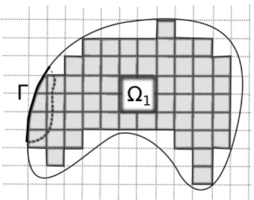
As for every point in Γ there exists a neighborhood whereu=0a.e., then in a neighborhood Ω∗ of Γ we haveu=0a.e.. From this neighborhood, using hyperrectangles as in Figure 1(b) we can extend the equalityu=0a.e.. The set Ω can be covered by a net of hyperrectangles stemming from Ω∗, covering a subset Ω1 (Figure 2). Next, we use smaller hyperrectangles covering a greater

set Ω2⊂Ω and so on, using at most countable many hyperrectangles, obtaining

u=0a.e. in Ω. X

(a) Area of integration. (b) Extension by rectangles. Figure 1

The system of equations related toB is

−X

i,j

∂l

dijkl

eij+

X

s

cs_ijus

+X i,j

qijk

eij+

X

s

cs_ijus

Γ

Figure 2.The functionuis zero in the region Ω1, depicted by gray rectangles.

where dijkl_=aijkl_+aijlk_{, q}ijk ₌P

s,ta ijst_ck

st andeij =∂iuj+∂jui. Natural conditions are

X

i,j,l

dijkl

eij+

X

s

cs_ijus

nl=gk. (22)

So we have established the following theorem.

Theorem 3.2. Letf : Ω⊂Rn→Rn andg:∂Ω−Γ→Rn be vector functions

such that

f ∈

Lp(Ω)n

and g∈

Lp∗(∂Ω−Γ)n

for 1< p, p∗≤ ∞, if n= 2,

f ∈hLn2+2n (Ω)

in

and g∈hL2(nn−1)(∂Ω−Γ)

in

, if n >2.

Then for the system of partial differential equations (21)with boundary condi-tions (6)and (22)exists a unique solution inH.

Acknowledgements. This work was supported by Universidad Nacional de Colombia, Bogot´a, under grant No. 17105. The first author was supported by a grant from MAZDA Foundation for Art and Science.

References

[1] G. Acosta, R. G. Dur´an, and F. L. Garc´ıa,Korn Inequality and Divergence Operator: Counterexamples and Optimality of Weighted Estimates, Proc. Amer. Math. Soc.141(2013), 217–232.

[2] R. A. Adams and J. F. Fournier,Sobolev Spaces, 2nd ed., Elsevier, Ams-terdam, The Netherlands, 2003.

[3] H. Altenbach, V. A. Eremeyev, and L. P. Lebedev, On the Existence of Solution in the Linear Elasticity with Surface Stresses, ZAMM90(2010), 231–240.

[4] , On the Spectrum and Stiffness of an Elastic Body with Surface Stresses, ZAMM91(2011), 699–710.

[5] P. G. Ciarlet,Mathematical Elasticity. Vol. I: Three-Dimensional Elastic-ity, vol. 1, Elsevier, Amsterdam, The Netherlands, 1988.

[6] S. Conti, D. Faraco, and F. Maggi,A New Approach to Counterexamples toL1_{Estimates: Korn’s Inequality, Geometric Rigidity, and Regularity for}

Gradients of Separately Convex Functions, Arch. Rational Mech. Anal.

175(2005), 287–300.

[7] H. L. Duan, J. Wang, and B. L. Karihaloo, Theory of Elasticity at the Nanoscale, Advances in Applied Mechanics 42(2009), 1–68.

[8] G. Fichera, Handbuch der Physik, ch. Existence Theorems in Elasticity, Springer, Berlin, Germany, 1972 (de).

[9] K. O. Friederichs,On the Boundary-Value Problems of the Theory of Elas-ticity and Korn’s Inequality, Ann. of Math.48(1947), 441–471.

[10] M. E. Gurtin and A. I. Murdoch,A Continuum Theory of Elastic Material Surfaces, Arch. Rat. Mech. Analysis57(1975), 291–323.

[11] C. O. Horgan, Korn’s Inequalities and Their Applications in Continuum Mechanics, SIAM rev.37(1995), no. 4, 491–511.

[12] V. A. Kondrat’ev and O. A. Oleynik, Boundary-value Problems for the System of Elasticity Theory in Unbounded Domains. Korn’s Inequalities, Russ. Math. Surv.43(1988), no. 5, 65–119.

[13] A. Korn, Solution g´en´erale du probl`eme d’´equilibre dans la th´eorie de l’´elasticit´e dans le cas o`u les efforts sont donn`es `a la surface, Ann. Fac. Sci. Toulouse10(1908), no. 2, 165–269 (fr), in french.

[14] , Uber einige Ungleichungen, welche in der Theorie der elastis-¨ chen und elektrischen Schwingungen eine Rolle spielen, Bull. Int. Cra-covie Akademie Umiejet, Classe des Sci. Math. Nat. (1909), 705–724 (de), in german.

[15] L. P. Lebedev, I. I. Vorovich, and M. J. Cloud, Functional Analysis in Mechanics, 2nd ed., Springer-Verlag, New York, USA, 2013.

[16] S. G. Mikhlin, The Problem of the Minimum of a Quadratic Functional, Governmental publisher, Moscow, Rusia, 1952, in russian.

[17] J. Necas and I. Hlav´acek, Mathematical Theory of Elastic and Elasto-Plastic Bodies: An Introduction, Elsevier, 1981.

[18] I. I. Vorovich, Nonlinear Theory of Shallow Shells, Springer-Verlag, New York, USA, 1999.

(Recibido en mayo de 2013. Aceptado en septiembre de 2013)

Departamento de Matem´aticas Universidad Nacional de Colombia Facultad de Ciencias Carrera 30, calle 45 Bogot´a, Colombia

e-mail: [email protected]

e-mail: [email protected]