Blessing of Dimensionality: High-dimensional Feature and Its Efficient
Compression for Face Verification
Dong Chen
Xudong Cao
Fang Wen
Jian Sun
University of Science and Technology of China
Microsoft Research Asia
[email protected] {xudongca,fangwen,jiansun}@microsoft.com
Abstract
Making a high-dimensional (e.g., 100K-dim) feature for face recognition seems not a good idea because it will bring difficulties on consequent training, computation, and stor-age. This prevents further exploration of the use of a high-dimensional feature.
In this paper, we study the performance of a high-dimensional feature. We first empirically show that high dimensionality is critical to high performance. A 100K-dim feature, based on a single-type Local Binary Pattern (LBP) descriptor, can achieve significant improvements over both its low-dimensional version and the state-of-the-art.
We also make the high-dimensional feature practical. With our proposed sparse projection method, named rotated sparse regression, both computation and model storage can be reduced by over 100 times without sacrificing accuracy quality.
1. Introduction
Modern face verification pipelines mainly consist of two stages: extracting low-level features, and building classifi-cation models. The first stage focuses on constructing in-formative features manually or from data. The second stage usually exploits supervised information to learn a classifica-tion model [10,26,30], discriminative subspace [3,26,36], or mid-level representation [4,24,34,38].
A good low-level feature should be both discrimina-tive for inter-person difference and invariant to intra-person variations such as pose/lighting/expression. Recent suc-cessful features have been either handcrafted (e.g., Gabor [27], LBP [1], and SIFT [29]) or learned from data [8]. In the design of a feature, we often compromise its infor-mativeness (containing as much discriminative information as possible) and compactness (size). We favor a compact feature as it makes the second stage easier and whole stor-age/computation cheaper.
However, we question whether such a trade-off
occur-ring in the first stage is too early, w.r.t the whole pipeline. We first study the performance of the high-dimensional fea-ture as the function of its dimensionality (more precise-ly, amount of discriminative information). To effective-ly construct a high-dimensional, informative feature, we appropriately exploit the advantages of the recent strong alignment [7] and other modern techniques. In short, we densely sample multi-scale descriptors centered at dense facial landmarks and concatenate them. We empirically found thata high-dimensional feature, with sufficient train-ing data, is necessary to obtain state-of-the-art results. For example, based on a single-type of LBP descriptor, our high-dimensional feature with 100K-dim can achieve over 93.18% accuracy1 on challenging Labeled Face in Wiled
(LFW) [23] dataset, significantly higher than its non-high-dimensional version and the established state-of-the-art.
Of course, high-dimensional feature leads to high cost. Even if we use a linear dimension reduction method like Principal Component Analysis (PCA), projecting a fea-ture from 100K-dim to 1K-dim needs 100M of expensive floating-point multiplications. Moreover, storage of the pro-jection matrix in floating-point formate is 400M! Such a high cost is unaffordable in many real scenarios such as mo-bile applications or on embedded devices. Even when using a desktop, deploying such system is undesired.
To make high-dimensional feature really useful, we pro-pose a simple two-step scheme for obtaining asparse lin-ear projection. In the first step, any conventional subspace learning methods can be applied to get the compressed, low-dimensional feature. In the second step, we adopt𝑙1 regres-sion to learn a sparse project matrix which maps the feature from the original high dimension to low dimension. Con-sidering that the commonly used distance metrics (e.g., Eu-clidean and Cosine) are invariant to a rotation transforma-tion, we further introduce an additional freedom of rotation in the mapping. Our method, calledRotated Sparse Regres-sion, can reduce the cost of linear projection and its storage
1Under unrestricted protocol; no outside training data in recognition
system.
by sacrificing very little accuracy (less than 0.1%). The main contributions of this paper are:
∙ We reveal the significance of a high-dimensional fea-ture in the context of modern technology (face align-ment / learning methods / massive data) for face recog-nition;
∙ We propose a rotated sparse regression to make high-dimensional feature feasible;
∙ We demonstrate state-of-the-art performances of the high-dimensional feature, in various settings (unsuper-vised / limited training / unlimited training).
2. Related Works
Since the topics covered in face recognition literature are numerous, we focus on two most-related aspects.
Over-completed representationis an effective way to ob-tain an informative, high-dimensional feature. In unsuper-vised feature learning, densely sampling overlapped image patches [5,12] consistently improve performance. For ex-ample, Coated et al. [12] discovered through experimen-tation that over-completed bases are critical to high perfor-mance regardless of the choice of encoding methods. Simi-lar observations have also been made in [5,22,37].
Multi-scales sampling has also proven be effective. Ex-amples include multi-scale LBP [9] and multi-scale SIFT [18,19] for face recognition, Gist descriptor for image re-trieval [14], and scene classification [32,35].
Feature compression. Two common approaches for com-pressing features are feature selection and the subspace method. Feature selection is the most effective way to re-move noisy and irrelevant dimensions. It is usually formu-lated in a greedy way such as boosting [15], or in a more principled way by enforcing𝑙1penalty [20] or structure s-parsity [28].
The subspace method is more suitable for extracting the most discriminative low-dimensional representation. It can be implemented as an unsupervised [21,36] or supervised subspace methods [3,10,26]. For linear subspace meth-ods, the high-dimensional feature is projected into a low-dimensional subspace with a linear projection. To make the projection sparse, Hastieet al. developed a sparse version of PCA [41] and LDA [11] by adding a sparse penalty and formulating them as elastic net problems [40]. However, the additional sparse penalty often makes the original optimiza-tion method inapplicable. This drawback could become an insurmountable obstacle when trying to enforce sparsity to other more sophisticated subspace learning methods.
3. High-dimensional Feature is Necessary
In this section, we describe our construction of the high-dimensional feature in detail and study its accuracy though
(a)
(b)
Figure 1. (a) shows the fiducial points used in the high-dimensional feature, we found denser fiducial points significantly improve the performance of the feature. (b) explains the multi-scales represen-tation. The small scale describes the detailed appearance around the fiducial points and the large scale captures the shape of face in relative large range.
experimentation as a function of the dimensionality.
3.1. Constructing high-dimensional feature
We construct the feature simply by extracting multi-scale patches centered at dense facial landmarks. We first locate dense facial landmarks with a recent face alignment method [7] and rectify similarity transformation based on five land-marks (eyes, nose, and mouth corners). Then, we extract multi-scale image patches centered around each landmark. We divide each patch into a grid of cells and code each cell by a certain descriptor. Finally, we concatenate all descrip-tors to form our high-dimensional feature.
In the above process, the following two factors are worth noting.
Dense landmarks. Our feature is based on accurate and dense facial landmarks. This is only possible with recent great progress made in face alignment (i.e. locating land-marks) [2,7]. Using sampling or regression techniques, to-day’s face alignment methods can output both accurate and dense landmarks on faces in the wild. In this paper, we leverage these works and show that this factor is crucial to our work.
We select landmarks of the inner face due to their rela-tively high accuracy and reliability. Figure 1 (a) (from s-parse to dense) shows the landmarks we used for feature extraction, which are salient points on the eye brows, eyes, nose and mouth. There are 27 landmarks in total.
Multiple scales. As shown in Figure1(b), we first build an image pyramid of the normalized facial image (with a similarity transformation which is determined by five land-marks). Then, at each landmark we crop fixed-size image patches on every pyramid layer. Finally the images patches
103 104 105 106 82
84 86 88 90 92 94
Feature Dimension
Accuracy
LE LBP SIFT HOG Gabor
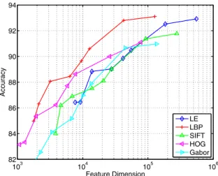
Figure 2. Accuracy as a function of the features dimension.
at all layers are divided into 4x4 cells which are described by a certain kind of local descriptor.
Note that our patch size is very large. For example, the patch at the third layer covers more than half the area of the face. We found this is important because such a large patch contains global shape information.
3.2. High dimensionality leads to high performance
In this section, we investigate the effect of the dimen-sionality of our feature on face verification accuracy. We use the LFW benchmark, following its unrestricted pro-tocol [23]. We evaluate five different local descriptors: LBP [1], SIFT [29], HOG [13], Gabor [27], and LE [8].
Figure1 shows our main result: high-dimensional fea-ture results in high performance. There is a6%∼7% im-provement in accuracy when increasing the dimensionality from 1K to over 100K for all descriptors. In this experimen-t, the feature dimension is increased by varying landmark numbers from 5 to 27 and sampling scales from 1 to 5.
To effectively apply a supervised learning method in the second stage, the dimension of these features is reduced to 400 by PCA2. We compared three leading learning
meth-ods, LDA [3], PLDA [26], and Joint Bayesian [10]. Our results held regardless of the choice of supervised learning methods. For simplicity, we only report the results from the Joint Bayesian method, which consistently achieves best ac-curacy.
We believe the results of the high performance of high-dimensional feature are due to a few reasons. First, the land-marks based sampling make the feature invariant to varia-tions like poses and expressions. Second, dense landmark-s functionlandmark-s landmark-similar to the denlandmark-se landmark-sampling in BOV frame-work [5,12], which includes more information by the over-completed representation. Third, the multi-scale sampling
2The results are similar from 400 to 1,000.
effectively and comprehensively encodes the micro and macro structures of the face. Last, the previous factors are not redundant. They are complementary. We will conduct more detailed experiments to further investigate these fac-tors in Section5.1.
Note that the effectiveness of the high-dimensional fea-ture may be limited by insufficient training data. But nowa-days, larger datasets are gradually available in research [10,23] and industry [33]. Given sufficient supervised data, the high-dimensional feature is more preferable. In Sec-tion5.2, we will present the results of the high-dimensional feature in a large training data setting.
Recent works on other image classification problems al-so revealed the importance of the high-dimensional feature. Yang et al. [37] showed that over-completed representa-tion is more separable, and S´anchezet al. [31] reported on the significance of high-dimensional features in large-scale image classification. Pooling in spatial [25] and feature s-paces [6] also lead to higher dimensionality and better per-formance.
4. Rotated Sparse Regression based Efficient
Compression
Although high dimensionality leads to high perfor-mance, this comes at a high cost. In this section, we propose a novel method for learning a sparse linear projection which maps the high-dimensional feature to a discriminative sub-space with a much lower computational/storage cost.
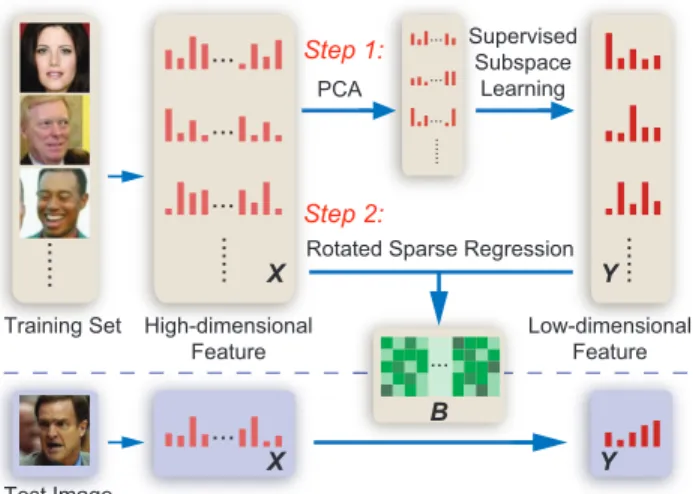
As shown in Figure 3, our method can be divided in-to two steps. In the first step, we adopt PCA to com-press the high-dimensional raw feature. Then the super-vised subspace learning methods such as LDA [3] or Joint Bayesian [10] are applied to extract discriminative informa-tion for face recogniinforma-tion and (potentially) further reduce the dimension.
In the second step, we learn a sparse linear projection which directly maps high-dimensional feature set𝑋to low-dimensional feature set𝑌 learned in the first step. Specifi-cally, we adopt an𝑙1-based regression to learn a sparse ma-trix𝐵with additional freedom in rotation which can further promote the resulting sparsity.
4.1. Rotated sparse regression
Let𝑋 = [𝑥1, 𝑥2, ..., 𝑥𝑁]be the input high-dimensional feature set and 𝑌 = [𝑦1, 𝑦2, ..., 𝑦𝑁]be the corresponding low-dimensional feature set obtained from any conventional subspace learning methods. 𝑁 is the number of training samples. Our objective is to find a sparse linear projection 𝐵which maps𝑋to𝑌 with low error:
min
𝐵 ∥𝑌 −𝐵
𝑇𝑋∥2
...
... ... ...
...
Training Set High-dimensional Feature
... ... ...
...
PCA
Step 1: Supervised Subspace
Learning ed
e
...
Step 2:
X Rotated Sparse Regression Y Low-dimensional
Feature ...
B Test Image
...
X Y
Figure 3. This figure illustrates our method for sparse subspace
learning. In the training phase, low-dimensional features𝑌 are
first obtained by PCA and supervised subspace learning. Then we
learn the sparse projection matrix𝐵 which maps𝑋 to𝑌 by the
rotated sparse regression. In the testing phase, we compute the low-dimensional feature by directly projecting high-dimensional
feature using sparse matrix𝐵.
where the first term is the reconstruction error and the sec-ond term is enforced sparse penalty. The scalar𝜆balances two terms.
Considering the commonly used distance metrics in the subspace (e.g., Euclidean and Cosine) are invariant to ro-tation transformation, we can introduce additional freedom in rotation to promote sparsity without sacrificing accuracy. With an additional rotation matrix𝑅, our new formulation is:
min
𝐵,𝑅 ∥𝑅
𝑇𝑌 −𝐵𝑇𝑋∥2
2+𝜆∥𝐵∥1,
𝑠.𝑡. 𝑅𝑇𝑅=𝐼. (2)
Since the above formulation is a linear regression with s-parse penalty and additional freedom in rotation, we term it asRotated Sparse Regression.
4.2. Optimization
We notice that the objective function is convex if 𝑅or 𝐵 is given. Thus, we adopt an alternative optimization method. The iteration is initialized by simply letting the matrix𝑅be equal to the identity matrix.
Solving B given R.Let𝑌˜ =𝑅𝑇𝑌, the objective function can be rewritten as,
min
𝐵 ∥𝑌˜ −𝐵
𝑇𝑋∥2
2+𝜆∥𝐵∥1. (3) As 𝐵’s columns are independent of each other in E-quation (3), we can optimize each column in parallel. In our implementation, we use an efficient coordinate descent
method [16] which is initialized by the valued obtained in a previous iteration to solve it.
Solving R given B. When matrix 𝐵 is fixed, the sparse penalty term is constant. By removing the constant penalty term from the objective function, we have
min
𝑅 ∥𝑅
𝑇𝑌 −𝐵𝑇𝑋∥2
2,
𝑠.𝑡. 𝑅𝑇𝑅=𝐼. (4)
This problem has a closed form solution. Suppose the SVD decomposition of𝑌 𝑋𝑇𝐵is𝑈𝐷𝑉𝑇, then the closed form solution of matrix𝑅is
𝑅=𝑈𝑉𝑇.
By iteratively optimizing two sub-problems, we can effi-ciently learn a rotated sparse regression.
With the learned linear projection matrix 𝐵, the low-dimensional feature is simply computed by𝐵𝑇𝑋. Due to the sparse penalty, the number of non-zero elements of ma-trix𝐵 is reduced by orders of magnitude (see our experi-ments in Section5.4). As the complexities of linear projec-tion in computaprojec-tion and memory are linear to the number of non-zero elements, the cost of the linear projection is dra-matically reduced.
4.3. Discussion
An alternative approach to sparse subspace learning is directly adding an𝑙1penalty term into the original objective function [41,11]. Despite such an approach being more ele-gant in the formulation, they cause difficulties for optimiza-tion. In contrast, our method directly exploits the original subspace method to compute the low-dimensional feature and avoid difficulties in developing new optimization meth-ods. Moreover, since only the low-dimensional feature is required in the second step, it is not necessary for the orig-inal subspace learning method to be linear. In addition, the rotation term in our formulation provides additional free-dom and further promotes the sparsity.
Feature selection is also a common approach to dealing with high-dimension problems such as boosting [15] and multi-task feature selection [28]. It aims to select a subset of dimensions which contains more discriminative informa-tion and remove the noise and redundancy. Compared with feature selection methods, our method exploits the infor-mation in all dimensions rather than a subset of them. As shown in Section5.5, our method achieves much better per-formance, which indicates most of dimensions are useful in our constructed high-dimensional feature.
5. Experimental Results
In this section, we present more experimental results of our high-dimensional feature and rotated sparse
regres-sion method. We evaluate the high-dimenregres-sional feature un-der three settings: unsupervised learning, supervised learn-ing with limited and unlimited trainlearn-ing data. We adop-t adop-the Joinadop-t Bayesian meadop-thod[10]3 for supervised subspace
learning. Before diving into details, we first introduce the three datasets in our experiments and the baseline feature we compare with.
LFW [23]. The LFW database contains 13,233 images from 5,749 identities. The number of images varies from 1 to 530 for one subject. All these images are collected from the Internet with large intra-personal variations. WDRef [10]. The WDRef database contains 99,773 im-ages of 2,995 subjects. Over 2,000 subjects have more than 15 images. They are collected from the Internet with large variations in pose, expression and lighting.
Multi-PIE [17]. The Multi-PIE database contains images of 337 subjects. These images are captured under controlled pose, expression and light conditions.
Baseline feature. The baseline method first normalize the image to 100*100 pixels by an affine transformation calcu-lated based on 5 landmarks (two eyes, noise and two mouth tips). Then, the image is divided into 10*10 no-overlapped cells. Each cells within the image is mapped to a vector by a certain descriptor. All descriptors are concatenated to form the final feature.
5.1. The High-dimensional feature is better
In the first experiment, we evaluate the performance of the high-dimensional feature with supervised learning. We extract image patches at 27 landmarks in 5 scales4. The
patch size is fixed to40×40in all scales. We divide each patch into4×4non-overlapped cells. We evaluate 5 de-scriptors for encoding each cell: LE [8], LBP [1], SIFT [29], HOG [13] and Gabor [27]. The dimension of the features are reduced to 400 by PCA for supervised learning. We fol-low LFW’s “unrestricted protocol” - only use training data provided by LFW.
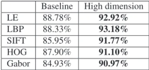
As shown in Table 1, compared with the baseline fea-ture, the high-dimensional feature brings 4% ∼ 6% gain in accuracy for all descriptors. The single LBP descriptor obtains93.18%which is2%higher than the state-of-the-art result [10] which is based on multiple feature combination. To better understand our high-dimensional feature, we separately investigate three factors: sampling at landmarks, landmark number, and scale number.
Sampling at landmarks.To investigate this factor, we ex-tract image patches in a single scale at 9 landmarks and compare it with the baseline feature. Their dimensionality
3We have tried several supervised learning methods such as LDA [3],
PLDA [26] and Joint Bayesian [10]. According to our experiments, the accuracy consistently improved. Given limited space, we only report the results of Joint Bayesian which achieved the best results.
4The normalized facial image are resized to five scales. The side
length-s of the image in each length-scale are 300, 212, 150, 106, 75.
Baseline High dimension
LE 88.78% 92.92%
LBP 88.33% 93.18%
SIFT 85.95% 91.77%
HOG 87.90% 91.10%
Gabor 84.93% 90.97%
Table 1. The comparison between the high-dimensional feature and the baseline feature under LFW unrestricted protocol.
Baseline Sampling at landmarks
LE 88.78% 90.60%
LBP 88.33% 90.30%
SIFT 85.95% 89.08%
HOG 87.90% 88.78%
Gabor 84.93% 87.27%
Table 2. The comparison between sampling at regular grids (Base-line) and sampling at landmarks.
are kept close so as to exclude the impact of the dimension-ality. As shown in Table2, sampling at the landmarks leads to comparatively better performance, which indicates sam-pling at the landmarks effectively reduce the intra-personal geometric variations due to pose and expressions.
Landmark number. In this experiment, we increase the landmarks number from 5 to 27 to investigate performance as a function of the number of landmarks. Figure4shows the accuracies of all descriptors improve monotonically, when the number of landmarks increases from 5 to 22. In-creasing from 22 to 25 will not cause much improvement or even bring small negative effect.
Scale number.To verify the effect of multi-scale represen-tation, we conduct experiments to study the performance with varying numbers of scales. We can see from Fig-ure5that the accuracy of all descriptors increases when the number of scales increases. The accuracy gain is around 2%∼3%, when we raise the number of scales from 1 to 5. But after 5 scales, the benefit becomes marginal.
5.2. Large scale dataset favors high dimensionality
To investigate the performance of the high-dimensional feature on a large scale dataset, we use the recent Wide and Deep Reference (WDRef) [10] database for training. Since we have more training data now, the feature dimension is reduced to 2,000 by PCA for supervised learning.
As shown in Table3, compared with a smaller training set in LFW, the large-scale dataset leads to an even larger improvement for the high-dimensional feature. Taking the LBP descriptor as an example, the improvement due to high dimensionality is 4.5% on the LFW dataset; On the large s-cale WDRef dataset, the improvement increases to 5.7%. Therefore high dimensionality plays an even more impor-tant role when the size of the training set becomes larger.
5 9 16 22 27 0.81
0.82 0.83 0.84 0.85 0.86 0.87 0.88 0.89 0.9 0.91
Landmark Number
Accuracy
LE LBP SIFT HOG Gabor
Figure 4. The effect of landmark number on performance.
Baseline High dimension
LE 90.28% 94.89%
LBP 89.39% 95.17%
SIFT 86.85% 93.21%
HOG 88.93% 93.40%
Gabor 87.38% 92.83%
Table 3. The comparison between the high-dimensional feature and the baseline feature. Training is on WDRef and testing is on LFW.
5.3. High-dimensional feature with unsupervised
learning
In this experiment, we study the impact of high dimen-sionality under the unsupervised setting. The experiment is carried out on LFW and Multi-PIE databases. For LFW database, we follow LFW’s restricted protocol (no use of identity information). For Multi-PIE databases, we follow the settings in [38] which are similar to LFW protocol. We first reduce the dimension of the feature to 400 by PCA and then compute the cosine similarity of a pair of faces.
As shown in the Table 4, in both databases, the high-dimensional features are3%∼4%higher than the baseline method, which proves the effectiveness of high dimension-ality in the unsupervised setting.
5.4. Compression by rotated sparse regression
In this experiment, we evaluate the proposed rotated s-parse regression method by comparing it with a ss-parse re-gression based on Equation1. By varying the value of𝜆, we compare the sparse regression and the rotated sparse regres-sion under different sparsity. We follow the LFW unrestrict-ed protocol and report the average sparsity (the proportion of zeros elements) over 10 rounds.
1 2 3 4 5
0.84 0.85 0.86 0.87 0.88 0.89 0.9 0.91
Scale Number
Accuracy
LE LBP SIFT HOG Gabor
Figure 5. This figure shows the effect of multi-scale representation.
LFW Multi-PIE
Baseline High dim Baseline High dim LE 81.05% 84.58% 83.27% 87.23% LBP 80.05% 84.08% 80.60% 83.92% SIFT 77.17% 83.03% 79.30% 83.97% HOG 80.08% 84.98% 82.98% 87.08% Gabor 74.97% 82.02% 81.05% 85.12%
Table 4. The comparison between the high-dimensional feature and the baseline feature on LFW and Multi-PIE database under unsupervised setting.
Sparsity Compression Sparse Rotated Sparse Ratio Regression Regression
0.95 20 93.18% 93.18%
0.98 50 92.93% 93.18%
0.99 100 92.05% 93.09%
0.995 200 91.43% 92.98%
Table 5. The comparison of the sparse regression and rotated s-parse regression under various sparsity.
Without the sparse penalty, the high-dimensional LBP achieves 93.18% under the LFW unrestricted protocol. As shown in Table5, both methods maintain accuracy when the sparsity is 0.95. However, when the sparsity goes beyond 0.98, the proposed rotated sparse regression can still retain fairly good accuracy, but sparse regression suffers from a significant accuracy drop. This is due to the additional ro-tation freedom. It makes the projection matrix more sparse given the same reconstruction error. When sparsity increas-es to 0.99, with the aid of rotated sparse regrincreas-ession, we re-duce the cost of linear projection by 100 times with less than 0.1% accuracy drop.
0.2 0.3 0.4 0.5 0.6 0.7 0.8 0.9 1 0.86
0.87 0.88 0.89 0.9 0.91 0.92 0.93 0.94
Sparsity
Accuracy
No Sparse Compression Backward Greedy Structure Sparsity Rotated Sparse Regression
Figure 6. This figure compares the rotated sparse regression and two feature selection methods
5.5. Comparison with Feature Selection
In this experiment, we compare the rotated sparse re-gression and two feature selection methods: backward greedy [39] and structure sparsity [28]. We use the high-dimensional LBP feature as input in all methods. For back-ward greedy, we treat each image patch as a selection unit. In each iteration, we remove the image patch that leads to the smallest drop in accuracy. For structure sparsity, we follow the method in [28] which uses𝑙2,1-norm to enforce structure sparsity for feature selection.
As shown in Figure6, feature selection methods suffer from a significant accuracy drop when sparsity is larger than 60%. When sparsity is around 80%, the rotated sparse re-gression is slightly better than no sparse compression, as s-parsity may promote generalization. When ss-parsity is high-er than90%, our method outperforms the feature selection method by6%, which verifies the effectiveness of the pro-posed method. It also indicates that the majority of dimen-sions in our high-dimensional feature are informative and complementary. Simply removing a subset of them will lose information and lead to a performance drop.
5.6. Comparison with the state-of-the-art
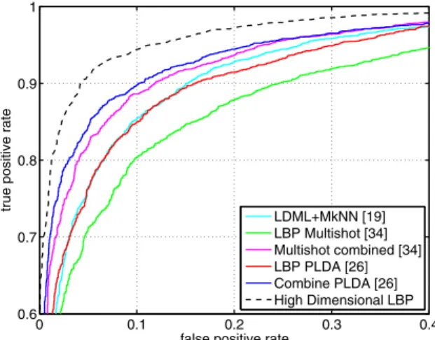
Finally, we make a comparison with the state-of-the-art methods under two settings: supervised learning without and with outside training data. We achieve93.18%(2nd best is 90.07% [26]) under the LFW unrestricted protocol (know identity information). Using WDRef as outside train-ing data, we achieve95.17%(2nd best is 93.30% [4]). As shown in Figures7and8, our method significantly outper-forms the state-of-the-art method under both settings.
6. Conclusion
In this paper, we have studied the performance of face feature as a function of dimensionality. We have shown
0 0.1 0.2 0.3 0.4
0.6 0.7 0.8 0.9 1
false positive rate
true positive rate
LDML+MkNN [19] LBP Multishot [34] Multishot combined [34] LBP PLDA [26] Combine PLDA [26] High Dimensional LBP
Figure 7. The ROC curve. The training set is LFW.
0 0.1 0.2 0.3 0.4
0.6 0.7 0.8 0.9 1
false positive rate
true positive rate
Attribute and simile classifiers [24] Associate−Predict [38]
face.com r2011b [33] CMD+SLBP [22] Tom−vs−Pete [4] High Dimensional LBP
Figure 8. The ROC curve. The training set is WDRef.
through experimentation that high dimensionality is criti-cal to achieving high performance. We also made the high-dimensional feature practical enough to be introduced into a rotated sparse regression technique. We hope our promising results can encourage more work on building more informa-tive features and increased studying of better compression solutions.
References
[1] T. Ahonen, A. Hadid, and M. Pietikainen. Face Description with Local Binary Patterns: Application to Face
Recogni-tion.IEEE Trans on PAMI, 28:2037–2041, 2006. 1,3,5
[2] P. Belhumeur, D. Jacobs, D. Kriegman, and N. Kumar. Lo-calizing parts of faces using a consensus of exemplars. In
CVPR, pages 545–552. IEEE, 2011.2
[3] P. N. Belhumeur, J. P. Hespanha, and D. J. Kriegman. Eigen-faces vs. FisherEigen-faces: Recognition Using Class Specific
Lin-ear Projection.IEEE Trans on PAMI, 1997.1,2,3,5
[4] T. Berg and P. N. Belhumeur. Tom-vs-Pete Classifiers and
Identity-Preserving Alignment for Face Verification. In
[5] Y. Boureau, F. Bach, Y. LeCun, and J. Ponce. Learning
mid-level features for recognition. InComputer Vision and
Pat-tern Recognition, pages 2559–2566. IEEE, 2010.2,3 [6] Y. Boureau, N. Le Roux, F. Bach, J. Ponce, and Y. LeCun.
Ask the locals: multi-way local pooling for image
recogni-tion. InICCV, pages 2651–2658, 2011.3
[7] X. Cao, Y. Wei, F. Wen, and J. Sun. Face alignment by
explicit shape regression. InComputer Vision and Pattern
Recognition, pages 2887 –2894, June 2012.1,2
[8] Z. Cao, Q. Yin, X. Tang, and J. Sun. Face recognition with
learning-based descriptor. InComputer Vision and Pattern
Recognition, pages 2707–2714, 2010.1,3,5
[9] C. Chan, J. Kittler, and K. Messer. Multi-scale local binary
pattern histograms for face recognition.Advances in
biomet-rics, pages 809–818, 2007.2
[10] D. Chen, X. Cao, L. Wang, F. Wen, and J. Sun. Bayesian
face revisited: A joint formulation. InEuropean Conference
on Computer Vision, pages 566–579, 2012.1,2,3,5 [11] L. Clemmensen, T. Hastie, D. Witten, and B. Ersboll. Sparse
discriminant analysis.Technometrics, 2011.2,4
[12] A. Coates, H. Lee, and A. Ng. An analysis of
single-layer networks in unsupervised feature learning.Ann Arbor,
1001:48109, 2010.2,3
[13] N. Dalal and B. Triggs. Histograms of Oriented Gradients for
Human Detection. InComputer Vision and Pattern
Recogni-tion, volume 1, pages 886–893, 2005.3,5
[14] M. Douze, H. J´egou, H. Sandhawalia, L. Amsaleg, and C. Schmid. Evaluation of gist descriptors for web-scale
im-age search. InInternational Conference on Image and Video
Retrieval, page 19, 2009.2
[15] J. Friedman. Greedy function approximation: a gradient
boosting machine.Ann. Statist, 2001.2,4
[16] J. Friedman, T. Hastie, and R. Tibshirani. Regularization Paths for Generalized Linear Models via Coordinate Descen-t.Journal of statistical software, 33(1):1–22, 2010. 4 [17] R. Gross, I. Matthews, J. Cohn, T. Kanade, and S. Baker.
Multi-pie. InInternational Conference on Automatic Face
and Gesture Recognition, 2008.5
[18] M. Guillaumin, T. Mensink, J. J. Verbeek, and C. Schmid. Automatic face naming with caption-based supervision. In
CVPR, pages 1–8, 2008.2
[19] M. Guillaumin, J. Verbeek, and C. Schmid. Is that you?
Met-ric learning approaches for face identification. In2009 IEEE
12th International Conference on Computer Vision, pages
498–505. IEEE, Sept. 2009.2
[20] I. Guyon and A. Elisseeff. An introduction to variable and
feature selection. The Journal of Machine Learning
Re-search, 3:1157–1182, 2003.2
[21] X. He, S. Yan, Y. Hu, P. Niyogi, and H. Zhang. Face
recog-nition using laplacianfaces. IEEE Transactioins on Pattern
Analysis and Machine Intelligence, 27(3):328–340, 2005.2 [22] C. Huang, S. Zhu, and K. Yu. Large scale strongly supervised ensemble metric learning, with applications to face
verifica-tion and retrieval. InNEC Technical Report TR115, 2011.
2
[23] G. B. Huang, M. Ramesh, T. Berg, E. Learned-Miller, and A. Hanson. Labeled Faces in the Wild: A Database for
S-tudying Face Recognition in Unconstrained Environments.
2007.1,3,5
[24] N. Kumar, A. C. Berg, P. N. Belhumeur, and S. K. Nayar.
Attribute and simile classifiers for face verification. InICCV,
pages 365–372. IEEE, Sept. 2009.1
[25] S. Lazebnik, C. Schmid, and J. Ponce. Beyond bags of
features: Spatial pyramid matching for recognizing natural
scene categories. InCVPR, pages 2169–2178, 2006.3
[26] P. Li, U. Mohammed, J. Elder, and S. Prince. Probabilistic
Models for Inference about Identity. IEEE Trans on PAMI,
34:144–157, 2012.1,2,3,5,7
[27] C. Liu and H. Wechsler. Gabor feature based classification using the enhanced fisher linear discriminant model for face
recognition.TIP, 11:467–476, 2002.1,3,5
[28] J. Liu, S. Ji, and J. Ye. Multi-task feature learning via
effi-cient l2,1-norm minimization. InConference on Uncertainty
in Artificial Intelligence, pages 339–348, 2009.2,4,7 [29] D. G. Lowe. Distinctive Image Features from Scale-Invariant
Keypoints.IJCV, 60:91–110, 2004.1,3,5
[30] B. Moghaddam, T. Jebara, and A. Pentland. Bayesian face
recognition.Pattern Recognition, 2000.1
[31] J. Sanchez and F. Perronnin. High-dimensional signature
compression for large-scale image classification. InCVPR,
pages 1665–1672, 2011.3
[32] C. Siagian and L. Itti. Rapid biologically-inspired scene
clas-sification using features shared with visual attention.Pattern
Analysis and Machine Intelligence, 29(2):300–312, 2007.2 [33] Y. Taigman and L. Wolf. Leveraging billions of faces to overcome performance barriers in unconstrained face
recog-nition. arXiv:1108.1122, 2011.3
[34] Y. Taigman, L. Wolf, and T. Hassner. Multiple One-Shots for
Utilizing Class Label Information. InBritish Machine Vision
Conference, 2009.1
[35] A. Torralba, K. Murphy, W. Freeman, and M. Rubin. Context-based vision system for place and object
recogni-tion. InInternational Conference on Computer Vision, pages
273–280, 2003.2
[36] M. Turk and A. Pentland. Face recognition using
eigen-faces. InComputer Vision and Pattern Recognition, 1991.
Proceedings CVPR ’91., IEEE Computer Society Conference
on, pages 586 –591, jun 1991.1,2
[37] J. Yang, K. Yu, Y. Gong, and T. Huang. Linear spatial pyra-mid matching using sparse coding for image classification. InComputer Vision and Pattern Recognition, pages 1794–
1801, 2009.2,3
[38] Q. Yin, X. Tang, and J. Sun. An associate-predict model for
face recognition. InComputer Vision and Pattern
Recogni-tion, pages 497–504, 2011.1,6
[39] T. Zhang. Adaptive forward-backward greedy algorithm
for learning sparse representations. Information Theory,
57(7):4689 –4708, july 2011.7
[40] H. Zou and T. Hastie. Regularization and variable selection
via the elastic net. Journal of the Royal Statistical Society:
Series B (Statistical Methodology), 67(2):301–320, 2005.2 [41] H. Zou, T. Hastie, and R. Tibshirani. Sparse Principal
Com-ponent Analysis. Journal of Computational and Graphical