Adaptive Computation and Machine Learning Thomas Dietterich, Editor
Christopher Bishop, David Heckerman, Michael Jordan, and Michael Kearns, Associate Editors
Bioinformatics: The Machine Learning Approach, Pierre Baldi and Søren Brunak
Reinforcement Learning: An Introduction, Richard S. Sutton and Andrew G. Barto
Graphical Models for Machine Learning and Digital Communication, Brendan J. Frey
Learning in Graphical Models, Michael I. Jordan
Causation, Prediction, and Search, second edition, Peter Spirtes, Clark Glymour, and Richard Scheines Principles of Data Mining,
David Hand, Heikki Mannila, and Padhraic Smyth
Bioinformatics: The Machine Learning Approach, second edition, Pierre Baldi and Søren Brunak
Learning Kernel Classifiers: Theory and Algorithms, Ralf Herbrich
Learning with Kernels: Support Vector Machines, Regularization, Optimization, and Beyond, Bernhard Sch¨olkopf and Alexander J. Smola
Introduction to Machine Learning, Ethem Alpaydin
Gaussian Processes for Machine Learning,
Gaussian Processes for Machine Learning
Carl Edward Rasmussen Christopher K. I. Williams
The MIT Press
Cambridge, Massachusetts London, England
c
2006 Massachusetts Institute of Technology
All rights reserved. No part of this book may be reproduced in any form by any electronic or mechanical means (including photocopying, recording, or information storage and retrieval) without permission in writing from the publisher.
MIT Press books may be purchased at special quantity discounts for business or sales promotional use. For information, please emailspecial [email protected] write to Special Sales Department, The MIT Press, 55 Hayward Street, Cambridge, MA 02142.
Typeset by the authors using LATEX 2ε.
This book was printed and bound in the United States of America. Library of Congress Cataloging-in-Publication Data
Rasmussen, Carl Edward.
Gaussian processes for machine learning / Carl Edward Rasmussen, Christopher K. I. Williams. p. cm. —(Adaptive computation and machine learning)
Includes bibliographical references and indexes. ISBN 0-262-18253-X
1. Gaussian processes—Data processing. 2. Machine learning—Mathematical models. I. Williams, Christopher K. I. II. Title. III. Series.
QA274.4.R37 2006 519.2'3—dc22
2005053433
The actual science of logic is conversant at present only with things either certain, impossible, or entirely doubtful, none of which (fortunately) we have to reason on. Therefore the true logic for this world is the calculus of Probabilities, which takes account of the magnitude of the probability which is, or ought to be, in a reasonable man’s mind.
Contents
Series Foreword . . . xi
Preface . . . xiii
Symbols and Notation . . . xvii
1 Introduction 1 1.1 A Pictorial Introduction to Bayesian Modelling . . . 3
1.2 Roadmap . . . 5
2 Regression 7 2.1 Weight-space View . . . 7
2.1.1 The Standard Linear Model . . . 8
2.1.2 Projections of Inputs into Feature Space . . . 11
2.2 Function-space View . . . 13
2.3 Varying the Hyperparameters . . . 19
2.4 Decision Theory for Regression . . . 21
2.5 An Example Application . . . 22
2.6 Smoothing, Weight Functions and Equivalent Kernels . . . 24
∗ 2.7 Incorporating Explicit Basis Functions . . . 27
2.7.1 Marginal Likelihood . . . 29
2.8 History and Related Work . . . 29
2.9 Exercises . . . 30
3 Classification 33 3.1 Classification Problems . . . 34
3.1.1 Decision Theory for Classification . . . 35
3.2 Linear Models for Classification . . . 37
3.3 Gaussian Process Classification . . . 39
3.4 The Laplace Approximation for the Binary GP Classifier . . . 41
3.4.1 Posterior . . . 42
3.4.2 Predictions . . . 44
3.4.3 Implementation . . . 45
3.4.4 Marginal Likelihood . . . 47
∗ 3.5 Multi-class Laplace Approximation . . . 48
3.5.1 Implementation . . . 51
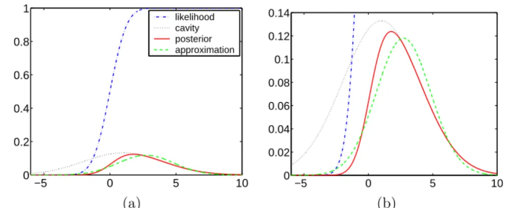
3.6 Expectation Propagation . . . 52
3.6.1 Predictions . . . 56
3.6.2 Marginal Likelihood . . . 57
3.6.3 Implementation . . . 57
3.7 Experiments . . . 60
3.7.1 A Toy Problem . . . 60
3.7.2 One-dimensional Example . . . 62
3.7.3 Binary Handwritten Digit Classification Example . . . 63
3.7.4 10-class Handwritten Digit Classification Example . . . 70
3.8 Discussion . . . 72
viii Contents
∗ 3.9 Appendix: Moment Derivations . . . 74
3.10 Exercises . . . 75
4 Covariance Functions 79 4.1 Preliminaries . . . 79
∗ 4.1.1 Mean Square Continuity and Differentiability . . . 81
4.2 Examples of Covariance Functions . . . 81
4.2.1 Stationary Covariance Functions . . . 82
4.2.2 Dot Product Covariance Functions . . . 89
4.2.3 Other Non-stationary Covariance Functions . . . 90
4.2.4 Making New Kernels from Old . . . 94
4.3 Eigenfunction Analysis of Kernels . . . 96
∗ 4.3.1 An Analytic Example . . . 97
4.3.2 Numerical Approximation of Eigenfunctions . . . 98
4.4 Kernels for Non-vectorial Inputs . . . 99
4.4.1 String Kernels . . . 100
4.4.2 Fisher Kernels . . . 101
4.5 Exercises . . . 102
5 Model Selection and Adaptation of Hyperparameters 105 5.1 The Model Selection Problem . . . 106
5.2 Bayesian Model Selection . . . 108
5.3 Cross-validation . . . 111
5.4 Model Selection for GP Regression . . . 112
5.4.1 Marginal Likelihood . . . 112
5.4.2 Cross-validation . . . 116
5.4.3 Examples and Discussion . . . 118
5.5 Model Selection for GP Classification . . . 124
∗ 5.5.1 Derivatives of the Marginal Likelihood for Laplace’s Approximation 125 ∗ 5.5.2 Derivatives of the Marginal Likelihood for EP . . . 127
5.5.3 Cross-validation . . . 127
5.5.4 Example . . . 128
5.6 Exercises . . . 128
6 Relationships between GPs and Other Models 129 6.1 Reproducing Kernel Hilbert Spaces . . . 129
6.2 Regularization . . . 132
∗ 6.2.1 Regularization Defined by Differential Operators . . . 133
6.2.2 Obtaining the Regularized Solution . . . 135
6.2.3 The Relationship of the Regularization View to Gaussian Process Prediction . . . 135
6.3 Spline Models . . . 136
∗ 6.3.1 A 1-d Gaussian Process Spline Construction . . . 138
∗ 6.4 Support Vector Machines . . . 141
6.4.1 Support Vector Classification . . . 141
6.4.2 Support Vector Regression . . . 145
∗ 6.5 Least-squares Classification . . . 146
Contents ix
∗ 6.6 Relevance Vector Machines . . . 149
6.7 Exercises . . . 150
7 Theoretical Perspectives 151 7.1 The Equivalent Kernel . . . 151
7.1.1 Some Specific Examples of Equivalent Kernels . . . 153
∗ 7.2 Asymptotic Analysis . . . 155
7.2.1 Consistency . . . 155
7.2.2 Equivalence and Orthogonality . . . 157
∗ 7.3 Average-case Learning Curves . . . 159
∗ 7.4 PAC-Bayesian Analysis . . . 161
7.4.1 The PAC Framework . . . 162
7.4.2 PAC-Bayesian Analysis . . . 163
7.4.3 PAC-Bayesian Analysis of GP Classification . . . 164
7.5 Comparison with Other Supervised Learning Methods . . . 165
∗ 7.6 Appendix: Learning Curve for the Ornstein-Uhlenbeck Process . . . 168
7.7 Exercises . . . 169
8 Approximation Methods for Large Datasets 171 8.1 Reduced-rank Approximations of the Gram Matrix . . . 171
8.2 Greedy Approximation . . . 174
8.3 Approximations for GPR with Fixed Hyperparameters . . . 175
8.3.1 Subset of Regressors . . . 175
8.3.2 The Nystr¨om Method . . . 177
8.3.3 Subset of Datapoints . . . 177
8.3.4 Projected Process Approximation . . . 178
8.3.5 Bayesian Committee Machine . . . 180
8.3.6 Iterative Solution of Linear Systems . . . 181
8.3.7 Comparison of Approximate GPR Methods . . . 182
8.4 Approximations for GPC with Fixed Hyperparameters . . . 185
∗ 8.5 Approximating the Marginal Likelihood and its Derivatives . . . 185
∗ 8.6 Appendix: Equivalence of SR and GPR Using the Nystr¨om Approximate Kernel . . . 187
8.7 Exercises . . . 187
9 Further Issues and Conclusions 189 9.1 Multiple Outputs . . . 190
9.2 Noise Models with Dependencies . . . 190
9.3 Non-Gaussian Likelihoods . . . 191
9.4 Derivative Observations . . . 191
9.5 Prediction with Uncertain Inputs . . . 192
9.6 Mixtures of Gaussian Processes . . . 192
9.7 Global Optimization . . . 193
9.8 Evaluation of Integrals . . . 193
9.9 Student’stProcess . . . 194
9.10 Invariances . . . 194
9.11 Latent Variable Models . . . 196
x Contents
Appendix A Mathematical Background 199
A.1 Joint, Marginal and Conditional Probability . . . 199
A.2 Gaussian Identities . . . 200
A.3 Matrix Identities . . . 201
A.3.1 Matrix Derivatives . . . 202
A.3.2 Matrix Norms . . . 202
A.4 Cholesky Decomposition . . . 202
A.5 Entropy and Kullback-Leibler Divergence . . . 203
A.6 Limits . . . 204
A.7 Measure and Integration . . . 204
A.7.1 Lp Spaces . . . 205
A.8 Fourier Transforms . . . 205
A.9 Convexity . . . 206
Appendix B Gaussian Markov Processes 207 B.1 Fourier Analysis . . . 208
B.1.1 Sampling and Periodization . . . 209
B.2 Continuous-time Gaussian Markov Processes . . . 211
B.2.1 Continuous-time GMPs onR . . . 211
B.2.2 The Solution of the Corresponding SDE on the Circle . . . 213
B.3 Discrete-time Gaussian Markov Processes . . . 214
B.3.1 Discrete-time GMPs onZ . . . 214
B.3.2 The Solution of the Corresponding Difference Equation onPN . . 215
B.4 The Relationship Between Discrete-time and Sampled Continuous-time GMPs . . . 217
B.5 Markov Processes in Higher Dimensions . . . 218
Appendix C Datasets and Code 221
Bibliography 223
Author Index 239
Series Foreword
The goal of building systems that can adapt to their environments and learn from their experience has attracted researchers from many fields, including com-puter science, engineering, mathematics, physics, neuroscience, and cognitive science. Out of this research has come a wide variety of learning techniques that have the potential to transform many scientific and industrial fields. Recently, several research communities have converged on a common set of issues sur-rounding supervised, unsupervised, and reinforcement learning problems. The MIT Press series on Adaptive Computation and Machine Learning seeks to unify the many diverse strands of machine learning research and to foster high quality research and innovative applications.
One of the most active directions in machine learning has been the de-velopment of practical Bayesian methods for challenging learning problems. Gaussian Processes for Machine Learning presents one of the most important Bayesian machine learning approaches based on a particularly effective method for placing a prior distribution over the space of functions. Carl Edward Ras-mussen and Chris Williams are two of the pioneers in this area, and their book describes the mathematical foundations and practical application of Gaussian processes in regression and classification tasks. They also show how Gaussian processes can be interpreted as a Bayesian version of the well-known support vector machine methods. Students and researchers who study this book will be able to apply Gaussian process methods in creative ways to solve a wide range of problems in science and engineering.
Preface
Over the last decade there has been an explosion of work in the “kernel ma- kernel machines
chines” area of machine learning. Probably the best known example of this is work on support vector machines, but during this period there has also been much activity concerning the application of Gaussian process models to ma-chine learning tasks. The goal of this book is to provide a systematic and uni-fied treatment of this area. Gaussian processes provide a principled, practical, probabilistic approach to learning in kernel machines. This gives advantages with respect to the interpretation of model predictions and provides a well-founded framework for learning and model selection. Theoretical and practical developments of over the last decade have made Gaussian processes a serious competitor for real supervised learning applications.
Roughly speaking a stochastic process is a generalization of a probability Gaussian process
distribution (which describes a finite-dimensional random variable) to func-tions. By focussing on processes which are Gaussian, it turns out that the computations required for inference and learning become relatively easy. Thus, the supervised learning problems in machine learning which can be thought of as learning a function from examples can be cast directly into the Gaussian process framework.
Our interest in Gaussian process (GP) models in the context of machine Gaussian processes in machine learning
learning was aroused in 1994, while we were both graduate students in Geoff Hinton’s Neural Networks lab at the University of Toronto. This was a time when the field of neural networks was becoming mature and the many con-nections to statistical physics, probabilistic models and statistics became well known, and the first kernel-based learning algorithms were becoming popular. In retrospect it is clear that the time was ripe for the application of Gaussian processes to machine learning problems.
Many researchers were realizing that neural networks were not so easy to neural networks
apply in practice, due to the many decisions which needed to be made: what architecture, what activation functions, what learning rate, etc., and the lack of a principled framework to answer these questions. The probabilistic framework was pursued using approximations byMacKay[1992b] and using Markov chain Monte Carlo (MCMC) methods byNeal[1996]. Neal was also a graduate stu-dent in the same lab, and in his thesis he sought to demonstrate that using the Bayesian formalism, one does not necessarily have problems with “overfitting” when the models get large, and one should pursue the limit of large models. While his own work was focused on sophisticated Markov chain methods for inference in large finite networks, he did point out that some of his networks
became Gaussian processes in the limit of infinite size, and “there may be sim- large neural networks ≡Gaussian processes
pler ways to do inference in this case.”
It is perhaps interesting to mention a slightly wider historical perspective. The main reason why neural networks became popular was that they allowed
the use ofadaptive basis functions, as opposed to the well known linear models. adaptive basis functions
xiv Preface
useful for the modelling problem at hand. However, this adaptivity came at the cost of a lot of practical problems. Later, with the advancement of the “kernel era”, it was realized that the limitation of fixed basis functions is not a big
many fixed basis
functions restriction if only one has enough of them, i.e. typically infinitely many, and one is careful to control problems of overfitting by using priors or regularization. The resulting models are much easier to handle than the adaptive basis function models, but have similar expressive power.
Thus, one could claim that (as far a machine learning is concerned) the adaptive basis functions were merely a decade-long digression, and we are now back to where we came from. This view is perhaps reasonable if we think of models for solving practical learning problems, althoughMacKay[2003, ch. 45], for example, raises concerns by asking “did we throw out the baby with the bath water?”, as the kernel view does not give us any hidden representations, telling
useful representations
us what the useful features are for solving a particular problem. As we will argue in the book, one answer may be to learn more sophisticated covariance functions, and the “hidden” properties of the problem are to be found here. An important area of future developments for GP models is the use of more expressive covariance functions.
Supervised learning problems have been studied for more than a century
supervised learning
in statistics in statistics, and a large body of well-established theory has been developed. More recently, with the advance of affordable, fast computation, the machine learning community has addressed increasingly large and complex problems.
Much of the basic theory and many algorithms are shared between the
statistics and
machine learning statistics and machine learning community. The primary differences are perhaps the types of the problems attacked, and the goal of learning. At the risk of oversimplification, one could say that in statistics a prime focus is often in
data and models
understanding thedataand relationships in terms ofmodelsgiving approximate summaries such as linear relations or independencies. In contrast, the goals in machine learning are primarily to make predictions as accurately as possible and
algorithms and
predictions to understand the behaviour of learningalgorithms. These differing objectives have led to different developments in the two fields: for example, neural network algorithms have been used extensively as black-box function approximators in machine learning, but to many statisticians they are less than satisfactory, because of the difficulties in interpreting such models.
Gaussian process models in some sense bring together work in the two
com-bridging the gap
munities. As we will see, Gaussian processes are mathematically equivalent to many well known models, including Bayesian linear models, spline models, large neural networks (under suitable conditions), and are closely related to others, such as support vector machines. Under the Gaussian process viewpoint, the models may be easier to handle and interpret than their conventional coun-terparts, such as e.g. neural networks. In the statistics community Gaussian processes have also been discussed many times, although it would probably be excessive to claim that their use is widespread except for certain specific appli-cations such as spatial models in meteorology and geology, and the analysis of computer experiments. A rich theory also exists for Gaussian process models
Preface xv
in the time series analysis literature; some pointers to this literature are given in AppendixB.
The book is primarily intended for graduate students and researchers in intended audience
machine learning at departments of Computer Science, Statistics and Applied Mathematics. As prerequisites we require a good basic grounding in calculus, linear algebra and probability theory as would be obtained by graduates in nu-merate disciplines such as electrical engineering, physics and computer science. For preparation in calculus and linear algebra any good university-level text-book on mathematics for physics or engineering such as Arfken [1985] would be fine. For probability theory some familiarity with multivariate distributions (especially the Gaussian) and conditional probability is required. Some back-ground mathematical material is also provided in AppendixA.
The main focus of the book is to present clearly and concisely an overview focus
of the main ideas of Gaussian processes in a machine learning context. We have also covered a wide range of connections to existing models in the literature, and cover approximate inference for faster practical algorithms. We have pre-sented detailed algorithms for many methods to aid the practitioner. Software implementations are available from the website for the book, see AppendixC. We have also included a small set of exercises in each chapter; we hope these will help in gaining a deeper understanding of the material.
In order limit the size of the volume, we have had to omit some topics, such scope
as, for example, Markov chain Monte Carlo methods for inference. One of the most difficult things to decide when writing a book is what sections not to write. Within sections, we have often chosen to describe one algorithm in particular in depth, and mention related work only in passing. Although this causes the omission of some material, we feel it is the best approach for a monograph, and hope that the reader will gain a general understanding so as to be able to push further into the growing literature of GP models.
The book has a natural split into two parts, with the chapters up to and book organization
including chapter5covering core material, and the remaining sections covering the connections to other methods, fast approximations, and more specialized
properties. Some sections are marked by an asterisk. These sections may be ∗
omitted on a first reading, and are not pre-requisites for later (un-starred) material.
We wish to express our considerable gratitude to the many people with acknowledgements
whom we have interacted during the writing of this book. In particular Moray Allan, David Barber, Peter Bartlett, Miguel Carreira-Perpi˜n´an, Marcus Gal-lagher, Manfred Opper, Anton Schwaighofer, Matthias Seeger, Hanna Wallach, Joe Whittaker, and Andrew Zisserman all read parts of the book and provided valuable feedback. Dilan G¨or¨ur, Malte Kuss, Iain Murray, Joaquin Qui˜ nonero-Candela, Leif Rasmussen and Sam Roweis were especially heroic and provided comments on the whole manuscript. We thank Chris Bishop, Miguel Carreira-Perpi˜n´an, Nando de Freitas, Zoubin Ghahramani, Peter Gr¨unwald, Mike Jor-dan, John Kent, Radford Neal, Joaquin Qui˜nonero-Candela, Ryan Rifkin, Ste-fan Schaal, Anton Schwaighofer, Matthias Seeger, Peter Sollich, Ingo Steinwart,
xvi Preface
Amos Storkey, Volker Tresp, Sethu Vijayakumar, Grace Wahba, Joe Whittaker and Tong Zhang for valuable discussions on specific issues. We also thank Bob Prior and the staff at MIT Press for their support during the writing of the book. We thank the Gatsby Computational Neuroscience Unit (UCL) and Neil Lawrence at the Department of Computer Science, University of Sheffield for hosting our visits and kindly providing space for us to work, and the Depart-ment of Computer Science at the University of Toronto for computer support. Thanks to John and Fiona for their hospitality on numerous occasions. Some of the diagrams in this book have been inspired by similar diagrams appearing in published work, as follows: Figure 3.5, Sch¨olkopf and Smola [2002]; Fig-ure5.2,MacKay [1992b]. CER gratefully acknowledges financial support from the German Research Foundation (DFG). CKIW thanks the School of Infor-matics, University of Edinburgh for granting him sabbatical leave for the period October 2003-March 2004.
Finally, we reserve our deepest appreciation for our wives Agnes and Bar-bara, and children Ezra, Kate, Miro and Ruth for their patience and under-standing while the book was being written.
Despite our best efforts it is inevitable that some errors will make it through
errata
to the printed version of the book. Errata will be made available via the book’s website at
http://www.GaussianProcess.org/gpml
We have found the joint writing of this book an excellent experience. Although hard at times, we are confident that the end result is much better than either one of us could have written alone.
Now, ten years after their first introduction into the machine learning
com-looking ahead
munity, Gaussian processes are receiving growing attention. Although GPs have been known for a long time in the statistics and geostatistics fields, and their use can perhaps be traced back as far as the end of the 19th century, their application to real problems is still in its early phases. This contrasts somewhat the application of the non-probabilistic analogue of the GP, the support vec-tor machine, which was taken up more quickly by practitioners. Perhaps this has to do with the probabilistic mind-set needed to understand GPs, which is not so generally appreciated. Perhaps it is due to the need for computational short-cuts to implement inference for large datasets. Or it could be due to the lack of a self-contained introduction to this exciting field—with this volume, we hope to contribute to the momentum gained by Gaussian processes in machine learning.
Carl Edward Rasmussen and Chris Williams T¨ubingen and Edinburgh, summer 2005 Second printing: We thank Baback Moghaddam, Mikhail Parakhin, Leif Ras-mussen, Benjamin Sobotta, Kevin S. Van Horn and Aki Vehtari for reporting errors in the first printing which have now been corrected.
Symbols and Notation
Matrices are capitalized and vectors are in bold type. We do not generally distinguish between proba-bilities and probability densities. A subscript asterisk, such as in X∗, indicates reference to atest set
quantity. A superscript asterisk denotes complex conjugate.
Symbol Meaning
\ left matrix divide: A\bis the vectorxwhich solvesAx=b
, an equality which acts as a definition
c
= equality up to an additive constant
|K| determinant ofK matrix
|y| Euclidean length of vectory, i.e. P
iyi2
1/2
hf, giH RKHS inner product
kfkH RKHS norm
y> the transpose of vectory
∝ proportional to; e.g.p(x|y)∝f(x, y) means thatp(x|y) is equal tof(x, y) times a factor which is independent ofx
∼ distributed according to; example: x∼ N(µ, σ2) ∇or ∇f partial derivatives (w.r.t.f)
∇∇ the (Hessian) matrix of second derivatives 0or0n vector of all 0’s (of lengthn)
1or1n vector of all 1’s (of lengthn)
C number of classes in a classification problem
cholesky(A) Cholesky decomposition: Lis a lower triangular matrix such thatLL>=A cov(f∗) Gaussian process posterior covariance
D dimension of input spaceX
D data set: D={(xi, yi)|i= 1, . . . , n}
diag(w) (vector argument) a diagonal matrix containing the elements of vectorw diag(W) (matrix argument) a vector containing the diagonal elements of matrixW δpq Kronecker delta,δpq= 1 iffp=qand 0 otherwise
EorEq(x)[z(x)] expectation; expectation ofz(x) whenx∼q(x)
f(x) orf Gaussian process (or vector of) latent function values,f = (f(x1), . . . , f(xn))>
f∗ Gaussian process (posterior) prediction (random variable)
¯
f∗ Gaussian process posterior mean
GP Gaussian process: f ∼ GP m(x), k(x,x0)
, the function f is distributed as a Gaussian process with mean functionm(x) and covariance functionk(x,x0) h(x) or h(x) either fixed basis function (or set of basis functions)or weight function H orH(X) set of basis functions evaluated at all training points
I orIn the identity matrix (of sizen)
Jν(z) Bessel function of the first kind
k(x,x0) covariance (or kernel) function evaluated atxandx0 K orK(X, X) n×ncovariance (or Gram) matrix
K∗ n×n∗ matrixK(X, X∗), the covariance between training and test cases
k(x∗) ork∗ vector, short forK(X,x∗), when there is only a single test case
xviii Symbols and Notation
Symbol Meaning
Ky covariance matrix for the (noisy)yvalues; for independent homoscedastic noise,
Ky=Kf +σn2I
Kν(z) modified Bessel function
L(a, b) loss function, the loss of predictingb, whenais true; note argument order log(z) natural logarithm (basee)
log2(z) logarithm to the base 2
`or `d characteristic length-scale (for input dimensiond)
λ(z) logistic function,λ(z) = 1/ 1 + exp(−z) m(x) the mean function of a Gaussian process
µ a measure (see sectionA.7)
N(µ,Σ) orN(x|µ,Σ) (the variablexhas a) Gaussian (Normal) distribution with mean vectorµand covariance matrix Σ
N(x) short for unit Gaussianx∼ N(0, I) nandn∗ number of training (and test) cases
N dimension of feature space
NH number of hidden units in a neural network
N the natural numbers, the positive integers
O(·) big Oh; for functions f and g on N, we write f(n) = O(g(n)) if the ratio f(n)/g(n) remains bounded asn→ ∞
O either matrix of all zerosor differential operator
y|xandp(y|x) conditional random variabley givenxand its probability (density)
PN the regularn-polygon
φ(xi) or Φ(X) feature map of inputxi (or input set X)
Φ(z) cumulative unit Gaussian: Φ(z) = (2π)−1/2Rz
−∞exp(−t
2/2)dt
π(x) the sigmoid of the latent value: π(x) =σ(f(x)) (stochastic iff(x) is stochastic) ˆ
π(x∗) MAP prediction: π evaluated at ¯f(x∗).
¯
π(x∗) mean prediction: expected value ofπ(x∗). Note, in general that ˆπ(x∗)6= ¯π(x∗)
R the real numbers
RL(f) orRL(c) the risk or expected loss forf, or classifierc(averaged w.r.t. inputs and outputs)
˜
RL(l|x∗) expected loss for predictingl, averaged w.r.t. the model’s pred. distr. atx∗
Rc decision region for classc
S(s) power spectrum
σ(z) any sigmoid function, e.g. logisticλ(z), cumulative Gaussian Φ(z), etc. σ2
f variance of the (noise free) signal
σ2
n noise variance
θ vector of hyperparameters (parameters of the covariance function)
tr(A) trace of (square) matrixA
Tl the circle with circumferencel
VorVq(x)[z(x)] variance; variance ofz(x) whenx∼q(x)
X input space and also the index set for the stochastic process X D×nmatrix of the training inputs{xi}ni=1: the design matrix
X∗ matrix of test inputs
xi theith training input
xdi thedth coordinate of theith training inputxi
Chapter 1
Introduction
In this book we will be concerned with supervised learning, which is the problem of learning input-output mappings from empirical data (the training dataset). Depending on the characteristics of the output, this problem is known as either regression, for continuous outputs, or classification, when outputs are discrete.
A well known example is the classification of images of handwritten digits. digit classification
The training set consists of small digitized images, together with a classification from 0, . . . ,9, normally provided by a human. The goal is to learn a mapping from image to classification label, which can then be used on new, unseen images. Supervised learning is an attractive way to attempt to tackle this problem, since it is not easy to specify accurately the characteristics of, say, the handwritten digit 4.
An example of a regression problem can be found in robotics, where we wish robotic control
to learn the inverse dynamics of a robot arm. Here the task is to map from the state of the arm (given by the positions, velocities and accelerations of the joints) to the corresponding torques on the joints. Such a model can then be used to compute the torques needed to move the arm along a given trajectory. Another example would be in a chemical plant, where we might wish to predict the yield as a function of process parameters such as temperature, pressure, amount of catalyst etc.
In general we denote the input as x, and the output (or target) asy. The the dataset
input is usually represented as a vector x as there are in general many input variables—in the handwritten digit recognition example one may have a 256-dimensional input obtained from a raster scan of a 16×16 image, and in the robot arm example there are three input measurements for each joint in the arm. The target y may either be continuous (as in the regression case) or discrete (as in the classification case). We have a datasetDofn observations, D={(xi, yi)|i= 1, . . . , n}.
Given this training data we wish to make predictions for new inputs x∗ training is inductive
that we have not seen in the training set. Thus it is clear that the problem at hand is inductive; we need to move from the finite training data D to a
2 Introduction
functionf that makes predictions for all possible input values. To do this we must make assumptions about the characteristics of the underlying function, as otherwise any function which is consistent with the training data would be equally valid. A wide variety of methods have been proposed to deal with the supervised learning problem; here we describe two common approaches. The
two approaches
first is to restrict the class of functions that we consider, for example by only considering linear functions of the input. The second approach is (speaking rather loosely) to give a prior probability to every possible function, where higher probabilities are given to functions that we consider to be more likely, for example because they are smoother than other functions.1 The first approach
has an obvious problem in that we have to decide upon the richness of the class of functions considered; if we are using a model based on a certain class of functions (e.g. linear functions) and the target function is not well modelled by this class, then the predictions will be poor. One may be tempted to increase the flexibility of the class of functions, but this runs into the danger of overfitting, where we can obtain a good fit to the training data, but perform badly when making test predictions.
The second approach appears to have a serious problem, in that surely there are an uncountably infinite set of possible functions, and how are we going to compute with this set in finite time? This is where the Gaussian
Gaussian process
process comes to our rescue. A Gaussian process is a generalization of the Gaussian probabilitydistribution. Whereas a probability distribution describes random variables which are scalars or vectors (for multivariate distributions), a stochasticprocess governs the properties of functions. Leaving mathematical sophistication aside, one can loosely think of a function as a very long vector, each entry in the vector specifying the function valuef(x) at a particular input x. It turns out, that although this idea is a little na¨ıve, it is surprisingly close what we need. Indeed, the question of how we deal computationally with these infinite dimensional objects has the most pleasant resolution imaginable: if you ask only for the properties of the function at a finite number of points, then inference in the Gaussian process will give you the same answer if you ignore the infinitely many other points, as if you would have taken them all into account! And these answers are consistent with answers to any other finite queries you
consistency
may have. One of the main attractions of the Gaussian process framework is precisely that it unites a sophisticated and consistent view with computational
tractability
tractability.
It should come as no surprise that these ideas have been around for some time, although they are perhaps not as well known as they might be. Indeed, many models that are commonly employed in both machine learning and statis-tics are in fact special cases of, or restricted kinds of Gaussian processes. In this volume, we aim to give a systematic and unified treatment of the area, showing connections to related models.
1These two approaches may be regarded as imposing arestriction bias and apreference bias respectively; see e.g.Mitchell[1997].
1.1 A Pictorial Introduction to Bayesian Modelling 3
0 0.5 1
−2 −1 0 1 2
input, x
f(x)
0 0.5 1
−2 −1 0 1 2
input, x
f(x)
(a), prior (b), posterior
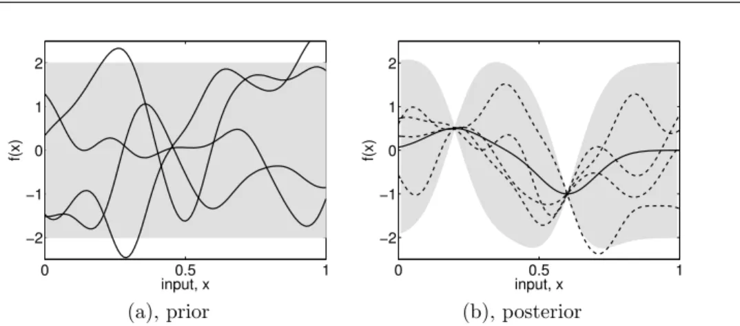
Figure 1.1: Panel (a) shows four samples drawn from the prior distribution. Panel (b) shows the situation after two datapoints have been observed. The mean prediction is shown as the solid line and four samples from the posterior are shown as dashed lines. In both plots the shaded region denotes twice the standard deviation at each input valuex.
1.1
A Pictorial Introduction to Bayesian
Mod-elling
In this section we give graphical illustrations of how the second (Bayesian) method works on some simple regression and classification examples.
We first consider a simple 1-d regression problem, mapping from an input regression
xto an output f(x). In Figure 1.1(a) we show a number of sample functions
drawn at random from theprior distribution over functions specified by a par- random functions
ticular Gaussian process which favours smooth functions. This prior is taken to represent our prior beliefs over the kinds of functions we expect to observe, before seeing any data. In the absence of knowledge to the contrary we have
assumed that the average value over the sample functions at each x is zero. mean function
Although the specific random functions drawn in Figure 1.1(a) do not have a mean of zero, the mean of f(x) values for any fixedxwould become zero, in-dependent of xas we kept on drawing more functions. At any value of xwe
can also characterize the variability of the sample functions by computing the pointwise variance
variance at that point. The shaded region denotes twice the pointwise standard deviation; in this case we used a Gaussian process which specifies that the prior variance does not depend onx.
Suppose that we are then given a dataset D ={(x1, y1),(x2, y2)} consist- functions that agree
with observations
ing of two observations, and we wish now to only consider functions that pass though these two data points exactly. (It is also possible to give higher pref-erence to functions that merely pass “close” to the datapoints.) This situation is illustrated in Figure 1.1(b). The dashed lines show sample functions which are consistent with D, and the solid line depicts the mean value of such func-tions. Notice how the uncertainty is reduced close to the observafunc-tions. The
combination of the prior and the data leads to the posterior distribution over posterior over functions
4 Introduction
If more datapoints were added one would see the mean function adjust itself to pass through these points, and that the posterior uncertainty would reduce close to the observations. Notice, that since the Gaussian process is not a parametric model, we do not have to worry about whether it is possible for the
non-parametric
model to fit the data (as would be the case if e.g. you tried a linear model on strongly non-linear data). Even when a lot of observations have been added, there may still be some flexibility left in the functions. One way to imagine the reduction of flexibility in the distribution of functions as the data arrives is to draw many random functions from the prior, and reject the ones which do not agree with the observations. While this is a perfectly valid way to do inference,
inference
it is impractical for most purposes—the exact analytical computations required to quantify these properties will be detailed in the next chapter.
The specification of the prior is important, because it fixes the properties of
prior specification
the functions considered for inference. Above we briefly touched on the mean and pointwise variance of the functions. However, other characteristics can also be specified and manipulated. Note that the functions in Figure 1.1(a) are smooth and stationary (informally, stationarity means that the functions look similar at all xlocations). These are properties which are induced by the co-variance functionof the Gaussian process; many other covariance functions are
covariance function
possible. Suppose, that for a particular application, we think that the functions in Figure 1.1(a) vary too rapidly (i.e. that their characteristic length-scale is too short). Slower variation is achieved by simply adjusting parameters of the covariance function. The problem oflearning in Gaussian processes is exactly the problem of finding suitable properties for the covariance function. Note, that this gives us a model of the data, and characteristics (such a smoothness,
modelling and
interpreting characteristic length-scale, etc.) which we caninterpret.
We now turn to the classification case, and consider the binary (or
two-classification
class) classification problem. An example of this is classifying objects detected in astronomical sky surveys into stars or galaxies. Our data has the label +1 for stars and−1 for galaxies, and our task will be to predictπ(x), the probability that an example with input vector x is a star, using as inputs some features that describe each object. Obviously π(x) should lie in the interval [0,1]. A Gaussian process prior over functions does not restrict the output to lie in this interval, as can be seen from Figure 1.1(a). The approach that we shall adopt is to squash the prior functionf pointwise through a response function which
squashing function
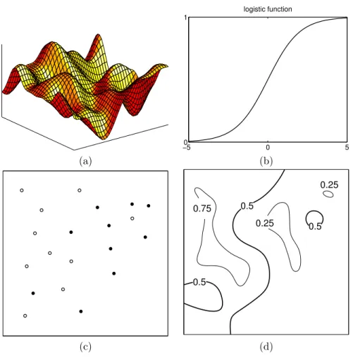
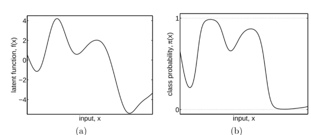
restricts the output to lie in [0,1]. A common choice for this function is the logistic functionλ(z) = (1 + exp(−z))−1, illustrated in Figure1.2(b). Thus the prior overf induces a prior over probabilistic classificationsπ.
This set up is illustrated in Figure 1.2 for a 2-d input space. In panel (a) we see a sample drawn from the prior over functionsf which is squashed through the logistic function (panel (b)). A dataset is shown in panel (c), where the white and black circles denote classes +1 and −1 respectively. As in the regression case the effect of the data is to downweight in the posterior those functions that are incompatible with the data. A contour plot of the posterior mean for π(x) is shown in panel (d). In this example we have chosen a short characteristic length-scale for the process so that it can vary fairly rapidly; in
1.2 Roadmap 5
−50 0 5
1 logistic function
(a) (b)
°
°
°
•
°
°
°
°
°
•
°
• •
• •
• •
°
• •
0.25 0.5
0.5
0.5 0.75
0.25
(c) (d)
Figure 1.2: Panel (a) shows a sample from prior distribution on f in a 2-d input space. Panel (b) is a plot of the logistic functionλ(z). Panel (c) shows the location of the data points, where the open circles denote the class label +1, and closed circles denote the class label −1. Panel (d) shows a contour plot of the mean predictive probability as a function of x; the decision boundaries between the two classes are shown by the thicker lines.
this case notice that all of the training points are correctly classified, including the two “outliers” in the NE and SW corners. By choosing a different length-scale we can change this behaviour, as illustrated in section3.7.1.
1.2
Roadmap
The book has a natural split into two parts, with the chapters up to and includ-ing chapter5 covering core material, and the remaining chapters covering the connections to other methods, fast approximations, and more specialized prop-erties. Some sections are marked by an asterisk. These sections may be omitted on a first reading, and are not pre-requisites for later (un-starred) material.
6 Introduction
Chapter2contains the definition of Gaussian processes, in particular for the
regression
use in regression. It also discusses the computations needed to make predic-tions for regression. Under the assumption of Gaussian observation noise the computations needed to make predictions are tractable and are dominated by the inversion of an×nmatrix. In a short experimental section, the Gaussian process model is applied to a robotics task.
Chapter 3 considers the classification problem for both binary and
multi-classification
class cases. The use of a non-linear response function means that exact compu-tation of the predictions is no longer possible analytically. We discuss a number of approximation schemes, include detailed algorithms for their implementation and discuss some experimental comparisons.
As discussed above, the key factor that controls the properties of a Gaussian
covariance functions
process is the covariance function. Much of the work on machine learning so far, has used a very limited set of covariance functions, possibly limiting the power of the resulting models. In chapter4 we discuss a number of valid covariance functions and their properties and provide some guidelines on how to combine covariance functions into new ones, tailored to specific needs.
Many covariance functions have adjustable parameters, such as the
char-learning
acteristic length-scale and variance illustrated in Figure 1.1. Chapter 5 de-scribes how such parameters can be inferred or learned from the data, based on either Bayesian methods (using the marginal likelihood) or methods of cross-validation. Explicit algorithms are provided for some schemes, and some simple practical examples are demonstrated.
Gaussian process predictors are an example of a class of methods known as
connections
kernel machines; they are distinguished by the probabilistic viewpoint taken. In chapter6we discuss other kernel machines such as support vector machines (SVMs), splines, least-squares classifiers and relevance vector machines (RVMs), and their relationships to Gaussian process prediction.
In chapter 7 we discuss a number of more theoretical issues relating to
theory
Gaussian process methods including asymptotic analysis, average-case learning curves and the PAC-Bayesian framework.
One issue with Gaussian process prediction methods is that their basic
com-fast approximations
plexity isO(n3), due to the inversion of an×nmatrix. For large datasets this is prohibitive (in both time and space) and so a number of approximation methods have been developed, as described in chapter8.
The main focus of the book is on the core supervised learning problems of regression and classification. In chapter9we discuss some rather less standard settings that GPs have been used in, and complete the main part of the book with some conclusions.
AppendixAgives some mathematical background, while AppendixBdeals specifically with Gaussian Markov processes. AppendixCgives details of how to access the data and programs that were used to make the some of the figures and run the experiments described in the book.
Chapter 2
Regression
Supervised learning can be divided into regression and classification problems. Whereas the outputs for classification are discrete class labels, regression is concerned with the prediction of continuous quantities. For example, in a fi-nancial application, one may attempt to predict the price of a commodity as a function of interest rates, currency exchange rates, availability and demand. In this chapter we describe Gaussian process methods for regression problems; classification problems are discussed in chapter3.
There are several ways to interpret Gaussian process (GP) regression models. One can think of a Gaussian process as defining a distribution over functions,
and inference taking place directly in the space of functions, thefunction-space two equivalent views
view. Although this view is appealing it may initially be difficult to grasp, so we start our exposition in section2.1 with the equivalentweight-space view which may be more familiar and accessible to many, and continue in section
2.2with the function-space view. Gaussian processes often have characteristics that can be changed by setting certain parameters and in section2.3we discuss how the properties change as these parameters are varied. The predictions from a GP model take the form of a full predictive distribution; in section2.4
we discuss how to combine a loss function with the predictive distributions using decision theory to make point predictions in an optimal way. A practical comparative example involving the learning of the inverse dynamics of a robot arm is presented in section2.5. We give some theoretical analysis of Gaussian process regression in section2.6, and discuss how to incorporate explicit basis functions into the models in section2.7. As much of the material in this chapter can be considered fairly standard, we postpone most references to the historical overview in section2.8.
2.1
Weight-space View
The simple linear regression model where the output is a linear combination of the inputs has been studied and used extensively. Its main virtues are
simplic-8 Regression
ity of implementation and interpretability. Its main drawback is that it only allows a limited flexibility; if the relationship between input and output can-not reasonably be approximated by a linear function, the model will give poor predictions.
In this section we first discuss the Bayesian treatment of the linear model. We then make a simple enhancement to this class of models by projecting the inputs into a high-dimensional feature space and applying the linear model there. We show that in some feature spaces one can apply the “kernel trick” to carry out computations implicitly in the high dimensional space; this last step leads to computational savings when the dimensionality of the feature space is large compared to the number of data points.
We have a training set D of n observations, D = {(xi, yi) | i= 1, . . . , n},
training set
where x denotes an input vector (covariates) of dimension D and y denotes a scalar output or target (dependent variable); the column vector inputs for all n cases are aggregated in the D ×n design matrix1 X, and the targets
design matrix
are collected in the vector y, so we can write D = (X,y). In the regression setting the targets are real values. We are interested in making inferences about the relationship between inputs and targets, i.e. the conditional distribution of the targets given the inputs (but we are not interested in modelling the input distribution itself).
2.1.1
The Standard Linear Model
We will review the Bayesian analysis of the standard linear regression model with Gaussian noise
f(x) = x>w, y = f(x) +ε, (2.1) wherexis the input vector,wis a vector of weights (parameters) of the linear model,f is the function value andy is the observed target value. Often a bias
bias, offset
weight or offset is included, but as this can be implemented by augmenting the input vectorxwith an additional element whose value is always one, we do not explicitly include it in our notation. We have assumed that the observed values y differ from the function values f(x) by additive noise, and we will further assume that this noise follows an independent, identically distributed Gaussian distribution with zero mean and varianceσ2
n
ε ∼ N(0, σ2n). (2.2)
This noise assumption together with the model directly gives rise to the
likeli-likelihood
hood, the probability density of the observations given the parameters, which is
1In statistics texts the design matrix is usually taken to be the transpose of our definition, but our choice is deliberate and has the advantage that a data point is a standard (column) vector.
2.1 Weight-space View 9
factored over cases in the training set (because of the independence assumption) to give
p(y|X,w) =
n
Y
i=1
p(yi|xi,w) = n
Y
i=1 1 √
2πσn
exp −(yi−x
>
i w)
2
2σ2
n
= 1
(2πσ2
n)n/2
exp − 1 2σ2
n
|y−X>w|2
= N(X>w, σn2I),
(2.3)
where|z|denotes the Euclidean length of vector z. In the Bayesian formalism
we need to specify aprior over the parameters, expressing our beliefs about the prior
parameters before we look at the observations. We put a zero mean Gaussian prior with covariance matrix Σp on the weights
w ∼ N(0, Σp). (2.4)
The rˆole and properties of this prior will be discussed in section 2.2; for now we will continue the derivation with the prior as specified.
Inference in the Bayesian linear model is based on the posterior distribution posterior
over the weights, computed by Bayes’ rule, (see eq. (A.3))2
posterior = likelihood×prior
marginal likelihood, p(w|y, X) =
p(y|X,w)p(w)
p(y|X) , (2.5)
where the normalizing constant, also known as the marginal likelihood (see page marginal likelihood 19), is independent of the weights and given by
p(y|X) = Z
p(y|X,w)p(w)dw. (2.6) The posterior in eq. (2.5) combines the likelihood and the prior, and captures everything we know about the parameters. Writing only the terms from the likelihood and prior which depend on the weights, and “completing the square” we obtain
p(w|X,y) ∝ exp − 1 2σ2
n
(y−X>w)>(y−X>w)
exp −1 2w
>Σ−1
p w
∝ exp −1
2(w−w)¯
> 1
σ2
n
XX>+ Σ−p1(w−w)¯ , (2.7) where ¯w = σn−2(σn−2XX> + Σ−p1)−1Xy, and we recognize the form of the
posterior distribution as Gaussian with mean ¯wand covariance matrixA−1 p(w|X,y) ∼ N( ¯w= 1
σ2
n
A−1Xy, A−1), (2.8) where A = σ−2
n XX>+ Σ−p1. Notice that for this model (and indeed for any
Gaussian posterior) the mean of the posterior distribution p(w|y, X) is also
its mode, which is also called the maximum a posteriori (MAP) estimate of MAP estimate
2Often Bayes’ rule is stated asp(a|b) =p(b|a)p(a)/p(b); here we use it in a form where we additionally condition everywhere on the inputs X (but neglect this extra conditioning for the prior which is independent of the inputs).
10 Regression
intercept, w
1
slope, w
2
−2 −1 0 1 2
−2 −1 0 1 2
−5 0 5
−5 0 5
input, x
output, y
(a) (b)
intercept, w
1
slope, w
2
−2 −1 0 1 2
−2 −1 0 1 2
intercept, w
1
slope, w
2
−2 −1 0 1 2
−2 −1 0 1 2
(c) (d)
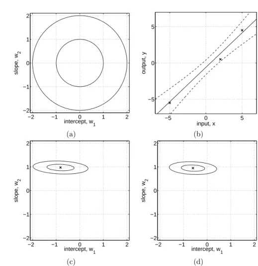
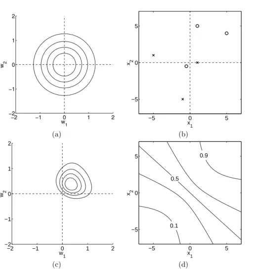
Figure 2.1: Example of Bayesian linear model f(x) = w1 +w2x with intercept
w1 and slope parameter w2. Panel (a) shows the contours of the prior distribution
p(w)∼ N(0, I), eq. (2.4). Panel (b) shows three training points marked by crosses. Panel (c) shows contours of the likelihoodp(y|X,w) eq. (2.3), assuming a noise level of σn= 1; note that the slope is much more “well determined” than the intercept. Panel (d) shows the posterior,p(w|X,y) eq. (2.7); comparing the maximum of the posterior to the likelihood, we see that the intercept has been shrunk towards zero whereas the more ’well determined’ slope is almost unchanged. All contour plots give the 1 and 2 standard deviation equi-probability contours. Superimposed on the data in panel (b) are the predictive mean plus/minus two standard deviations of the (noise-free) predictive distributionp(f∗|x∗, X,y), eq. (2.9).
w. In a non-Bayesian setting the negative log prior is sometimes thought of as a penalty term, and the MAP point is known as the penalized maximum likelihood estimate of the weights, and this may cause some confusion between the two approaches. Note, however, that in the Bayesian setting the MAP estimate plays no special rˆole.3 The penalized maximum likelihood procedure
3In this case, due to symmetries in the model and posterior, it happens that the mean of the predictive distribution is the same as the prediction at the mean of the posterior. However, this is not the case in general.
2.1 Weight-space View 11
is known in this case asridge regression [Hoerl and Kennard, 1970] because of ridge regression
the effect of the quadratic penalty term 12w>Σ−1
p w from the log prior.
To make predictions for a test case we average over all possible parameter predictive distribution
values, weighted by their posterior probability. This is in contrast to non-Bayesian schemes, where a single parameter is typically chosen by some crite-rion. Thus the predictive distribution forf∗,f(x∗) atx∗is given by averaging
the output of all possible linear models w.r.t. the Gaussian posterior p(f∗|x∗, X,y) =
Z
p(f∗|x∗,w)p(w|X,y)dw
= N 1
σ2
n
x>∗A−1Xy, x>∗A−1x∗.
(2.9)
The predictive distribution is again Gaussian, with a mean given by the poste-rior mean of the weights from eq. (2.8) multiplied by the test input, as one would expect from symmetry considerations. The predictive variance is a quadratic form of the test input with the posterior covariance matrix, showing that the predictive uncertainties grow with the magnitude of the test input, as one would expect for a linear model.
An example of Bayesian linear regression is given in Figure 2.1. Here we have chosen a 1-d input space so that the weight-space is two-dimensional and can be easily visualized. Contours of the Gaussian prior are shown in panel (a). The data are depicted as crosses in panel (b). This gives rise to the likelihood shown in panel (c) and the posterior distribution in panel (d). The predictive distribution and its error bars are also marked in panel (b).
2.1.2
Projections of Inputs into Feature Space
In the previous section we reviewed the Bayesian linear model which suffers from limited expressiveness. A very simple idea to overcome this problem is to
first project the inputs into some high dimensional space using a set of basis feature space
functions and then apply the linear model in this space instead of directly on the inputs themselves. For example, a scalar input xcould be projected into
the space of powers of x: φ(x) = (1, x, x2, x3, . . .)> to implement polynomial polynomial regression
regression. As long as the projections are fixed functions (i.e. independent of
the parameters w) the model is still linear in the parameters, and therefore linear in the parameters
analytically tractable.4 This idea is also used in classification, where a dataset
which is not linearly separable in the original data space may become linearly separable in a high dimensional feature space, see section 3.3. Application of this idea begs the question of how to choose the basis functions? As we shall demonstrate (in chapter5), the Gaussian process formalism allows us to answer this question. For now, we assume that the basis functions are given.
Specifically, we introduce the function φ(x) which maps a D-dimensional input vector x into an N dimensional feature space. Further let the matrix
4Models with adaptive basis functions, such as e.g. multilayer perceptrons, may at first seem like a useful extension, but they are much harder to treat, except in the limit of an infinite number of hidden units, see section4.2.3.
12 Regression
Φ(X) be the aggregation of columnsφ(x) for all cases in the training set. Now the model is
f(x) = φ(x)>w, (2.10)
where the vector of parameters now has lengthN. The analysis for this model is analogous to the standard linear model, except that everywhere Φ(X) is substituted forX. Thus the predictive distribution becomes
explicit feature space formulation
f∗|x∗, X,y ∼ N
1 σ2
n
φ(x∗)>A−1Φy, φ(x∗)>A−1φ(x∗)
(2.11) with Φ = Φ(X) and A = σ−2
n ΦΦ>+ Σ−p1. To make predictions using this
equation we need to invert the A matrix of size N ×N which may not be convenient ifN, the dimension of the feature space, is large. However, we can rewrite the equation in the following way
alternative formulation
f∗|x∗, X,y ∼ N φ>∗ΣpΦ(K+σn2I)
−1y,
φ>∗Σpφ∗−φ∗>ΣpΦ(K+σn2I)−
1Φ>Σ
pφ∗
, (2.12) where we have used the shorthand φ(x∗) = φ∗ and defined K = Φ>ΣpΦ.
To show this for the mean, first note that using the definitions of A and K we have σ−n2Φ(K+σ2nI) =σn−2Φ(Φ>ΣpΦ +σn2I) = AΣpΦ. Now multiplying
through by A−1 from left and (K+σn2I)−1 from the right gives σn−2A−1Φ =
ΣpΦ(K+σ2nI)−1, showing the equivalence of the mean expressions in eq. (2.11)
and eq. (2.12). For the variance we use the matrix inversion lemma, eq. (A.9), setting Z−1 = Σ
p, W−1 = σn2I and V = U = Φ therein. In eq. (2.12) we
need to invert matrices of size n×n which is more convenient when n < N.
computational load
Geometrically, note that n datapoints can span at most n dimensions in the feature space.
Notice that in eq. (2.12) the feature space always enters in the form of Φ>ΣpΦ,φ>∗ΣpΦ, orφ>∗Σpφ∗; thus the entries of these matrices are invariably of
the formφ(x)>Σpφ(x0) wherexandx0are in either the training or the test sets.
Let us definek(x,x0) =φ(x)>Σpφ(x0). For reasons that will become clear later
we callk(·,·) acovariance function orkernel. Notice thatφ(x)>Σpφ(x0) is an
kernel
inner product (with respect to Σp). As Σpis positive definite we can define Σ
1/2
p
so that (Σ1p/2)2 = Σp; for example if the SVD (singular value decomposition)
of Σp = U DU>, where D is diagonal, then one form for Σ
1/2
p is U D1/2U>.
Then definingψ(x) = Σ1p/2φ(x) we obtain a simple dot product representation
k(x,x0) =ψ(x)·ψ(x0).
If an algorithm is defined solely in terms of inner products in input space then it can be lifted into feature space by replacing occurrences of those inner products byk(x,x0); this is sometimes called thekernel trick. This technique is
kernel trick
particularly valuable in situations where it is more convenient to compute the kernel than the feature vectors themselves. As we will see in the coming sections, this often leads to considering the kernel as the object of primary interest, and its corresponding feature space as having secondary practical importance.
2.2 Function-space View 13
2.2
Function-space View
An alternative and equivalent way of reaching identical results to the previous section is possible by considering inference directly in function space. We use a Gaussian process (GP) to describe a distribution over functions. Formally:
Definition 2.1 A Gaussian process is a collection of random variables, any Gaussian process
finite number of which have a joint Gaussian distribution.
A Gaussian process is completely specified by its mean function and co- covariance and mean function
variance function. We define mean functionm(x) and the covariance function k(x,x0) of a real processf(x) as
m(x) = E[f(x)],
k(x,x0) = E[(f(x)−m(x))(f(x0)−m(x0))], (2.13) and will write the Gaussian process as
f(x) ∼ GP m(x), k(x,x0). (2.14) Usually, for notational simplicity we will take the mean function to be zero, although this need not be done, see section2.7.
In our case the random variables represent the value of the function f(x) at locationx. Often, Gaussian processes are defined over time, i.e. where the
index set of the random variables is time. This is not (normally) the case in index set≡ input domain
our use of GPs; here the index setX is the set of possible inputs, which could be more general, e.g. RD. For notational convenience we use the (arbitrary)
enumeration of the cases in the training set to identify the random variables such thatfi ,f(xi) is the random variable corresponding to the case (xi, yi)
as would be expected.
A Gaussian process is defined as a collection of random variables. Thus, the definition automatically implies aconsistency requirement, which is also
some-times known as the marginalization property. This property simply means marginalization property
that if the GP e.g. specifies (y1, y2) ∼ N(µ,Σ), then it must also specify y1 ∼ N(µ1,Σ11) where Σ11 is the relevant submatrix of Σ, see eq. (A.6). In other words, examination of a larger set of variables does not change the distribution of the smaller set. Notice that the consistency requirement is au-tomatically fulfilled if the covariance function specifies entries of the covariance
matrix.5 The definition does not exclude Gaussian processes with finite index finite index set
sets (which would be simply Gaussiandistributions), but these are not partic-ularly interesting for our purposes.
5Note, however, that if you instead specified e.g. a function for the entries of theinverse covariance matrix, then the marginalization property would no longer be fulfilled, and one could not think of this as a consistent collection of random variables—this would not qualify as a Gaussian process.
14 Regression
A simple example of a Gaussian process can be obtained from our Bayesian
Bayesian linear model
is a Gaussian process linear regression modelf(x) =φ(x)>w with priorw∼ N(0,Σp). We have for
the mean and covariance
E[f(x)] = φ(x)>E[w] = 0,
E[f(x)f(x0)] = φ(x)>E[ww>]φ(x0) = φ(x)>Σpφ(x0).
(2.15) Thusf(x) andf(x0) are jointly Gaussian with zero mean and covariance given byφ(x)>Σpφ(x0). Indeed, the function valuesf(x1), . . . , f(xn) corresponding
to any number of input pointsnare jointly Gaussian, although ifN < n then this Gaussian is singular (as the joint covariance matrix will be of rankN).
In this chapter our running example of a covariance function will be the squared exponential6 (SE) covariance function; other covariance functions are discussed in chapter4. The covariance function specifies the covariance between pairs of random variables
cov f(xp), f(xq) = k(xp,xq) = exp −12|xp−xq|2. (2.16)
Note, that the covariance between the outputs is written as a function of the inputs. For this particular covariance function, we see that the covariance is almost unity between variables whose corresponding inputs are very close, and decreases as their distance in the input space increases.
It can be shown (see section4.3.1) that the squared exponential covariance function corresponds to a Bayesian linear regression model with an infinite number of basis functions. Indeed for every positive definite covariance function
basis functions
k(·,·), there exists a (possibly infinite) expansion in terms of basis functions (see Mercer’s theorem in section 4.3). We can also obtain the SE covariance function from the linear combination of an infinite number of Gaussian-shaped basis functions, see eq. (4.13) and eq. (4.30).
The specification of the covariance function implies a distribution over func-tions. To see this, we can draw samples from the distribution of functions evalu-ated at any number of points; in detail, we choose a number of input points,7X
∗
and write out the corresponding covariance matrix using eq. (2.16) elementwise. Then we generate a random Gaussian vector with this covariance matrix
f∗ ∼ N 0, K(X∗, X∗), (2.17)
and plot the generated values as a function of the inputs. Figure 2.2(a) shows three such samples. The generation of multivariate Gaussian samples is de-scribed in sectionA.2.
In the example in Figure 2.2 the input values were equidistant, but this need not be the case. Notice that “informally” the functions look smooth.
smoothness
In fact the squared exponential covariance function is infinitely differentiable, leading to the process being infinitely mean-square differentiable (see section
4.1). We also see that the functions seem to have a characteristic length-scale,
characteristic
length-scale 6
Sometimes this covariance function is called the Radial Basis Function (RBF) or Gaussian; here we prefer squared exponential.
7Technically, these input points play the rˆole oftest inputsand therefore carry a subscript asterisk; this will become clearer later when both training and test points are involved.
2.2 Function-space View 15
−5 0 5
−2 −1 0 1 2
input, x
output, f(x)
−5 0 5
−2 −1 0 1 2
input, x
output, f(x)
(a), prior (b), posterior
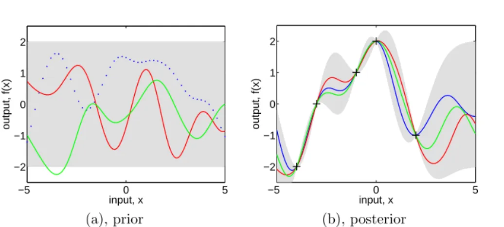
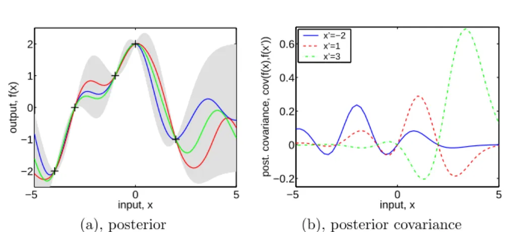
Figure 2.2: Panel (a) shows three functions drawn at random from a GP prior; the dots indicate values ofy actually generated; the two other functions have (less correctly) been drawn as lines by joining a large number of evaluated points. Panel (b) shows three random functions drawn from the posterior, i.e. the prior conditioned on the five noise free observations indicated. In both plots the shaded area represents the pointwise mean plus and minus two times the standard deviation for each input value (corresponding to the 95% confidence region), for the prior and posterior respectively.
which informally can be thought of as roughly the distance you have to move in input space before the function value can change significantly, see section4.2.1. For eq. (2.16) the characteristic length-scale is around one unit. By replacing |xp−xq|by|xp−xq|/`in eq. (2.16) for some positive constant`we could change
the characteristic length-scale of the process. Also, the overall variance of the magnitude
random function can be controlled by a positive pre-factor before the exp in eq. (2.16). We will discuss more about how such factors affect the predictions in section2.3, and say more about how to set such scale parameters in chapter
5.
Prediction with Noise-free Observations
We are usually not primarily interested in drawing random functions from the prior, but want to incorporate the knowledge that the training data provides about the function. Initially, we will consider the simple special case where the
observations are noise free, that is we know{(xi, fi)|i = 1, . . . , n}. The joint joint prior
distribution of the training outputs,f, and the test outputsf∗according to the
prior is
f f∗
∼ N
0,
K(X, X) K(X, X∗)
K(X∗, X) K(X∗, X∗)
. (2.18)
If there are n training points and n∗ test points then K(X, X∗) denotes the
n×n∗ matrix of the covariances evaluated at all pairs of training and test
points, and similarly for the other entriesK(X, X),K(X∗, X∗) andK(X∗, X).
To get the posterior distribution over functions we need to restrict this joint prior distribution to contain only those functions which agree with the observed data points. Graphically in Figure2.2 you may think of generating functions
![Figure 3.5: Panel (a) shows the location of the data points in the two-dimensional space [0, 1] 2](https://thumb-us.123doks.com/thumbv2/123dok_us/8448331.2248968/79.918.120.660.193.742/figure-panel-shows-location-data-points-dimensional-space.webp)
