Improvement of Demand Forecasting Accuracy: A Method Based on Region-Division

Improvement of Demand Forecasting Accuracy:

A Method Based on Region-Division

∗

Guoshan Liu

_{Yuanyuan Lu}

1_{School of Business, Remin University of China, Beijing, P.R.China, 100872} 2_{Mathematical College, Jilin Normal University, Siping, P.R.China, 136000}

Abstract The key factor to increase enterprise profits and reduce the logistic costs is scientific and reasonable logistics demand forecasting, the accuracy of which can directly influence the effect of decision-making for an enterprise. In some instance, a single customer’s demand is irregular, while the demand in a region is comparatively more stable, so it can be better forecasted. In this paper, we have proposed a method to form regions in order that the demand in these regions can be more efficient forecasted while the error of transportation cost caused by replacement of customers by regions can be controlled. Each formed region consists of adjacent customers with similar unit transportation cost to all distributors. Numerical test with data form Northeast Subsidiary Company of China National Petroleum Corporation shows that the method can improve forecast accuracy efficiently.

Keywords logistics; forecasting accuracy; region-division; clustering algorithm

1 Introduction

With the boost in social economics and science development, logistics has been con-sidered as the "third source of profit" after the reduction of raw material consumption and improvement of productivity. To lower logistic costs and increase profit margin, an enterprise must be able to reasonably forecast her future logistics demand.

At present, there are three typical logistics demand forecasting methods: Time series model ([1]), Cause-and-Effect model ([2]) as well as Judgmental forecast model ([3]). Excepted for the classical forecasting method narrated above, many other new methods have been brought forward, for example, grey forecasting model([4]), combine forecast-ing model ([5]), and so on.

These forecasting methods, however, either ([6,7]) emphasize the improvement of forecasting technology, or focus on forecasting one single and specific customer demand, or just make partial cause and effect analysis. To some enterprises of large scale, say, en-terprises with many distribution centers in petroleum industries, the problem of demand forecasting is far more complicated. Because the petroleum product is mainly delivered

∗_{This research is partially supported by the NSFC under its grand\# 70771106 and\# 10571177 and the}

New Century Excellent Scholarship of Ministry of Education, China.

†_{Email: [email protected]}

‡_{Correspondence author. Email:[email protected].}

by trainˇcˇnbulk buying becomes economical. To reduce freight, some customers of small demand would choose to purchase only once or several times a year and to purchase from the distribution center nearest to themselves, resulting in a huge fluctuation in demand. Even for those bigger customers, their demands are subject to a series of factors such as the sales, transportation, and particular environment, etc, thus making future demand difficult to predict. If the planning department of the enterprises forecasts future demand base on the existing techniques and individual customer’s demand statistics, the forecast would be undoubtedly inaccurate, it would in turn cause either under-stock or overstock. An effective petroleum product demand forecasting method thus becomes even more im-portant. At present, research dedicated to the improvement of forecasting accuracy of large-scale enterprises is still largely neglected.

To improve the low accuracy of demand forecasting, we proposed in the current article a method to form regions in order that the demand in these regions can be more efficiently forecasted while the error of transportation cost caused by replacement of customers by regions can be controlled. Each formed region consists of adjacent customers with similar unit transportation cost to all distributors. Using the MATLAB program, we will illustrate the effectiveness of our method based on the example of petroleum product distribution case of Northeast Subsidiary Company (hereinafter referred to as NSC) of China National Petroleum Corporation (CNPC).

2 Preliminary

NSC is a subordinate regional company of CNPC. It is also one of the largest com-modity circulation enterprises in the northeast of China. One of its important tasks is to make the product oil dispatching plan (such as yearly plan, seasonal plan, and monthly plan). Since the main cost of the company comes from transportation expenditure, to make a good petroleum product dispatching plan becomes a top priority to the manage-ment. The prerequisite to such a plan is, however, based on the capability of accurately forecasting petroleum product demand.

In view of the obvious seasonal fluctuation of product oil demand, we adopt the Win-ters Seasonal Exponential Forecasting model ([8]) to forecast the monthly petroleum product demand of NSC. Established by P.R. Winters in the 1960s, the model is based on three mathematical equations, they are listed below:

St=α(yt/It−L) + (1−α)(St−1+Tt−1) Tt=λ(St−St−1) + (1−λ)Tt−1 It=γ(yt/St) + (1−γ)It−L

Forecasting formula of Winters Seasonal Exponential Forecasting model:

yt+m=It−L+m(St+mTt)

Where is the value of the time series at timet.Stis the estimated level component of

the series and is smoothed using the parameterα. The trend component isTt, which is

smoothed using the parameterλ. The seasonal factors are denoted byIt,Lis the number

of periods in one season. The seasonal factors are smoothed separately from the level and Improvement of Demand Forecasting Accuracy 441

trend component byγ. Wheremis a number of periods in the future. The forecasting error is below: MSE= ( n

∑

∑

3 Region-division Principle and Algorithm-Frame

For the purpose of improving the accuracy of the petroleum product demand forecast-ing, we put forward an idea of dividing all NSC’s customers according to the principle of region-division which is listed below:

First, determine an area where distribution centers do not need to distribute goods and customers fetch their goods. We will call it special area. Each petroleum product distributor has the area of its own, and the area-size can be determined by a parameter. Customers within this area are not subject to sales region division. Second, cluster the customers with identical or similar unit freight into one region. Computer program will be designed to compare the unit freight difference from each distribution center to each customer. By calculating the degree of similarity in unit freight cost, we can cluster together those customers with similar unit freight to all the distributors. Third, divide sale regions in accordance with their geographic position. Each formed region consists of adjacent customers with similar unit transportation cost to all distributors. Forth, decide the proper size of the divided sales region. If the size of sales region is divided too small, it only includes single or a few customers, the demand forecast error will increase due to the comparatively irregular demand of the single customer in this region; whereas too big a sales region will considerably debilitate the estimation accuracy of total distribution cost as a result of the huge diversities in freight from each distribution center to numerous customers within the same region.

Denote the set of all the distributor centers as{a1,a2,· · · · ··,am}, the set of all the

customers as{b1,b2,· · · · ··,bn}. Letxi jbe the unit freight value from the distribution

centeri to the customer j, yi j be the distance between the distribution center i to the

customerj. We could thus calculate:

(1) For any two customersbiandbj, the similarity degree of the unit freight to all the

distribution centers is:

ri j= s m

∑

(2) R stands for the neighbor relationship, any two customersbi,bjborder each other

if and only if(bi,bj)∈R, adjacency matrix is denoted by:

W(i,j) = ½

1 (bi,bj)∈R

If∃bi∈D0,∃bj∈D00and(bi,bj)∈R, then we can get(D0,D00)∈R.

(3) Demand forecasting erroreiof the regioniand the weighted total error are defined

asei= s (∑t j=1(Y (i) j −y (i) j )2)/tandE= n ∑ i=1(ci/c)ei.

WhereY_j(i) is the demand observed value, namely the average of observed demand value of all the customers in the i-th region at the j-th period.y(_ji)is the forecast demand value,ciis the sum of the customers’ demand during the whole forecasting periods in the

regioni,cis the sum of all the customers’ demand during the whole forecasting periods,

nstands for the total number of sales regions.

(4) Unit freight differenceslof the regionland the weighted total difference value are

defined assl=max{

¯

¯_{xki−xk j}¯¯_{:∀bi,bj∈D}l_{}andS= ∑}n

l=1(cl/c)sl.

Wherecl is the sum of the customer demand in the regionl,cis the sum of all the

customers’ demand,nstands for the total number of sales regions.

At the beginning of sales region division, each customer (except the customers in the special area) is regarded as a separated region. We then clustered together those who met the clustering requirement to form a new sales region and to calculate its demand forecasting errore, unit freight difference s, corresponding weighted demand forecast errorEand weighted total unit freight differenceSrespectively. If the above parameters are within the acceptable limits, we can stop calculating and accept the new division results of sales regions. Otherwise the calculation process should not halt until we find a satisfying dividing way. Concrete steps as follow:

Step1: Suppose ¨Das the set of all customers, we can determine the special areaDiof

each distribution center based on the distance parameter ¯δ given by the distributor:

Di={bj|yi j≤δ¯,j=1,2· · ·n},i=1,2· · ·m,D1=D¨− m [ i=1

Di

RegionD1_{is a big region that includes all the customers, andD}

iis the special area .

Step2: Select the unit freight difference errorηand demand forecasting error valueβ. Choose each customer inD1_{as a single-point region, andµ(1)is the totality of customers}

here. Letk=1.

Step3:Dk_=D¯k−1_{, ¯D}0_=D1_{. The regionD}k_{stands for a big region that we will divide}

according to region-division principle as follows, and ¯Dk_{is the big region after division at}

stepk. We can calculate the similarity betweenr(D0_,D00_{)any two regions belong toD}k_:

r(D0,D) =max{ri j|bi∈D0,bj∈D}(D0,D00∈Dk)

Search the minimum similarity value between any two adjacent regions in regionDk_,

if ¯rk is the minimum similarity value between region D0 and D00, D0 and D00 and are

neighbors with each other, that is(D0,D00)∈R, then the two regions can be combined to form a new small region, so we can get the new big region ¯Dk.

Step4: Calculate the observed demand valueY_j(i)(k), j=1,· · ·,t,i=1,· · ·,µ(k)of each small region in the region ¯Dk(µ(k)is the variable that represents the amount of all the small regions inDk).

Step5: Calculate the demand forecast valuey(_ji)(k) andei(k) in the big region ¯Dk

with the Winters seasonal exponential forecasting model, and compute the total demand forecasting errorE(k)atkof regional division.

Step6ˇcžCalculate the unit freight difference valuesi(k),i=1,· · ·µ(k)of each small

region in the region ¯Dk_{, and export the weighted total unit freight differenceS(k). IfE(k)≤}

η,S(k)≤βthe procedure terminates, otherwisek=k+1, and turn to step3.

4 An Application

The present paper was based on NSC’s statistics of freight cost, transportation dis-tance (including 213 customers and 13 petroleum product distribution centers in all), and gasoline sales statistics in 1999, 2000 and 2001. Monthly gasoline demand of each cus-tomer in 1999 was taken as the initial value to forecast the annual demand in 2000 and 2001. 100 was chosen as the parameter value of the special area. The values ofα,γ and

ambdawere 0.3, 0.1, 0.1 respectively.

We then used MATLAB software package to automatically divide NSC’s sales re-gions. According to the above-mentioned method, when the unit freight difference error

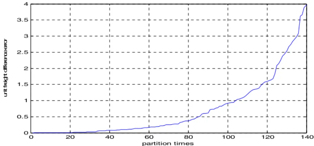
ηand demand forecasting errorβ value were big enough, MATLAB program could cal-culate out all region division results. In the present article, we chose the region division results from times 1 to 140. and traced out the trend of demand forecasting error vary-ing with division times, as shown in Fig. 1; and the trend of unit freight difference error varying with division times, as shown in Fig. 2.

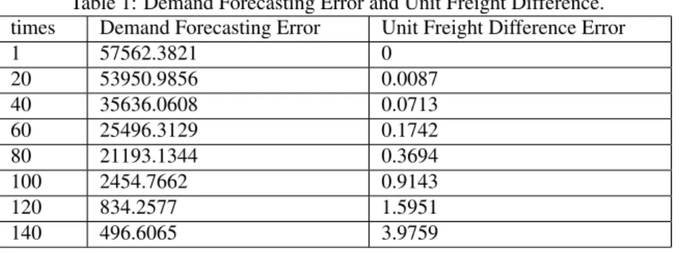
The MATLAB results showed that, at the first time of division, each customer con-sisted of a separate sales region, we had the greatest number of sales regions, the demand forecasting error was as large as 57562.3821 and the unit freight difference error was 0 (see table 1), whereas at the 140 divisions, the demand forecasting error was reduced to 496.6065, and unit freight difference error was enlarged to 3.9759. As shown in Fig.1, we could see that the demand forecasting error decreased in the division times, which shows the method could efficiently enhance the forecasting accuracy. However, as shown in Fig.2, the unit freight error also increased in the division times accumulated.

Table 1: Demand Forecasting Error and Unit Freight Difference. times Demand Forecasting Error Unit Freight Difference Error

1 57562.3821 0 20 53950.9856 0.0087 40 35636.0608 0.0713 60 25496.3129 0.1742 80 21193.1344 0.3694 100 2454.7662 0.9143 120 834.2577 1.5951 140 496.6065 3.9759

The case of NSC illustrated that neither too few nor too many divisions were desir-able: too few divisions would lead to big forecasting errors, resulted from the volatile demands from small size areas, whereas too many divisions would lead to huge freight

0 20 40 60 80 100 120 140 0 1 2 3 4 5 6x 10 4 partiton times d e m a n d f o re c a s ti n g e rr o r

Figure 1: Change Trends of Demand Forecasting Error

difference from one distribution center to each customers within the same sales region. As a result, the estimate on the total freight in that area would be affected. To draw up a better dispatching plan, it was necessary to select appropriateηandβin accordance with specific situation of their own, so as to get a proper sales region division results based on the above-mentioned method.

0 20 40 60 80 100 120 140 0 0.5 1 1.5 2 2.5 3 3.5 4 partition times u n it f re ig h t d if fe re n c e e rr o r

Figure 2: Change Trends of Unit Freight Difference Error

5 Conclusion

In the present paper, we proposed a new method of enhancing logistics demand fore-casting accuracy by means of sales region division, and we discussed the problem of petroleum product demand forecasting in NSC. With the help of MATLAB program, our study illustrated that the region division method could greatly improve forecasting ac-Improvement of Demand Forecasting Accuracy 445

curacy efficiently. In addition, users could select region dividing results freely based on their specific situation. We therefore believed that our method is of great practical value for users.

References

[1] George E.P. Box, Gwilym M. Jenkins, Gregory C. Reinsel, 1999.Time Series Analysis: Fore-casting and Control. China Statistics Press.

[2] Latif. Abdul, King. Maxwell L, 1993. Linear regression forecasting in the presence of AR (1) disturbances.Journal of Forecasting,12(6) 513-524.

[3] Corolyn E Clark, Paul L Foster, Karen M Hogan, George H Webster, 1997. Judgmental ap-proach to forecasting bankruptcy.The Journal of Business Forecasting Methods & Systems, 16(2) 14 -18.

[4] M Mao, E C Chirwa, 2005. Combination of grey model GM (1, 1) with three-point moving average for accurate vehicle fatality risk prediction.International Journal of Crashworthiness, 10(6) 635-642.

[5] James H. Stock, Mark W, 2004. Combination forecasts of output growth in a seven-country data set Watson.Journal of Forecasting, 23(6) 405-430.

[6] Luh-Yu (Louie) Ren, 2007. Revised Mean Absolute Percentage Errors (Mape) for Independent Normal Time Series.Journal of American Academy of Business, 10(2) 65-70.

[7] Michael W. Babcock, Xiaohua Lu, 2002. Forecasting inland waterway grain traffic. Trans-portation Research, Part E (38) 65-74.

[8] Gardner, Everette S., Jr., McKenzie, Ed., 1989. Seasonal Exponential Smoothing With Damped Trends.Management Science, 35(3) 372-376.