Optimizing Sort in Hadoop using
Replacement Selection
Pedro Martins Dusso1,2, Caetano Sauer1, and Theo H¨arder1
1 Technische Universit¨at Kaiserslautern, Kaiserlautern, Germany 2
Universidade Federal do Rio Grande do Sul, Porto Alegre, Brazil
Abstract. This paper presents and evaluates an alternative sorting component for Hadoop based on the replacement selection algorithm. In comparison with the default quicksort-based implementation, replace-ment selection generates runs which are in average twice as large. This makes the merge phase more efficient, since the amount of data that can be merged in one pass increases in average by a factor of two. For almost-sorted inputs, replacement selection is often capable of sorting an arbitrarily large file in a single pass, eliminating the need for a merge phase. This paper evaluates an implementation of replacement selection for MapReduce computations in the Hadoop framework. We show that the performance is comparable to quicksort for random inputs, but with substantial gains for inputs which are either almost sorted or require two merge passes in quicksort.
Keywords: Sorting, Quicksort, Replacement Selection, Hadoop
1
Introduction
This work implements and evaluates an alternative sorting component for Hadoop based on the replacement selection algorithm [9]. Sorting is used in Hadoop to group the map outputs by key and deliver them to the reduce func-tion. Because of Hadoop’s big data nature, this sorting procedure usually is an external sorting. The original implementation is based on the quicksort algo-rithm, which is simple to implement and efficient in terms of RAM and CPU.
Sorting performance is critical in MapReduce, because it is not trivially par-allelizable as map and reduce tasks. The data is parallelized by partitions on the reduce key value, but this requires a lot of data movement. The sort stage of a MapReduce job is network- and disk-intensive, and often reading a page from the hard disk takes longer than the time to process it. Thus, CPU instructions stop being the unit to measure the cost in the context of external sorting, and we replace it by the number of disk accesses—or I/O operations—performed. This difference makes algorithms designed only to minimize CPU instructions not so efficient when analyzed from the I/O point of view. This means that the superiority of quicksort for in-memory processing may not be directly manifested in this scenario.
Our goal in this paper is to assess replacement selection for sorting inside Hadoop jobs. To the best of our knowledge, this is the first approach in that direction, both in academia and in the open-source community. We observe that our implementation performs better for almost-sorted inputs and for inputs that are considerably bigger than the available main memory. Furthermore, it exploits multiple hard drives for better I/O utilization.
The remainder of this work is organized as follows. Section 2 reviews related work and motivates the use of replacement selection. Section 3 reviews algo-rithms for disk-based sorting, focusing on the replacement selection algorithm. In Section 4, we discuss implementation details. First, we present the internals of Hadoop, focusing on the algorithms and data structures used to implement external sorting using quicksort. Second, we present a custom memory manager used to manage the space in the sort buffer in main memory efficiently. Third, we present optimizations in the key comparison during the sort and finally a cus-tom heap with a byte array as the placeholder for the heap entries. In Section 5, we compare our replacement selection method against the original quicksort. Fi-nally, Section 6 concludes this paper, providing a brief overview of the pros and cons of our solution, as well as discussing open challenges for future research.
2
Background
Data management research has shown that replacement selection may deliver higher I/O performance for large datasets [11, 10] in the context of traditional DBMS applications. Replacement selection is a desirable alternative for run gen-eration for two main reasons: first, it generates longer runs than a standard external-sort run-generation procedure. As Knuth remarks in [9], “the time re-quired for external merge sorting is largely governed by the number of runs produced by the initial distribution phase”. The fact that the lesser number of runs created by replacement selection leads to a faster merger phase is also reported in [7]. Thus, to decrease the time required for the merge phase, we increase the size of the runs.
As a second advantage, this algorithm performs reads and writes in a con-tinuous record-by-record process and, hence, it can be carried out in parallel. This is particularly advantageous if a different disk device is used for writing runs because heap operations can be interleaved with I/O reads and writes asynchronously [7]. These optimizations are not possible with quicksort, which operates in a strict read-process-write cycle of the entire input.
A potential disadvantage of replacement selection compared to quicksort is that it requires memory management for variable-length records. Replacement selection is based on the premise that when we select the smallest record from the sort buffer in main memory, we can replace it with the incoming record. In practice, this premise does not hold because variable-length records are the rule and not the exception. When a record is removed from the sort workspace, the free space it leaves must be tracked for use by following input records. If a new input record does not fit in the free space left by the last selection, more records
must be selected until there is enough space. This leads to another problem, namely the fragmentation of memory space. Thus, managing the space in the sort buffer efficiently when records are of variable length becomes a necessity. To address this issue, we implemented a memory manager based on the design proposed by P. Larson in [10]. These characteristics will be evaluated empirically in Section 4.
Run generation in quicksort is a simple, nevertheless effective, strategy to create the sorted subfiles. First the records from the input are read into main memory until the available main memory buffer is full. These records are then sorted in-place using quicksort. Finally, they are written into a new temporary file (run). If we assume fixed-length records such that m records fit in main memory, this process is repeated s
m times, resulting in r := s
m runs of size m stored in the disk.
Another advantage of quicksort is the vast research effort dedicated to it dur-ing the last decades [1, 7, 14, 2]. We call attention to the work in AlphaSort [13], which is a sort component that enhances quicksort with CPU cache optimiza-tions. Two of these techniques include the minimization of cache misses and the sorting of only pointers to records rather than whole records, which minimizes data movements in memory. The reason behind the adoption of quicksort in Al-phaSort is “it is faster because it is simpler, makes fewer exchanges on average, and has superior address locality to exploit the processor caching” [13]. These techniques are also employed by Hadoop in its quicksort implementation. In Section 4.3 we discuss these techniques in the context of replacement selection.
3
Replacement selection sort
Sort algorithms can be classified into two broad categories. When the input set fits in main memory, aninternal sort can be executed. If the input set is larger than main memory, an external sort is required. Memory devices slower than main memory (e.g., hard disk) must work together to bring the records in the desired ordering. We call a sorted subfile arun. The combination of sorting runs in memory followed by an external merge process is described in two phases:
run generation, where intermediary sorted subfiles (i.e., runs) are produced, and
merge, where multiple runs are merged into a single ordered one.
Arecordis a basic unit for grouping and handling data. Akey is a particular field (or a subset of fields) used as criterion for the sort order. Avalueis the data associated with a particular key, i.e., the rest of the record. Whether key and value are disjoint or one is a subset of the other is irrelevant for our discussion.
3.1 Run generation
The replacement selection technique is of particular interest because the ex-pected length of the runs produced is in average two times the size of available main memory. This estimation was first proposed by E.H. Friend in [5] and later
described by E.F. Moore in [12], and is also described in [9]. In real-world ap-plications, input data often exhibits some degree ofpre-sortedness (i.e., there is a correlation between the input and output orders). For instance, the order in which products are ordered from a retail warehouse is closely correlated to the order in which they are delivered. Thus, re-ordering a dataset from one criterion to the other would require only small dislocations in the position of each record. Replacement selection exploits this fact by trying to perform such movements within an in-memory data structure. In such cases, the runs generated by re-placement selection tend to contain even more than 2mrecords. In fact, for the best case scenario, namely when all records can be ordered by dislocating no more thanmpositions, wheremis the number of records that fit in main mem-ory, replacement selection producesonly one run. This means that an arbitrarily large file can be sorted in a single pass.
Step Memory contents Output
1 503 087 512 061 061 2 503 087 512 908 087 3 503 170 512 908 170 4 503 897 512 908 503 5 (275) 897 512 908 512 6 (275) 897 653 908 653 7 (275) 897 (426) 908 897 8 (275) (154) (426) 908 908 9 (275) (154) (426) (509) (end of run) 10 275 154 426 509 154 11 275 612 426 509 275
Table 1: Run generation with replacement selection
Assume a set of tuples
hrecord, statusi, where record is a record read from the unsorted input and status is a Boolean flag indicating whether the record is
active or inactive. Active records are candidates for the current run while inactive records are saved for the next run. The idea behind the algorithm is as follows: assuming a main memory of size m, we read m records from the unsorted input data, setting its status to active. Then, the active tuple with the smallest key is selected and moved to an output file. When a tuple is moved to the output (selection), its place is occupied by another tuple from the input data (replacement). If the record recently read is smaller than the one just written, its status is set to inactive, which means it will be written to the next run. Once all tuples are in the inactive state, the current run file is closed, a new output file is created, and the status of all tuples is reset to active.
We introduce an example from Knuth [9] in Table 1 to explain in detail the replacement selection algorithm. Assume an input dataset consisting of twelve records with the following key values: 061, 512, 087, 503, 908, 170, 897, 275, 653, 426, 154, 509 and 612. We represent the inactive records in parentheses. To select the smallest current record, Knuth advises in [9] to make this selection by comparing the records against each other (in r−1 comparisons) only for a small number of records. When the number of records is larger than a certain threshold, the smallest record can be determined with fewer comparisons using
a selection tree. In this case, a heap data structure can be employed. With a selection tree, we need only log(r) comparisons, i.e., the height of the tree.
In Step 1, we load the first four records from the input data into the memory. We select 061 as the lowest key value, move it to the output and replace the whole record with a new record with key value 908. The lowest key value then becomes 087, which is moved to the output and replaced with 170. The just-added record is also the smallest in Step 3, so we move it out and replace it with 897. Now we have an interesting situation: when the record 503 is replaced, the record read from the input is 275, which islower than 503. Thus, since we cannot output 275 in the current run, it is set as inactive—a state that will be kept until the end of the current run. Steps 6, 7, and 8 normally proceed until we move out record 908, which is replaced by 509. At this point, in Step 9, all records in memory are inactive. We close the current run (with twice the size of the available memory), revert the status of all records to active, and continue the algorithm normally.
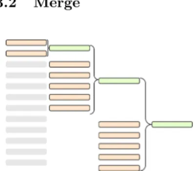
3.2 Merge
Fig. 1: Merging twelve runs into one with merging factor of six.
The goal of the second phase of external sorting, namely the merge phase, is to cre-ate a final sorted file from the existing runs. A heap data structure is used to select the smallest record among all runs, in the exact same way as done in run generation with re-placement selection. A second improvement over the na¨ıve procedure is to take advan-tage of read and write buffers. Givenr runs and memory of sizem, a read buffer of size
m
r+1 can be used for each input run. The size of the write buffer is thenm−( m
r+1)r. Assume that the minimum buffer size isb. If the first phase of the algorithm produces more than mb −1 runs, then we cannot merge these runs in a single step. A natural solution for this limitation is to repeat the merging procedure on the merged runs, producing a merge tree. Figure 1 shows an example of merge tree. At each iteration, mb −1 runs are merged into a new sorted run. The result is r−m
b + 2 runs for the next iteration—the total number of runs minus the merged runs in this turn plus the new merged run. Several heuristics exist to merge runs in such a way that the resulting tree yields minimum I/O cost, such as cascade and polyphase merges, and can be found in [9, 6].
4
Implementation
In this section, we discuss details of our implementation, in which the open-source Hadoop framework was extended with a new sort component. First, we present the internals of Hadoop, focusing on the algorithms and data structures used to implement external sorting using quicksort. Second, we present a custom
memory manager used to manage the space in the sort buffer efficiently. Third, we present optimizations in the key comparison during the sort as well as a memory-efficient customized heap data structure.
4.1 Hadoop internals
In this section, we provide a brief review of the internal components involved in a MapReduce computation in Hadoop. A primary goal of our design is to reuse this infrastructure as much as possible, supporting the replacement selection algorithm in a pluggable way. A detailed analysis of Hadoop’s architecture and the components involved during the execution of a MapReduce job in Hadoop can be found in [3].
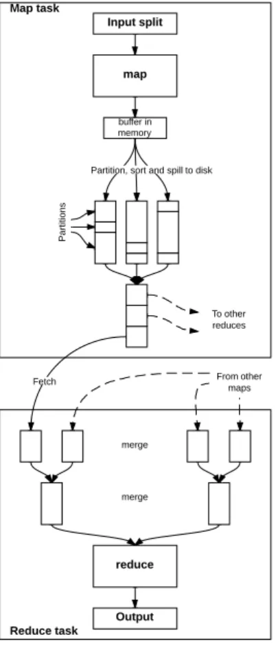
The following process happens in a pipelined fashion, i.e., as soon as one step finishes, the next can start using the output emitted by the former. Figure 2 il-lustrates the process. The map function emits records (key-value pairs) while its input partition is processed, and these records are separated into partitions corresponding to the reducers that they will ultimately be sent to. However, the map task does not directly write the intermediary results to disk. The records stay in a memory buffer until they accumulate up to a certain minimum thresh-old, measured as the amount of occupied space in a buffer called kvbuffer; this threshold is by default 80% the size of kvbuffer. Hadoop keeps track of the records in the key-value buffer in two metadata buffers called kvindices
and kvoffsets. When the buffer reaches the threshold, the map task sorts and flushes the records to disk. When sorting kvoffsets, quicksort’s compare
function determines the ordering of the records accessing directly the partition value in kvindices through index arithmetic. But quicksort’s swap function only moves data in the kvoffsetsbuffer. This corresponds to the pointer sort technique to be discussed in Section 4.3.
When the records are sorted, the map task finally writes them to a run file (or
spill file, in the Hadoop nomenclature). Every time the memory buffer reaches the threshold, the map task flushes it to the disk and creates a new spill. When the map function completes processing the input partition and finishes emitting the key-value pairs, one last spill is executed to flush the buffers. Because the input split normally is larger than the memory buffer, when the map task has written the last key-value, several runs could be present. The map task then must externally merge these spill files into a final output file that becomes available for the reducers. Just like the spill files, this final output file is ordered by partition and, within each partition, by key.
After the completion of a map task, each reduce task (possibly on a different node) copies its assigned slice into its local memory. However, as long as this
copyphase is not finished, the reduce function may not be executed since it must wait for the complete map output. Typically, the copied portion does not fit into the reduce task’s local memory, and it must be written to disk. Once all map outputs are copied, a cluster-wide merge phase begins. As we noted in Section 3.2, if we have more than m−1 map task outputs, the reduce cannot merge the intermediary results of all maps at the same time. The natural solution
is to merge these spills iteratively. Hadoop implements an iterative merging procedure, where the property io.sort.factor specifies how many of those spill files can merged into one file at a time. The details underlying Hadoop’s iterative merging procedure can be found in [3].
Fig. 2: M/R tasks in detail
Hadoop’s sort component not only has to take care of sorting in-memory keys and par-titions but also merge these multiples sorted spills into one single, locally-ordered file. It has to consider data structures carefully to store the records and algorithms to manage and reorder these records. It should be clear that this merge is only a local merge (per-formed by each map task). A second, cluster-wide merge performed on the reduce side will merge the locally-ordered files that each map task has processed. This global merge is be-yond the scope of this work because its per-formance is dictated only by the size and number of runs generated, and it is thus in-dependent of the in-memory sort algorithm. Therefore, our analysis will consider a single merge phase, regardless of whether it is local or global.
4.2 Memory management
As introduced in Section 2, replacement se-lection needs a memory manager to man-age the space in the buffer efficiently when records are of variable length. It is impor-tant to emphasize that memory management is not an issue in Hadoop’s quicksort strat-egy because it only requires swapping records into main memory. This means that a set of records is loaded into main memory and sortedin-place without requiring additional space.
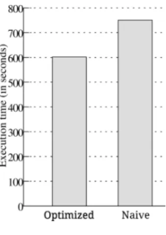
Our na¨ıve implementation simply uses Java’s PriorityQueue class to imple-ment the selection tree. Both memory manageimple-ment and heap impleimple-mentation are reused from Java’s standard library. However, this approach is inefficient due to the JVM’s garbage collection overhead. To eliminate this overhead, we implemented a custom memory manager based on the first-fit design proposed by Larson in [10]. Other alternatives like the best-fit approach proposed in [11] exist, but the evaluation of its efficacy is left for future work. The performance gains of the customized memory manager are shown in the experiment of Fig-ure 3, where run generation is performed for an input of 9GB and a buffer of 16MB. The optimized implementation is approximately 20% faster than the na¨ıve, Java-based implementation.
Fig. 3: Comparion of buffer implementations In our implementation, the sort buffer is divided
intoextents, and the extents are divided intoblocks
of a predetermined size. The block sizes are spaced 32 bytes apart, which results in blocks of 32, 64, 96, 128, and so on. The extent size is the largest possible block size, which is 8KB in our implementation.
For each block size, we keep a list containing all free blocks of that particular size. The number of free lists is given by the extent size divided by the block size, thus 8×1024/32 = 256. The memory manager provides two main methods: one toallocate
a memory block big enough to hold a record of a given size, and one tofree a block that is not in use anymore (i.e., a block just selected for output).
Allocating a memory block big enough to hold a given record means to locate the smallest (we want
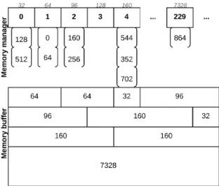
to avoid waste at maximum) free block larger than the record size. The allo-cate method works as follows: round up the record size to next multiple of 32 (drecordSize/blockSizee ∗blockSize). Find the index of the resulting rounded size in the free lists (roundedSize/blockSize−1). Check if the list at the calcu-lated index has a free block: if it does, return it. Otherwise, increment the index and look in the next list (which will be 32 bytes larger). If no block with the rounded record size is found, a larger block is taken and carved to the appropri-ate size, returning the excess as a smaller free block on its appropriappropri-ate list. For instance, in the initial case where there is only one free block of 8192 bytes (the extent size), suppose the memory manager must allocate a block for a record of size 170. The rounded size of 170 is 192; because all other lists are empty, the manager gets the 8192 block from its list. To avoid a major wasting, the 192 first bytes of the 8192 block are returned, and the other 8000 are placed in its appropriate list. When the record is spilled from the buffer and its memory block becomes free, we return the block to the appropriate list. We illustrate this process in the example of Figure 4, which shows a possible buffer state after a sequence of allocate and free invocations.
All lists start initially empty except the last one, which points to blocks of maximum size. As the blocks are allocated and freed, the lists are populated with smaller blocks. In the example of Figure 4, we have 10 blocks of variable sizes. The block sizes are shown inside the blocks in the main-memory buffer (lower part of the figure) and on top of the free list they belong to (upper part of the figure). As smaller records are freed, the allocation process becomes faster, as fewer lists have to be searched to find smaller blocks.
However, this can lead to the following situation. Without loss of generality, imagine that the memory manager is continuously being asked for records of 32 bytes. After 256 block requests—the amount of blocks with 32 bytes in an 8KB extent—assume 4 contiguous (i.e., physically adjacent) blocks are freed. At this point, the memory manager has 128 bytes of free memory fragmented into
four blocks of 32 bytes. If this stream of small records is interrupted by a larger record with 96 bytes, the memory manager will not find any block sufficiently large for that record—despite having enough free memory to answer the request. To remedy this situation, adjacent free blocks must be detected and coalesced
into a single free block of total size equal to the sum of their sizes. For example, a block of 192 bytes being freed next to a free block of 64 bytes can be coalesced into a block of 256 bytes. Such coalescence also requires updating the free lists accordingly.
Fig. 4: A possible state of the memory manager and its free lists
Detecting adjacent free blocks requires special free/occupied markers at the beginning and end of blocks. When a block is freed, the markers of the neigh-boring blocks are verified, and coalescence occurs if either neighbor has a free marker. Because implement-ing this technique is not a trivial task, especially in a memory-managed language like Java, we chose a sim-pler implementation without block coalescence. Instead, we perform a global defragmen-tation operation when large records cannot be allocated. As we show in Section 5, our implementation still delivers superior results than quicksort for the targeted cases, despite the defragmentation penalty.
4.3 Pointer sort
As introduced in Section 2, one of the main advantages of quicksort is thepointer sort technique used to move fewer data. However, Nyberg et al. [13] state that “pointer sort has poor reference-locality because it accesses records to resolve key comparisons”. In an ideal scenario, the whole selection tree should fit on the CPU data cache. But, in practice, the keys used to resolve record comparisons may be too large to fit all at the same time in the data cache. Nyberg et al. suggest the use of a prefix of the key rather than the full key to minimize cache misses. The idea is that a small prefix of the sort key (e.g., 2 bytes) is usually enough to resolve the vast majority of comparisons [7]. The complete record only has to be accessed in the rare occasions in which the prefixes are equal. Further techniques for key normalization and key reordering exist as in [8] and should be evaluated in future work.
We implement this technique ofpointer sorting with key prefixes by storing only a pointer and a key prefix in the heap data structure. The pointer refers to
the block allocated for the record in the memory manager, as discussed above. Since the entries in the heap are of fixed size, we optimized the algorithm even further by implementing a custom heap instead of using Java’s PriorityQueue.
4.4 Custom heap
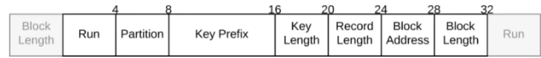
Despite the customized memory manager for records, the JVM is still in charge of managing entries in the heap data structure (i.e., the selection tree). Our objective is to eliminate as far as possible the creation of objects in JVM’s heap space during runtime, and allocate every needed array or object as soon as possible. One of the main advantages of custom managed memory buffer was the serialization of keys and values in a byte buffer of fixed size. To achieve the same result but for the selection tree, we implemented a custom heap which employs a byte array as the placeholder for the heap entries. We illustrate the idea in Figure 5, which shows the format of entries in the optimized heap. We use Java’s
ByteBuffer class to wrap the byte array, which provides methods such putInt
andgetInt, as well similar methods to set and get other data types in arbitrary positions in the byte array. When we add a record to the sort buffer, we add its metadata “heap entry object” by directly writing the run, partition, etc., into the custom heap byte array. With this design, we can directly control how much memory the selection tree will consume, pre-allocating the heap space in a single contiguous block.
Fig. 5: The format of entries in our optimized heap
5
Experiments
This section evaluates the performance of replacement selection in the context of actual Hadoop jobs. First, we evaluate the run generation process, i.e., in-memory sorting using quicksort vs. replacement selection. Our goal is to show that (i) replacement selection indeed generates less runs, and (ii) the efficiency of replacement selection is not much worse than quicksort, i.e., the gains made at the merge phase are not wasted in a slower run generation phase. In fact, when able to exploit the continuous run generation characteristic of replacement selection, described in [7], where reads and writes overlap as the input is con-sumed and the output is produced, replacement selection outperforms quicksort. Second, we take a look at the special case of inputs with a certain degree of pre-sortedness, which is where replacement selection is preferred to quickdort. These experiments are executed as micro-benchmarks to isolate sort performance on a single machine. Finally, in the third experiment set, we execute a full Hadoop job in a cluster comparing the run time with both sorting algorithms.
5.1 Run Generation
To confirm the prediction that replacement selection generates less runs empiri-cally, we ran an experiment with thelineitemtable from the TPC-H benchmark [15]. To randomize the sort order on the input, we consider a lineitem table sorted bycomment, and them used the columnshipdate as sorting key. Since the comment field is generated randomly by the benchmark, no correlation to the ship date is expected.
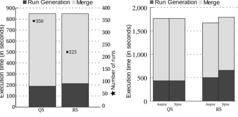
(a) Exec. time and number of runs (b) Performance with two disks Fig. 6: Experiment results for random inputs
Results for this experiment are presented in Figure 6a. The buffer size used in these experiments is 50MB, of which 10% are overheads of auxiliary data structures (e.g., key prefixes). The table size is 700MB, which yields a ratio of 14 between input and buffer size. As shown in the graph, the run generation phase in replacement selection takes a little longer, but it produces approximately two thirds of the number of runs in quicksort. Note that the merge time is approximately the same, despite the substantial difference in the number of runs. This is expected because, in both cases, one merge pass was enough to produce a single sorted output. In this case, replacement selection yields only marginal gains in terms of CPU overhead in the merge phase, which are due to the smaller size of the heap used to merge the inputs. Nevertheless, the goal of this experiment is to show that replacement selection delivers comparable performance to quicksort when inputs are randomly ordered, which is clearly shown in the results. It substantially outperforms quicksort when inputs have a certain degree of pre-sortedness or, similarly, when multiple passes are required in quicksort. These cases are analyzed in Sections 5.2 and 5.3 below.
The quicksort algorithm exhibits a fixed read-process-write cycle that does not allow I/O overlapping. One of the advantages of replacement selection is the continuous run generation process, alternately consuming input records and
producing run files [7]. To demonstrate this fact empirically, we extended Hadoop with an asynchronous writer following the producer-consumer pattern. The idea is to place sorted blocks of data into a circular buffer instead of writing them directly to disk. Then, an asynchronous writer thread consumes blocks from this buffer and performs the blocking I/O write. While it waits, the sorting thread can sort other blocks of data in parallel. The results of our experiment are shown in Figure 6b, where we compare the elapsed time of run generation with two hard disks—one for input and one for output. As predicted, quicksort delivers the same performance regardless of whether the writer is synchronous or asynchronous, whereas replacement selection benefits from writing asynchronously, performing run generation approximately 30% faster. This is because reads from one disk are performed in parallel with writes on another disk. Using the asynchronous writer, the performance of replacement selection approximates that of quicksort, despite the higher overheads of heap operations and memory management.
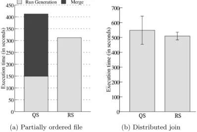
(a) Partially ordered file (b) Distributed join
Fig. 7: Experiment results for pre-sorted input and join computation
5.2 Exploiting Pre-sortedness
One of the major advantages of replacement selection is that it can exploit pre-sortedness on the input file. Estivill-Castro and Wood showed mathematically in [4] that the length of the runs created by replacement selection increases as the order in the input file increases. To confirm this prediction empirically, we ran an experiment with thelineitem table again. We took as input the lineitem table sorted by shipdate, using the column receiptdate as new sorting key. We prepared the table by sorting the file byshipdatebeforehand, but in practice this scenario could also occur if there is a clustered index or materialized view on
shipdate. Since there is a strong correlation between the dates on which orders are shipped and received, this constitutes a good example of pre-sorted input.
The input dataset used in this experiment is the same as on the experiment of Figure 6a, but with a different pre-sort order. As shown, the run generation phase takes considerably longer with replacement selection, but it produces only a single run at the end, meaning that no merge phase is required. As predicted, replacement selection acts as a sort sliding-window in this case. Note that quick-sort finishes run generation earlier, but an additional pass over the whole input is required in the merge phase, requiring about 35% more time in total.
5.3 Distributed Join
To conclude the experiments, we created a test scenario where a distributed join of two TPC-H tables is performed. Joins are a common operation in data management systems, and in MapReduce both inputs must be sorted by the join key (i.e., a sort-merge join algorithm). The joined tables arelineitem, which has about 1GB, andorders, with 600MB. This experiment was performed in a small cluster running Hadoop 2.4.0 with six nodes and we measured the total execution time of the jobs. The buffer size was 16MB, which yields a 62.5 ratio with the lineitem table and a 37.5 ratio with the order table. Note that despite the tables being relatively small for typical Hadoop scales, the determinant factor for performance is actually the ratio between input and sort buffer size. A real-world large scale scenario would probably deal with sizes up to 1000×larger, i.e., tables of 1TB and 600GB, and a sort buffer of 16GB. In such situations, the relative performance difference between the two algorithms would be very close to what is observed in our experiment, because the ratio is the same. The results in Figure 7b confirm our expectation that replacement selection is faster, because less runs are generated. Furthermore, it seems that it is also more robust in terms of performance prediction, given the lower standard deviation.
6
Conclusion
This work described the implementation and evaluation of an alternative sort component for Hadoop based on the replacement selection algorithm. The orig-inal implementation, based on quicksort, is simple to implement and efficient in terms of RAM and CPU. However, we demonstrated that under certain condi-tions, such as pre-sorted inputs and large ratio between input and memory size, replacement selection is faster due to the lower number of runs to be merged. For the remaining cases, we showed that the performance is very close to that of quicksort, meaning that the average long-term gain in a practical scenario is in favor of replacement selection.
Despite the demonstrated advantages of replacement selection, we believe the implementation has the potential to outperform quicksort even further with certain optimizations. The main task in that direction is to optimize the main memory management component (e.g., by implementing block coalescence [10])
and the heap data structure (e.g., by minimizing the number of comparisons with a tree-of-losers approach or by optimizing key encoding [9, 7, 8]). Our work has been published as an open source pluggable module for Hadoop3. We hope to implement the mentioned optimizations and improve our code to integrate it with the official Hadoop distribution.
Acknowledgements
We thank Renata Galante for her helpful comments and suggestions on earlier revisions of this paper.
References
1. Bentley, J.L., Sedgewick, R.: Fast algorithms for sorting and searching strings. In: Proceedings of the Eighth Annual ACM-SIAM Symposium on Discrete Algorithms. pp. 360–369. SODA ’97, SIAM, Philadelphia, PA, USA (1997)
2. Cormen, T.H., Leiserson, C.E., Rivest, R.L., Stein, C.: Introduction to Algorithms, Third Edition. The MIT Press, 3rd edn. (2009)
3. Dusso, P.M.: Optimizing Sort in Hadoop using Replacement Selection. Master thesis, University of Kaiserslautern (2014)
4. Estivill-Castro, V., Wood, D.: Foundations for faster external sorting (extended abstract). In: Thiagarajan, P.S. (ed.) FSTTCS. LNCS, vol. 880, pp. 414–425. Springer, Heidelberg (1994)
5. Friend, E.H.: Sorting on electronic computer systems. J. ACM 3(3), 134–168 (Jul 1956)
6. Graefe, G.: Query evaluation techniques for large databases. ACM Comput. Surv. 25(2), 73–169 (Jun 1993)
7. Graefe, G.: Implementing sorting in database systems. ACM Comput. Surv. 38(3) (Sep 2006)
8. H¨arder, T.: A Scan-driven Sort Facility for a Relational Database System. In: Proc. VLDB. pp. 236–244 (1977)
9. Knuth, D.E.: The Art of Computer Programming, Volume 3: (2Nd Ed.) Sorting and Searching. Addison Wesley Longman Publishing Co., Inc., Redwood City, CA, USA (1998)
10. Larson, P.A.: External sorting: Run formation revisited. IEEE Transactions on Knowledge and Data Engineering 15(4), 961–972 (Jul 2003)
11. Larson, P.A., Graefe, G.: Memory management during run generation in external sorting. In: Proceedings of the 1998 ACM SIGMOD International Conference on Management of Data. pp. 472–483. SIGMOD ’98, ACM, New York, NY, USA (1998)
12. Moore, E.: Sorting method and apparatus (May 9 1961), http://www.google.com.br/patents/US2983904
13. Nyberg, C., Barclay, T., Cvetanovic, Z.: AlphaSort: A RISC machine sort. In: Proc. SIGMOD. pp. 233–242 (1994)
14. Skiena, S.S.: The Algorithm Design Manual. Springer-Verlag New York, Inc. (1998) 15. Transaction Processing Performance Council: TPC Benchmark H (Decision Sup-port) Standard Specification. http://http://www.tpc.org/tpch/, accessed: 2014-01-10
3