ALCOHOL AND HIV SEROCONVERSION IN MEN WHO HAVE SEX WITH MEN
Petra Michelle Sander
A dissertation submitted to the faculty of the University of North Carolina at Chapel Hill in partial fulfillment of the requirements for the degree of Doctor of Philosophy in the
Department of Epidemiology.
Chapel Hill 2011
ii © 2011
iii ABSTRACT
PETRA MICHELLE SANDER: Alcohol and HIV Seroconversion in Men Who Have Sex with Men
(Under the direction of Stephen R. Cole)
Previous findings linking alcohol consumption and HIV seroconversion among men who have sex with men (MSM) have been inconsistent. This study argues those findings may be limited by inadequate control for confounding due to time-updated factors affected by prior alcohol consumption. We examined prospective data from 3,725 HIV-seronegative MSM enrolled in the Multicenter AIDS Cohort Study (MACS). Participants made
semiannual study visits from 1984-2007, self-reported alcohol consumption, and underwent HIV testing. Potential predictors of alcohol consumption were explored. Demographic and time-updated factors including smoking, self-reported depression symptoms, illicit drug use and sexual practices were considered. Associations were modeled using logistic and
lognormal multivariable regression. We next examined the joint effects of alcohol
iv
seroconversions occurred. After accounting for several measured confounders using a joint marginal structural Cox proportional model, the hazard ratio (HR) of HIV seroconversion for moderate drinking (1-14 drinks/week) compared to nondrinking was 1.10 (95% CL: 0.78, 1.54) and for heavy drinking (>14 drinks/week) was 1.61 (95% CL: 1.12, 2.29) compared to nondrinking. The HRs for heavy drinking compared to nondrinking for participants with 0-1 or >1 URAI partner were 1.37 (95% CL: 0.88, 2.16) and 1.96 (95% CL: 1.03, 3.72),
v
ACKNOWLEDGMENTS
Dr. Stephen Cole has been a tremendous mentor and I am incredibly thankful for the opportunity to work on this research with him. He is not only a superb methodologist and scholar, but also a patient and supportive teacher. My thanks also go to the members of the Cole advising group: Dr. Chanelle Howe, Dr. Daniel Westreich, Dr. Karminder Gill, Ashley Naimi, Christina Ludema, Jess Edwards, and Nadya Belenky who graciously provided feedback throughout the development of this dissertation and challenged me to grow as an epidemiologist.
I would also like to acknowledge the other members of my dissertation committee and my co-authors from the Multicenter AIDS Cohort Study (Dr. David Ostrow, Dr. Lisa
Jacobson, Dr. Robert Bolan, Dr. Ron Stall and Ms. Lisette Johnson-Hill) for their comments on this work and support over the past two and a half years. I am grateful for the guidance of all my professors and mentors in the Department of Epidemiology and for the assistance of Nancy Colvin and Carmen Woody.
The members of my dissertation support groups, both formal and informal, have kept me motivated over the past years. Thank you, Dr. Margaret Adgent, Kirstin Huiber, Kim
vi
Finally, I would like to thank my parents for their support during my entire education. None of this would have been possible without them.
Financial support was provided by the National Institute on Alcohol Abuse and Alcoholism (R01-AA-01759, Stephen R. Cole, Principal Investigator). Data in this dissertation were collected by the Multicenter AIDS Cohort Study (MACS) with centers (Principal Investigators) at The Johns Hopkins Bloomberg School of Public Health (Joseph B. Margolick, Lisa P. Jacobson), Howard Brown Health Center, Feinberg School of
vii
TABLE OF CONTENTS
LIST OF TABLES ... ix
LIST OF FIGURES ... xi
LIST OF ABBREVIATIONS ... xii
CHAPTER I. SPECIFIC AIMS ...1
II. BACKGROUND AND SIGNIFICANCE ...4
The HIV epidemic among MSM in the US ... 4
Alcohol consumption in the US ... 5
Literature review ... 6
Alcohol and sexual risk behavior ... 10
Physiologic responses to alcohol ... 13
Significance ... 15
III. METHODS ...23
Study population ... 23
Data collection and measures ... 24
Human subjects ... 25
Statistical methods for aim 1 ... 26
viii
AMONG US MEN WHO HAVE SEX WITH MEN, 1984-2007...44
Introduction ... 44
Materials and methods ... 45
Results ... 49
Discussion ... 52
V. JOINT EFFECTS OF ALCOHOL CONSUMPTION AND HIGH-RISK SEXUAL BEHAVIOR ON HIV SEROCONVERSION AMONG MEN WHO HAVE SEX WITH MEN ...63
Introduction ... 63
Materials and methods ... 64
Results ... 70
Discussion ... 72
VI. CONCLUSIONS ...81
Summary ... 81
Limitations ... 82
Implications ... 83
Future studies ... 84
APPENDICES ...86
Appendix 1. Additional tables ... 86
Appendix 2. Additional figures ... 91
ix
LIST OF TABLES
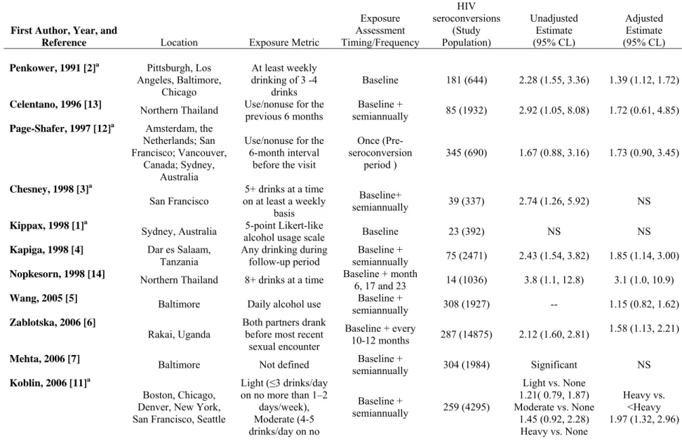
Table 2.1. Prospective studies of alcohol and HIV seroconversion ...17
Table 2.2. The Alcohol Use Disorders Identification Test - consumption questions ...19
Table 2.3. US standard drink ...20
Table 3.1. MACS follow-up visit questionnaire, semiannual visit ...40
Table 3.2. Covariables ...41
Table 3.3. Center for Epidemiologic Studies- depression scale ...42
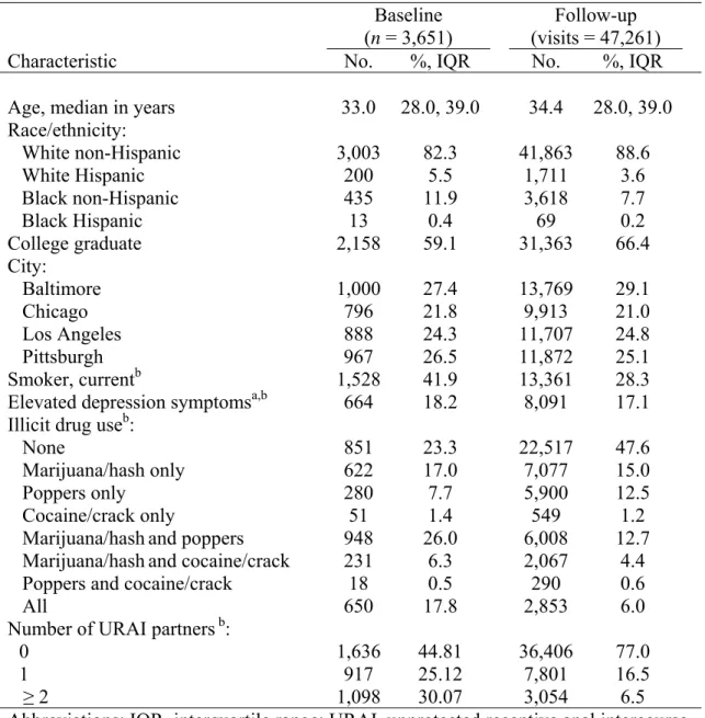
Table 4.1. Characteristics of 3,651 men who have sex with men, 3,651 baseline visits and 47,261 follow-up visits between1984 and 2007. ...57
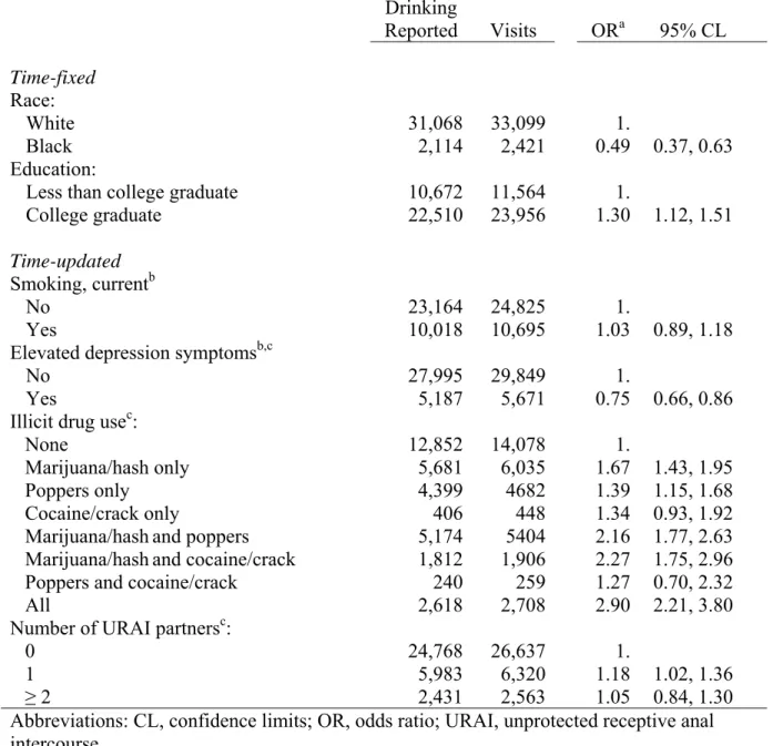
Table 4.2. Report of any current drinking among 3,102 men who reported any drinking at the prior visit, 35,520 visits between 1984 and 2007. ...58
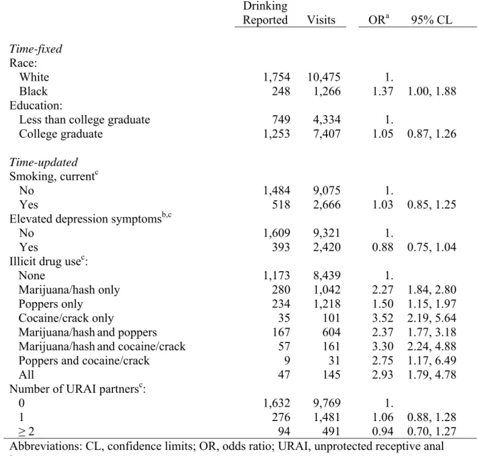
Table 4.3. Report of any current drinking among 1,554 men who reported no drinking at the prior visit, 11,741 visits between 1984 and 2007. ...59
Table 4.4. Number of drinks per week consumed by 2,644 current drinkers, 35,184 visits between 1984 and 2007. ...60
Table 5.1. Enrollment characteristics of 529 Multicenter AIDS Cohort Study HIV seroconverters and 3,196 HIV-seronegative participants ...76
Table 5.2. Effect of alcohol consumption on HIV seroconversion among 3,725 men in the Multicenter AIDS Cohort Study between 1984 and 2007. ...77
Table 5.3. Effects of alcohol consumption and risky sexual behavior in the prior year on HIV seroconversion among 3,725 men in the Multicenter AIDS Cohort Study between 1984 and 2007. ...78
Appendix 1.5.1. Comparison of empirical induction periods ...86
x
Appendix 1.5.3. Characteristics of 529 Multicenter AIDS Cohort
Study HIV seroconverters and 3,196 HIV-seronegative participants studied over 57,651 follow-up visits. ...88 Appendix 1.5.4. Characteristics of Multicenter AIDS Cohort Study
xi
LIST OF FIGURES
Figure 2.1. Distribution of drinking levels, for men 18 years of
age and older: United Status, National Health Interview Survey, 1997-2008 ...21
Figure 2.2. Overview of the association between alcohol consumption and HIV seroconversion ...22 Figure 4.1. Plots showing the proportion of participants abstaining
from alcohol, consuming alcohol at moderate levels (0-14 drinks/week) or at heavy levels (>14 drinks/week) ...61
Figure 5.1. Cumulative incidence of HIV seroconversion between 1984 and 2007 among 3,725 men who have sex with men ...79 Appendix 2.4.1. Plot of alcohol consumption by time-on-study at
baseline and over 47,261 follow-up visits by 3,651 men between 1984 and 2007 ...91
Appendix 2.4.2. Box plots of alcohol consumption by illicit drug use ...92 Appendix 2.5.1. Scatterplot of alcohol consumption (drinks/week)
by number of unprotected receptive anal intercourse partners reported over 57,651 follow-up visits, between 1984 and 2007. ...93
xii
LIST OF ABBREVIATIONS
ACASI audio computer-assisted self-interview ADH alcohol dehydrogenase
AIDS acquired immune deficiency syndrome AUDIT Alcohol Use Disorders Identification Test BAC Blood Alcohol Content
CES-D Center of Epidemiologic Studies – Depression scale CL confidence limit
dL deciliter
g gram
HIV human immunodeficiency virus HR hazard ratio
IQR interquartile range IL interleukin
IPW inverse probability weighting MACS Multicenter AIDS Cohort Study MSM men who have sex with men
OR odds ratio
PBMC peripheral blood monocytes RR relative risk
URAI unprotected receptive anal intercourse
CHAPTER I SPECIFIC AIMS
Introduction
Alcohol consumption is believed to be an upstream determinant of drug use and sexual risk behavior and therefore an indirect determinant of human immunodeficiency virus (HIV) risk; however, little empirical evidence exists to support the latter claim and the possible (immune-modulated) direct effects of alcohol on HIV have not been considered. Findings related to alcohol exposure have been inconsistent [1-14] and therefore insufficient to support increased HIV prevention activities targeted at drinking behavior. The overall goal of this study is to estimate the impact of alcohol consumption on HIV acquisition using quantitative methods that permit the unbiased estimation of causal effects under stated assumptions.
The aims have been undertaken with data from the Multicenter AIDS Cohort Study (MACS), which is based in four United States (US) metropolitan areas: Baltimore,
2
computer-assisted interviews concerning demographic, medical and behavioral data. This observational cohort represents perhaps the best available domestic data source to consider long-term alcohol consumption, which is impossible to assess using a randomized design.
An unbiased and precise estimate of the effect of alcohol consumption on HIV seroconversion is essential to the development of targeted HIV interventions for men who have sex with men and other groups at risk for HIV in which alcohol consumption is common.
Specific aim 1. Estimate the association of measured behavioral and demographic factors with subsequent alcohol consumption.
Hypothesis 1: Baseline demographic factors (e.g., younger age, white race, non-Hispanic ethnicity), prior time-varying high risk health behaviors (e.g., higher number of past sexual partners, higher number of acts of unprotected receptive anal
intercourse, illicit drug use), and prior time-varying biomedical factors (e.g., serious health concerns in the medical history, body-mass index, weakened immune function) will be associated with heavier subsequent alcohol consumption.
Specific aim 2. Estimate the effect of alcohol consumption on the risk of HIV seroconversion.
3
Hypothesis 2.2: Alcohol consumption within the 12 months prior to HIV seroconversion will show a stronger association with HIV seroconversion than alcohol consumption in the 36 months prior to HIV seroconversion.
CHAPTER II
BACKGROUND AND SIGNIFICANCE
The HIV epidemic among MSM in the US
According to 2006 estimates there were 56,300 [15] new HIV infections in the US with MSM transmission accounting for 72% of male seroconverters including 81% of new infections among whites, 63% among Blacks, and 72% among Hispanics [16]. Among MSM, unprotected anal intercourse, particularly unprotected receptive anal intercourse, is the major mode of HIV transmission [17-25] with an estimated per contact infectivity of 0.82% (95%
CL: 0. 24, 2.76) [17]. The friction of anal-penile sexual contact is thought to compromise innate immunity at the mucosal surface by producing micro-tears in the epithelial linings of the rectum and colon, allowing cell-free HIV to be transcytosed into the underlying lamina
propria. There it may locally infect HIV target cells, including submucosal dendritic cells,
Langerhans cells and CD4+ T cells before ultimately spread via the lymph nodes and producing systemic infection [26, 27].
5
the field of HIV treatment adherence research [31, 32], particularly as these activities may lead to physiologic changes that lead to poor prognosis [33] and hasten progression to AIDS [34].
Alcohol consumption in the US
Two-thirds of the US adult population identify as alcohol consumers [35], making alcohol along with caffeine and nicotine, one of the most widely used addictive substances nationally. Moderate to heavy drinkers make up 20% of the drinking population (Figure 2.1), with a smaller proportion of the population reporting heavy (>14 drinks/week for men) or binge (>5 drinks per sitting for men) than in Europe [36]. Among adult males in the general population, alcohol use (i.e., choosing to drink alcohol rather than abstaining) is associated with white race, higher levels of education, younger ages, and being married. Higher levels of alcohol consumption, the number of drinks consumed in a typical day, among those who drink are associated with more recent birth cohort, younger age, periods of higher per capita drinking, being unmarried, non-white race, higher levels of education, non-suburban
residence, smoking, and psychological comorbidities, particularly depression [37, 38]. MSM were historically thought to consume alcohol at rates that exceed the general population. As reviewed extensively by others [39, 40], early studies of alcohol consumption and alcohol-related disorders among MSM observed low abstention rates, high alcohol consumption and smaller age-related declines in alcohol consumption when compared to the general population [41, 42]. However, these studies suffered from bias due to recruitment of homosexuals from alcohol-saturated settings (e.g., gay bars, urban settings) and differential recruitment of MSM and general population participants. Early findings were not
random-6
digit dialing of homosexuals and heterosexuals [40, 43]. Additionally, knowledge of the ongoing HIV epidemic among MSM has corresponded to overall declines in alcohol abuse [44].
Literature review
Three types of studies characterize the existing literature linking alcohol consumption to HIV and sexual risk behavior: general association studies, which consider average
measures of alcohol consumption and resulting outcomes; situational covariation studies that consider the use of alcohol in specific (e.g., sexual) contexts; and event-level analyses that consider risk behavior around the time of an index sexual act [45-50]. When HIV infection is the outcome, the latter study types are subject to differential recall bias, because the precise timing of infection is usually unknown to the study participant and he may preferentially assign the index act to a time at which he engaged in high risk activities. By contrast,
seroconversion, the development of an antibody response by the immune system to HIV, can be detected independent of the participant self-report and is more frequently the outcome in general association studies.
A review of twenty African studies of alcohol consumption which focused primarily on heterosexual HIV transmission and included three prospective studies, reported an
unadjusted pooled odds ratio of 1.70 (95% CL: 1.42, 1.72). While the drinking status of HIV-positive individuals is certainly of interest to the study of predictors of care seeking and treatment adherence, cross-sectional associations are insufficient to support causal
7
interview, indeed high risk behaviors are likely to change following notification [51].
Therefore, subsequent discussion will be limited to studies that gather information on alcohol consumption or use during at least one period prior to HIV diagnosis. This approach assures the temporal order role of alcohol consumption vis-à-vis HIV seroconversion.
To our knowledge, 14 previous studies [1-14] have considered alcohol use prospectively with HIV seroconversion as an outcome in a variety of populations (Table 2.1). These studies report relative unadjusted effect measures between 1.21 (comparing light to nondrinkers [11]) and 4.82 (comparing individuals drinking more than 30 standard
alcoholic drinks per week to nondrinkers [10]). Adjustment for a variety of baseline
8
1.53). Thus, the previous studies on this subject collectively support an association between alcohol consumption HIV risk; however, the causal link between alcohol and HIV
acquisition is an open question due in part to shortcomings as well as the differences observed between studies [52].
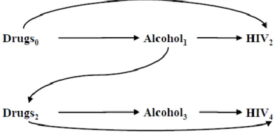
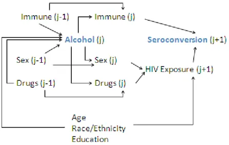
At the time this research was proposed no previous study that included time-varying exposure or covariate levels has appropriately estimated the effect of alcohol on HIV seroconversion as there is confounding by time-dependent covariates (e.g., sexual risk behaviors, immunological health, drug use, etc.), which are determined in part by prior alcohol consumption and both predict HIV seroconversion and subsequent alcohol consumption (Figure 2.2) [53]. Under these conditions traditional adjustment approaches (e.g., regression methods), even those which adjust for time-dependent confounders, may produce biased estimates of the effect estimate of interest [54]. Therefore, the opportunity exists to apply novel techniques [54], which allow for the unbiased estimation of
dependent alcohol consumption on HIV seroconversion, adjusting for both baseline and time-dependent confounding.
Measurements of alcohol consumption in the HIV seroconversion literature
9
literature [58] is also apparent in studies of alcohol consumption and HIV acquisition. Here, Woolf and Maisto warn that “Continuing to take a unitary approach to research design could impede the advancement of knowledge regarding alcohol use and risky sex among MSM. Unfortunately it appears that researchers in this area have done little to obtain empirical evidence on the reliability or accuracy of the self-report data that they do collect” [60].
In the previously cited meta-analyses of alcohol consumption and HIV infection [46, 60], the authors have considered alcohol use as a dichotomous (yes or no) variable,
regardless of the time period covered or if the study queried using a diagnostic instrument such as the Alcohol Use Disorders Identification Test (AUDIT) or its abridged form, the AUDIT-C (Table 2.2), another quantity-frequency questionnaire, or a contextual marker of alcohol consumption, such as living in a home from which alcohol is sold. Similarly, alcohol consumption measurement in prospective studies has relied exclusively on non-validated self-report, and has generally been dichotomized by the authors into categories of ever vs. never or heavy drinker vs. non-heavy drinker using various cut points (Table 2.1). Only the study by Watson-Jones et al. presents adjusted and unadjusted effect measure estimates
10
sexual contact and reflect an “event level” analytic approach. In the study by Kippax et al.
[1], respondents report on the sex act at which they believe they were infected with HIV, a possibly misleading approach due to differential recall. Zablotska et al. [6] consider alcohol
consumption by one or both partners as a risk factor; however, the reported findings do not distinguish which partner was drinking. The drinking status of the HIV negative partner may influence the risk of HIV transmission through behavioral and immunological pathways; Zablotska et al.’s approach, however, would muddy the indirect effects due to biological
changes.
Biomarkers have been applied to assess the validity of self-reported alcohol
consumption by insurance agencies [62], in dependence research [63] and law enforcement, all settings where confidence in accurate self-report is low. No gold standard for measuring moderate to long term alcohol intake exists across all levels of consumption, however personal monitoring of the transdermal or exhaled ethanol to measure a Blood Alcohol Content (BAC) around the time alcohol is imbibed (within 8 hours) is likely the best measure currently available of acute drinking [64]. Both these methods are used, for example, when legal or health concerns warrant heightened vigilance [65]. However, they are costly, intrusive, and measure only short-term consumption.
Alcohol and sexual risk behavior
11
(3-5 drinks), judgment and motor coordination are impaired; at a BAC of 0.20-0.25 (~10 drinks) there are signs of sedation; and at higher levels, loss of consciousness, asphyxiation, coma and death are more likely [67, 68]. Alcohol levels of as low as 0.1 may interfere with maintaining an erection [68]; however, the precise impact of alcohol on sexual function is highly dependent on context [69]. The median lethal dose of ethanol corresponds to a BAC of approximately 0.4-0.5 [67].
In popular opinion, alcohol consumption is a social lubricant associated with an attitude of disinhibition and risk taking, particularly sexual risk taking [70]. This intuitive understanding is borne out by some [71-78], but not all [79-83] epidemiologic investigations of the subject among MSM. Alcohol consumption was associated with higher numbers of sexual partners [84, 85], higher numbers of unprotected anal sex acts, and condom failure [86]. The influence of alcohol was modified by partner type [72, 87, 88] and sexual behavior [74, 89] with casual partners and receptive anal intercourse with individual of unknown HIV status correlating to alcohol consumption prior to sex.
Behavioral scientists have studied this association and posited three theoretical models [23, 90] through which to understand increased individual sexual risk behavior following alcohol use.
Alcoholic myopia, or the ability of alcohol to cloud short-term decision making
12
several population-based cross-sectional studies [81, 93] and an event-level analysis [94] failed to show reduction in condom use when alcohol consumption preceded sex. Indeed, the results suggest that pre-existing behavior patterns were unaltered by drinking [94], and that observed unsafe sex practices under the influence were common to participants who were also inconsistent condom users while sober.
Alcohol expectancy theory posits that individuals drink in anticipation of a heightened
sexual experience [95]. This is supported by research in adolescents that shows alcohol use is associated with earlier initiation of sexual activity and more sexual partners [96-98]. Among MSM, the consumption of alcohol accompanies a desire to cognitively escape from fears of HIV risk [99, 100].
A third behavioral theory suggests that risky sexual behavior and alcohol use may both be expressions of an underlying risk-prone personality type [23, 94, 101]. The presence of a sensation-seeking personality type assessed through survey inquiry into dimensions of
13 Physiologic responses to alcohol
A healthy occasional drinker can metabolize one standard drink (Table 2.3) in one hour. When a person ingests an alcoholic beverage, the ethanol it contains passes into the stomach and intestinal tract, where it may be immediately metabolized by alcohol
dehydrogenase (ADH) isoenzymes. The extent of this first pass metabolism is influenced by the amount of time alcohol remains in the stomach. Unmetabolized ethanol passes from the stomach and intestines into the circulatory system and on to the liver for metabolism. There, ethanol is converted into acetaldehyde by ADH and then from acetaldehyde into acetic acid by aldehyde dehyrodgenase (ALDH). Depending on the needs of the body, acetic acid is further metabolized into carbon dioxide and water or transported to cells outside of the liver. Oxidized nicotinamide adenine dinucleotide molecules act as coenzymes required for the activity of both alcohol metabolizing enzymes. Once reduced, this coenzyme may shuttle the energy from the breakdown of alcohol to other parts of the cell.
Polymorphic variants of the genes that encode alcohol metabolism enzymes are associated with altered kinetic properties. These have been linked to differences in alcohol consumption patterns and may explain some of the disparities observed in alcohol
dependence across races and ethnicities [107, 108]. For example, homozygosity for the
ALDH2*2 allele is associated with low-dose alcohol hypersensitivity (e.g., flushing and
general discomfort) and with a reduced likelihood of heavy drinking and alcoholism in Asians [109, 110]. Similarly ADH variants ADH1B*2 and ADH1B*3, most common among
14
Alcohol consumption has consequences for virtually every part of the body, including the immune system. For example, it is well established that chronic alcohol consumption is associated with increased susceptibility to bacterial infection, including tuberculosis [113]. No confirmed biologic mechanism has been established linking acute or chronic alcohol consumption to HIV infection. Nevertheless, two general hypotheses are currently under exploration in the laboratory: first, that alcohol increases host cell susceptibility to initial HIV infection and second, that once cells are infected, HIV proliferation is enhanced in the
presence of alcohol and may hasten an individual’s progression to AIDS [101].
A study in humans collected peripheral blood monocytes (PBMCs) from six healthy adult volunteers before and after a weekend of social drinking (700 to 3100 ml of beer or an equivalent amount of alcohol in another beverage) and measured the ability of HIV-1 to replicate in the PBMC in vitro [114]. Alcohol consumption was correlated with an increase
in HIV-1 replication in the PBMCs and a decreased ability of these cells to produce cytokines, such as interleukin-2 (IL-2), which regulate the responses of other immune components to the virus-infected cell. A second study applied the same hypothesis as above, this time with 60 healthy volunteers who were asked to engage in “social drinking” over a weekend. In this case, moderate alcohol consumption (53.50g alcohol ± 15.00) greatly increased HIV replication in PBMCs and was associated with decreases in both T-helper and T-suppressor cell function. A reduction in CD8+ T cells in turn leads to an increase in HIV replication in vitro [115].
15
of the CXCR4 receptor [118]. Secondary effects of alcohol exposure include modulation of cytokines released from immune cells: dendritic cell function appears to decline in response to alcohol exposure, leading to a decrease in IL-12 circulation and an increase in IL-10 [119]. Under binge drinking conditions, an increase in pro-inflammatory cytokines was observed [120] alongside an increase in the proportion of HIV-susceptible cells in the circulatory system [121]. Chronic alcohol consumption reduces delayed-type hypersensitivity response [122, 123], decreases the absolute lymphocyte count, reduces macrophage functions [116, 124], increases natural killer cell activity, and increases tumor necrosis factor production
which may in turn increase HIV-1 replication. Among immunized macaques, exposure to simian immune deficiency virus was associated with a hastened SIV-related decrease in CD4+ T cells in alcohol-consuming versus control animals [125].
Significance
Our study of alcohol consumption in the nation’s largest cohort of MSM at risk for HIV infection addresses deficiencies in the current literature and aims to improve upon existing methodological approaches for handling confounding. Our work specifically builds on the contributions of Penkower, et al. [2] who were to our knowledge the first to
investigate alcohol and HIV seroconversion with prospective data drawn from the early waves of MACS. The inability of the field to reach consensus since 1991 speaks to the necessity of this research.
16
unprotected intercourse, a year after entry into alcohol treatment; however, the numbers of observed seroconversions was too small to draw conclusions about that endpoint [126]. Compared to their peers, MSM may be less likely to seek individual treatment for alcohol use disorders [127] and if they do enter, may leave due to limited MSM-specific training of treatment providers or overt homophobia [128]. Community-based HIV prevention interventions targeted specifically at MSM that include modules about negotiating
intercourse under the influence of alcohol but do not directly promote reduced consumption of alcohol have been tested [129, 130]. However, the long-term impact of these interventions is unclear. Community-based interventions in South Africa based on the World Health Organizations’ model of alcohol intervention, which includes motivational and behavioral skills training, have been associated with promising short-term declines in risky sexual practices [131, 132].
17
Table 2.1. Prospective studies of alcohol and HIV seroconversion.
First Author, Year, and
Reference Location Exposure Metric
Exposure Assessment Timing/Frequency HIV seroconversions (Study Population) Unadjusted Estimate (95% CL) Adjusted Estimate (95% CL)
Penkower, 1991 [2]a Pittsburgh, Los
Angeles, Baltimore, Chicago
At least weekly drinking of 3 -4
drinks Baseline 181 (644) 2.28 (1.55, 3.36) 1.39 (1.12, 1.72)
Celentano, 1996 [13] Northern Thailand Use/nonuse for the
previous 6 months
Baseline +
semiannually 85 (1932) 2.92 (1.05, 8.08) 1.72 (0.61, 4.85)
Page-Shafer, 1997 [12]a Amsterdam, the
Netherlands; San Francisco; Vancouver,
Canada; Sydney, Australia
Use/nonuse for the 6-month interval
before the visit
Once (Pre-seroconversion
period ) 345 (690) 1.67 (0.88, 3.16) 1.73 (0.90, 3.45)
Chesney, 1998 [3]a
San Francisco on at least a weekly 5+ drinks at a time basis
Baseline+
semiannually 39 (337) 2.74 (1.26, 5.92) NS
Kippax, 1998 [1]a Sydney, Australia 5-point Likert-like
alcohol usage scale Baseline 23 (392) NS NS
Kapiga, 1998 [4] Dar es Salaam,
Tanzania
Any drinking during follow-up period
Baseline +
semiannually 75 (2471) 2.43 (1.54, 3.82) 1.85 (1.14, 3.00)
Nopkesorn, 1998 [14] Northern Thailand 8+ drinks at a time Baseline + month
6, 17 and 23 14 (1036) 3.8 (1.1, 12.8) 3.1 (1.0, 10.9)
Wang, 2005 [5] Baltimore Daily alcohol use Baseline +
semiannually 308 (1927) -- 1.15 (0.82, 1.62)
Zablotska, 2006 [6]
Rakai, Uganda Both partners drank before most recent sexual encounter
Baseline + every
10-12 months 287 (14875) 2.12 (1.60, 2.81) 1.58 (1.13, 2.21)
Mehta, 2006 [7] Baltimore Not defined Baseline +
semiannually 304 (1984) Significant NS
Koblin, 2006 [11]a
Boston, Chicago, Denver, New York, San Francisco, Seattle
Light (≤3 drinks/day on no more than 1–2
days/week), Moderate (4-5 drinks/day on no
Baseline +
semiannually 259 (4295)
Light vs. None 1.21( 0.79, 1.87) Moderate vs. None
1.45 (0.92, 2.28) Heavy vs. None
18
First Author, Year, and
Reference Location Exposure Metric
Exposure Assessment Timing/Frequency HIV seroconversions (Study Population) Unadjusted Estimate (95% CL) Adjusted Estimate (95% CL) more than
1–2 days/week, or 1-5 drinks/day on 3–6
days/ week, or 1-3 drinks/day on a daily
basis) Heavy ( ≥4 drinks
every day or ≥6 drinks on a typical
drinking day)
2.75 (1.62, 4.66)
Read, 2007 [8]a
Victoria, Australia
Alcohol use (>60 g/sitting) at least weekly in the year
before test
At time of test 26 (644) 3.6 (1.1, 11.4) ----
Plankey, 2007 [9]a
Baltimore-Washington, DC; Chicago; Los Angeles;
and Pittsburgh
Binge: 5 + drinks per occasion at least
monthly.
Baseline +
semiannually 436 (4003) 2.05 (1.53 , 2.74) 1.13 (0.81 , 1.56)
Watson-Jones, 2008 [10]
Northwestern Tanzania per week reported at Number of drinks baseline
Baseline 63 (821)
1-9 vs. 0 1.85 (0.99, 3.46)
10-29 vs. 0 3.41 (1.76, 6.62)
≥30 vs. 0 4.82 (1.91, 12.13)
1-9 vs. 0 1.73 (0.92, 3.27)
10-29 vs. 0 3.00 (1.51, 5.98)
≥30 vs. 0 4.39 (1.70,11.33)
19
Table 2.2. The Alcohol Use Disorders Identification Test – Consumption questions [133]. For men, a score >4 is considered positive (i.e., optimal for identifying hazardous drinking or active alcohol use disorders).
1. How often do you have a drink containing alcohol? SCORE Never (0)
Monthly or less (1)
Two to four times a month (2) Two to three times per week (3) Four or more times a week (4)
______
2. How many drinks containing alcohol do you have on a typical day when you are drinking? 1 or 2 (0)
3 or 4 (1) 5 or 6 (2) 7 to 9 (3)
10 or more (4)
______ 3. How often do you have six or more drinks on one occasion?
Never (0)
Less than Monthly (1) Monthly (2)
Two to three times per week (3) Four or more times a week (4)
______ TOTAL SCORE
20 Table 2.3. US standard drink [133]
Equivalents of 13.7 grams ethanol
12 oz. of beer or cooler 5% ethanol
8–9 oz. of malt liquor 7% ethanol
5 oz. of table wine 12% ethanol
3–4 oz. of fortified wine (such as sherry or port) 17% ethanol 2–3 oz. of cordial, liqueur, or aperitif 24% ethanol
1.5 oz. of brandy (a single jigger) 40% ethanol
21
22
CHAPTER III METHODS
Study population
The Multicenter AIDS Cohort Study (MACS), an ongoing prospective study of the natural and treated history of HIV infection in MSM, was initiated in 1983 by sites located in the metropolitan areas of Baltimore, Maryland/Washington DC; Chicago, Illinois; Pittsburgh, Pennsylvania, and Los Angeles, California [135]. From April 1984 through March 1985, 4,954 HIV negative and positive men were recruited into the MACS. To increase minority enrollment, an additional 668 men were recruited from 1987-91, of whom 433 (65%) were non-Caucasian. In 1993, 1,710 seronegative participants (approximately half those still being followed) were administratively censored by the study [136]. In 2001, the four clinical sites enrolled an additional 1,350 participants including 662 HIV seronegative men. Thus, a total of 6,972 men have been enrolled in the MACS of whom 3,725 are HIV negative men with 38,220 person-years of follow-up observed through 1 January 2008.
24
report only on behaviors in the 6 months since their last study visit. These visits could last over 3 hours in duration. Study personnel maximized retention by collecting identifying information on participants including social security and driver’s license numbers and by collecting information on close contacts or personal physicians [137]. When participants failed to arrive for scheduled follow-up visits, the MACS attempted to resurrect contact through phone calls, mail, contacts and available databases. When participants could not come to the study site, they were allowed to complete portions of the survey at home and provide blood samples through the mail.
Data collection and measures
Standardized interviewer-administered and/or audio computer-assisted structured interview (ACASI) questionnaires at each semiannual study visit collected information on demographics, risk behaviors, psychosocial characteristics (e.g., depression), illnesses, utilization of health services, and an extensive medication use inventory using medication photographs for select medications for prophylaxis or treatment. The demographic and risk behavior portions of the questionnaire were interviewer-administered initially and were converted to ACASI for newly enrolled participants beginning in October 2001 and at
follow-up visits for all participants in October 2002. The four clinical sites are experienced in maintaining the cohort and core laboratories, conducting data collection and optimizing the use of resources.
25
The MACS assesses participant alcohol consumption using a self-administered quantity-frequency questionnaire at semi-annual study visits. As part of the questionnaire, a drink of alcohol is defined for the participant as equivalent to any of the following: 12 ounces of beer, 4 ounces of wine, 1.5 ounces of liquor or a mixed drink with that amount of liquor. Instructions in the MACS were modified to define a 5 oz glass of wine as standard beginning at visit 40 (October 1, 2003 - March 31, 2004). The latter definition mirrors the current standard drink measures applied by the U.S. Food and Drug Administration [138] (Table 3.1). We treated the definitions at different visits as interchangeable.
Participants are asked to estimate their drinking frequency over the period since the last visit: at least 1/day, nearly every day, 3-4/week, 1-2/week, 2-3/month, 1/month, 6-11/year, 1-5/year, or never (Table 3.1). From this response, we calculate the corresponding weekly drinking frequency multiplier for each participant of 7, 5.5, 3.5, 1.2, 0.625, 0.25, 0.106, and 0.058. The usual quantity of drinks consumed on a drinking day is elicited with options of: 1-2, 3-4, 5-6, or 7-9, 10 or more drinks/day, which we transform into average drinking day counts of 1.5, 2.5, 5.5, 8 and 11 (Table 3.1). From these, we defined self-reported average weekly alcohol consumption (A) for the prior six-month period as the product of the weekly probability of drinking and drinking intensity (i.e., quantity-frequency). We chose weekly alcohol consumption for analysis, as it is a measure easily communicated to clinicians and applied to other research.
Human subjects
26
were informed that both their responses to questionnaires and the biological samples they provided would be used to answer research questions related to HIV risk factors and etiology; they were also informed that they could withdraw participation and refuse the use of their data at anytime.
A data use agreement was put into place between the University of North Carolina and the MACS, which limited potential breaches of confidential information to persons outside of the study by using only de-identified participant information, limiting covariate data to variables pre-specified in the aims of this research, and restricting data access to authorized individuals at the University of North Carolina, at Chapel Hill. The aims of this dissertation were deemed “not human subjects research” by the University of North Carolina Public Health-Nursing Institutional Review Board.
Statistical methods for aim 1
The aim of the first dissertation manuscript was to identify time-independent and time-dependent predictors of alcohol consumption in HIV-seronegative men enrolled in the MACS. The structure and general practices of the MACS have been described previously. Here we focus on the variables and statistical methods specific to this analysis.
Descriptive methods
27
approach creates a smoothly-joined piecewise polynomial that allow for a flexible non-linear relation between continuous exposures and an outcome [139]. For dichotomous and
categorical potential predictors we characterized the percentage of the population for each level of the predictor.
Outcome assessment
At each semi-annual study visit, participants were asked about their consumption of alcohol as part of a behavioral questionnaire that also asked about illicit drug use and sexual activity in the past six months. The few (< 1%) reports of 10 or more drinks per drinking-day were classified as 12 drinks. Participants were censored at the first visit at which they failed to answer questions about their alcohol consumption or at their last study visit when they were not observed subsequently for a period of more than two years regardless of whether they ultimately returned for visits thereafter.
Predictors of alcohol consumption
The predictors of alcohol consumption considered in this aim and how each was categorization for modeling are presented in Table 3.2. Predictors were selected from variables associated with alcohol consumption in previous cross-sectional analyses, and the results of a longitudinal study of alcohol consumption among injection drug users at risk for HIV [140]. Where restricted cubic splines were chosen, these were implemented with the Harrell’s %DASPLINE SAS macro available at:
http://biostat.mc.vanderbilt.edu/wiki/pub/Main/SasMacros/survrisk.txt. With respect to illicit
28
of three most common illicit drugs (marijuana/hash, poppers and cocaine/crack cocaine) individually and categorized them by frequency: each drug category alone, each pair of these drug categories and all three drug categories used in combination as had been done in
previous work in this cohort [141]. In ancillary analyses we also considered there use of any versus no illicit drugs. We anticipated that prior alcohol consumption would strongly predict subsequent consumption, and treated this predictor as an effect modifier.
Models
Multivariable logistic regression was used to model the log-odds of reporting any drinking at the current visit as a function of baseline predictors and time-dependent
predictors, lagged one visit. All logistic regression models were stratified by drinking status at the prior visit. Multivariable lognormal regression models were used to model alcohol consumption among current drinkers. These models produce effect measure estimates referred to as the median ratio [142]. For categorical predictors, the median ratio represents the expected median number of drinks per week consumed by one group divided by the median number of drinks per week consumed by those in the reference group. The use of multiple observations per participant results in correlated measurements of alcohol within participants. To account for this, we used robust variance estimates [143], which are equivalent to generalized estimating equations [144] with a diagonal/independent working covariance matrix [145]. This approach provides estimation of the coefficients for intercepts
29 Statistical methods for aim 2
The aim of the second dissertation manuscript was to use marginal structural models to characterize the association between alcohol consumption and HIV seroconversion for MACS participants. As part of this aim, we characterized the joint effects of alcohol consumption and high risk sexual behavior (specifically unprotected receptive anal
intercourse). Here we first describe how both exposures are implemented in this aim. Next, we give an overview of marginal structural models as they are implemented for a single exposure. We conclude with a description of the joint marginal structural model used in the analysis of this paper.
Exposure definitions
The primary exposure of interest for this aim was alcohol consumption reported and collected as describe previously. We initially intended to define quantiles of alcohol
consumption based on the distribution of consumption of alcohol across person time in the study population. However, after considering the large proportion of moderate and
nondrinking observed in Aim 1 and experimenting with tertiles, quartiles and quintiles of the alcohol consumption of cases and non-cases, we ultimately decided to use previously defined levels of drinking [138]. Specifically, we considered three levels of drinking: nondrinkers, moderate drinkers (1-14 drinks/week), and heavy drinkers (>14 drinks/week) based on reports averaged over the prior two visits (approximately one year).
30
partners they have had at each semiannual visit. The few (<1%) reports of more than six partners since the previous visit were reset to the median of those with more than six partners (10 partners). In joint models, we considered two levels of receptive anal intercourse: one or fewer partners and multiple partners. Similar to alcohol measures, we averaged the number of partners over the previous two visits.
Outcome assessment
HIV status was determined from blood specimens tested by enzyme-linked immunosorbent assay and was confirmed by Western blot at each semiannual visit.
Participants are classified as being seronegative if they had a negative or equivocal enzyme immunoassay result or a negative or indeterminate confirmatory Western Blot result. Individuals with positive HIV test results received outside of the study have these results confirmed through the same algorithm. All laboratories have been certified by the standards of the Clinical Laboratory Improvement Amendment regulations and by the National Institute of Allergy and Infectious Diseases.
Participants were followed from their baseline visit until HIV seroconversion, death, loss to follow-up, or administrative censoring. The midpoint between dates of the last seronegative and the first seropositive test was taken as the estimated date of HIV
seroconversion; when this date was more than one year after the last seronegative test date (n
31
of: their date of death (if applicable), one year after their last visit, or 1 January 2008 (date of administrative censoring). All remaining seronegative participants seen after 1 January 2007 were administratively censored on 1 January 2008.
Marginal structural models Overview
It has been established that standard statistical approaches (i.e., stratification, regression) used to adjust for time-varying confounding in observational longitudinal data may produce biased effect estimates in situations where there are time-updated confounders that are also causal intermediates even under the null hypothesis of no effect [54]. Figure 3.1, a directed acyclic graph depicting the association between alcohol consumption and HIV seroconversion, is simplified to illustrate how this might occur when only a single time-updated confounder is concerned. In this case, drug use is a time-time-updated covariate that is a risk factor for both HIV seroconversion and subsequent alcohol consumption, and alcohol consumption predicts subsequent drug use. Standard approaches would adjust for drug use because it is a confounder of the relationship of interest. However, as is clear from the figure, adjusting for drug use would block part of the indirect effects of alcohol consumption
mediated through illicit drug use [54]. Additionally, adjustment might induce a selection bias when confounders are affected by prior levels of the main exposure [146].
32
structural models [147]. We select the last approach, which is easily implemented in standard statistical software and suitable when the null hypothesis (i.e., no effect of alcohol on HIV seroconversion) has not been excluded. Like the other g-methods, the marginal structural model estimates contrasts in potential (counterfactual) outcomes.
Notation
Failure time is denoted by T and was measured continuously in days since the
participant enrolled in the MACS. Study visits are indexed by j and ranged from study entry
j =0 to visit j =47. In the methods that follow, capital letters represent random variables and
lowercase letters represent possible values of random variables. Aijis a time-updated variable
indicating alcohol consumption by participant ireported at visitj. Similarly, the
time-updated number of partners is given byRij. The vector Lijindicates values of the
time-updated predictors of HIV seroconversion, alcohol consumption and unprotected receptive anal intercourse partners, which include depressive symptoms, illicit drug use, current smoking status and sexually transmitted infections. Time-independent covariates whose values do not vary after measurement at baseline (i.e., race, ethnicity, enrollment age, city, and educational attainment) are denoted byVi. The subscripted i is generally suppressed in
the following formulae for simplicity. Potential outcomes are represented as 0
j
a
T , 1
j
a T ,
2
j
a
T or the time to HIV seroconversion that would have been observed had the level of
alcohol consumption been set to 0, 1-14 or >14 drinks/week, respectively. Cij is a
33 Model assumptions
Assuming no unmeasured confounding, no informative censoring, no model
misspecification, consistency, and positivity, marginal structural models yield asymptotically consistent estimates of the true causal effect [54, 148, 149].
The assumption of no unmeasured confounding is well appreciated in epidemiology; it is reviewed here in the language of potential outcomes and referred to as conditional
exchangeability, defined as ,
j
a
T
A V L. Here the potential failure time is independent ofobserved exposure within levels of measured covariates. Analogously, potential failure times are assumed to be independent of censoring within levels of measured covariates.
Under consistency, we understand that for every subject with observed exposure
i j j
A a , the potential outcome
j
a
T is equal to that subject’s observed outcome, Tij. While in
experimental studies consistency is generally taken for granted because the intervention is assigned and often administered by the researcher; in observational studies such as this one, this assumption requires careful consideration and assessment of the exposure of interest. Stated differently, there should not be multiple versions the exposure. For example, in this case it means that we must able to assume that it is of consequence with respect to his HIV outcome if a subject consumes 7 drinks/week at a single sitting or one drink per day; or if the alcohol consumed came from distilled spirits instead of beer; or if the alcohol was consumed shortly prior to sexual activity instead of afterwards.
The positivity assumption states that Pr[Aaj Vv L, lj] 0 for all
Pr[Vv L, lj] 0 in the target population or said differently that there are both exposed
34
observational data, positivity may be violated by chance or deterministically [151]. We address this assumption further in our description of the weight construction below.
Model
In the Cox proportional hazards marginal structural model the potential failure time,
j
a
T , represents a subject’s time to event with (possibly contrary to fact) exposure equal to aj
[152, 153].
0
exp( )a j
T t t jaj
V V
Here,
a j
T t
V is the hazard rate of Taj at t, conditioned on the vector of baseline covariates
V; 0
t is an unspecified baseline hazard function; and exp
is the so-called causalhazard ratio (HR) for the effect of an increase of one level of alcohol consumption averaged across follow-up [54]. For example, one might be interested in contrasting the time to HIV seroconversion in a population in which everyone was a heavy drinker compared to the time to HIV seroconversion in the same population if no one drank alcohol. By the consistency assumption, only the outcome in a given individual under the exposure he truly experienced is observed by the researcher. The time to HIV seroconversion for a heavy drinker had he been a nondrinker is therefore a missing value.
35
represent the outcome of the heavy drinker, had he not consumed alcohol heavily. If no unmeasured confounding is present, alcohol consumption will be unassociated with past history of measured covariates in the weighted pseudopopulation, but the HR of interest will remain the same as in the original population.
The general form of our stabilized exposure weights is given below, where alcohol
consumption Aj may take on discrete values from the range of observed drinks/week
consumed (e.g., 5 drinks/week). Overbars refer to the history of a variable
(Aj
A A1, 2Aj
).1 1
0 1 1 1
Pr[ , , 0, ]
( )
Pr[ , , , 0, ]
j t
k k k
A
k k k k k
A A C T k
SW t
A A C T k
V LVThe denominator of these weights has been described informally as the probability that a
subject had his own observed exposure, given his covariate history [152]. We mitigated the
impact of highly variable weights by stabilizing our weights by the numerator [54, 148]. As
part of this stabilization, baseline covariates, V, were included in the numerator and
denominator of these weights and must therefore be adjusted for in the final Cox model in
order to account for confounding by time these time fixed covariates. Practically, these
weights were calculated from the observed data using pooled cumulative logistic regression
[155] in SAS PROC LOGISTIC using a cumulative logistic link.
Censoring weights were similarly fit for both the censoring due to lost to follow-up
36
1 1
0 1 1 1
Pr[ 0 0, , , ]
( )
Pr[ 0 0, , , ]
j t
k k k
C
k k k k k
C C A T k
SW t
C C A T k
V LNote that we did not consider participants who were administratively censored by the study to be drop outs as we assumed that the procedures implemented in the MACS for this process excluded individuals at random.
Joint marginal structural Cox models
The previous exposition of methods used for this analysis considered only a single exposure. While the effect of alcohol consumption was of primary interest in this work, we hypothesized there was an interaction with high risk sexual behavior, another time-updated behavior. An approach to interaction in marginal structural models was first detailed by Hernan, et al. [156], but to our knowledge has seen limited application [157-159]. Whereas
the results from marginal structural model described previously will, under the stated assumptions, approximate the results of a randomized trial in which a single treatment was randomized; the results of the joint marginal structural model will give the results one would have seen had two treatments been randomized and correspond to an intervention in which we could imagine manipulating both exposures. A joint model requires that the previously stated assumptions hold for both exposures.
37
and their product terms. Additionally, the final model includes baseline covariates used to stabilize the IPW.
, , 0 0 exp( )
ajr cj
T t t jaj j jr ja rj j
V V
We presented HRs and 95% CLs using robust variances based on this model. Departure from proportional hazards for the alcohol and partner effects were assessed through models that included exposure by time and exposure by log-time product terms and by visual inspection of log(-log)-survival plots. The contribution of the interaction term was assessed using a joint robust Wald 2 test. We did not find this interaction to be meaningful on the multiplicative
scale and therefore also include results from models that exclude that term. We went on to consider departure from additivity using the relative excess risk due to interaction (RERI) using methods for the proportional hazards model developed by Li and Chambless [160]. This RERI is interpreted as the increased risk due to additive interaction after accounting for confounders. SAS code from the authors [161] was adapted to calculate RERIs from the marginal structural model. Wald 2 trend tests were used across levels of alcohol
consumption with the median (0, 5, and 22 drinks/week, respectively) assigned for each of the three levels of alcohol consumption considered.
Exposure weights were calculated from a pair of cumulative pooled logistic regression models as described previously [155]: each accounted for the following dichotomous time-updated confounders, lagged one visit: elevated depression symptoms, smoking status, use of illicit drugs and self-reported sexually transmitted infection. In
38
events are dependent, the probability of both occurring is given by:
Pr A R, Pr A PrR A. Therefore, to produce joint weights, one of the two exposure weights needed to include the concurrent level of the other exposure.
These weights were stabilized to improve precision by alcohol consumption history (product terms between alcohol consumption at 6, 12, and 18 months prior and restricted cubic splines with knots at the 5th, 27.5th, 50th, 72.5th and 95th percentiles for consumption at those times), partner history (product terms between partner number at 6, 12 and 18 months prior), and time-independent covariates measured at baseline [148].
The final weights were calculated as the product of exposure, censoring, and death weights. These weights have an expected mean of 1 and reduced variance compared to unstabilized weights [54, 148]. We graphically examined the distribution of our weights and calculated the mean and variance. Based on the distribution of the weights, additional truncation [148] was not deemed necessary. Furthermore, the behavior of the weights, suggests that nonpositivity is not a major concern.
We compared our results to those from a standard Cox proportional hazards model [162] that includes main effects of alcohol consumption and unprotected receptive anal intercourse partners and their interaction.
t 0
t exp( 'Aj 'Rj 'A Rj j)
We additionally compared these results to those from a model that adjusted for both baseline and time-updated confounders, lagged one visit.
'' '' ''0 1
, exp( ' )
j
j j j j j j j j
t t a r a r
L V L V
39
Finally, we described the public health impact of our findings by calculating the excess fraction [163] of HIV seroconversion associated with heavy drinking:
heavy v. <heavy
heavy v. <heavy
1 Excess risk ( )p HR
HR
Where p is the proportion of heavy drinkers who reduced their alcohol consumption to at
40
Table 3.1. MACS follow-up visit questionnaire, semiannual visit
41. The next set of questions are about alcoholic beverages. They may seem similar, but they are asked in a slightly different way.
Please answer each of the following questions for the past 6 months. A. How often have you had drinks containing alcohol?
o Never STOP- SKIP TO Q41K o Less than monthly
o Monthly
o Weekly
o Daily or almost daily
B. During the past 6 months, how many drinks containing alcohol have you had on a typical day when you are drinking? (A “drink” is defined as one 12-ounce beer, one 5-12-ounce glass of wine, or one mixed drink with 1 and ½ ounces of 80 proof hard liquor.)
o 1 or 2 o 3 or 4 o 5 or 6 o 7 to 9 o 10 or more o None
C. During the past 6 months, how often have you had six or more drinks on one occasion? (A “drink” is defined as one 12-ounce beer, one 5-ounce glass of wine, or one mixed drink with 1 and ½ ounces of 80 proof hard liquor.)
o Never
o Less than monthly o Monthly
o Weekly
41 Table 3.2. Covariables
Variables Classification Type
Demographic
Race/ethnicity Categorical: Black
White Hispanic White non-Hispanic
Time-independent
Age at enrollment Restricted cubic spline Time-independent
Education level Dichotomous:
Less than College College Graduate
Time-independent
Behavioral Number of receptive anal sex
partners Categorical: 0
1 >1
Time-dependent
Center for Epidemiologic Studies
Depression Scale Score (Table 3.3) Dichotomous >16 ≤16
Time-dependent
Drug Use
Current smoking (tobacco) Dichotomous (Yes/No) Time-dependent Marijuana/Hashish use Dichtomous (Yes/No) Time-dependent Cocaine/crack cocaine use Dichtomous (Yes/No) Time-dependent Poppers/amyl, butyl or isopropyl
nitrite use
Dichtomous (Yes/No) Time-dependent Other
Enrollment (time) Restricted cubic spline Time-independent
42
Table 3.3. Center for Epidemiologic Studies- Depression scale [164]
CENTER FOR EPIDEMIOLOGIC STUDIES—DEPRESSION SCALE
Circle the number of each statement which best describes how often you felt or behaved this way – DURING THE PAST WEEK.
Rarely or
none of the time (less than 1 day)
Some or a little of the
time (1-2 days)
Occasionally or a moderate amount of the time (3-4
days) Most or all of the time (5-7 days)
During the past week: 0 1 2 3
1) I was bothered by things that usually don’t bother me
0 1 2 3 2) I did not feel like eating; my
appetite was poor 0 1 2 3
3) I felt that I could not shake off the blues even with help from my family and friends
0 1 2 3
4) I felt that I was just as good as other people
0 1 2 3 5) I had trouble keeping my
mind on what I was doing 0 1 2 3
6) I felt depressed 0 1 2 3
7) I felt that everything I did
was an effort 0 1 2 3
8) I felt hopeful about the future 0 1 2 3
9) I thought my life had been a
failure 0 1 2 3
10) I felt fearful 0 1 2 3
11) My sleep was restless 0 1 2 3
12) I was happy 0 1 2 3
13) I talked less than usual 0 1 2 3
14) I felt lonely 0 1 2 3
15) People were unfriendly 0 1 2 3
16) I enjoyed life 0 1 2 3
17) I had crying spells 0 1 2 3
18) I felt sad 0 1 2 3
19) I felt that people disliked me
0 1 2 3
43
CHAPTER IV
A LONGITUDINAL STUDY OF ALCOHOL CONSUMPTION AMONG US MEN WHO HAVE SEX WITH MEN, 1984-2007
Introduction
Alcohol is a popular recreational drug in the United States (US). Consumption produces both stimulatory and anxiolytic physiologic effects, which may be enhanced when its use is coupled with the expectation of positive social, emotional or physical effects [165]. Greater than moderate alcohol consumption is linked to adverse health consequences
including cancer, psychiatric illness, cardiovascular disease, liver cirrhosis, and injury [166]. Alcohol consumption is indirectly linked to the acquisition of sexually transmitted infections, including HIV, in large part as a result of increased sexual risk-taking by intoxicated persons [2, 3, 11, 60]. Moreover, use of illicit drugs while under the influence of alcohol may
increase high risk drug use behaviors (e.g., needle sharing) [167]. Understanding the longitudinal predictors of alcohol consumption may assist in the development of timely, targeted interventions to reduce harmful alcohol consumption and its adverse consequences. This knowledge would also provide insight into potential confounders when studying the health effects of alcohol consumption.
45
unmarried,having a higher educational level, andsmoking [168, 169]. Few longitudinal studies of alcohol consumption have focused on adult men who have sex with men (MSM). Alcohol consumption among MSM should be considered separately from men in the general population, because MSM are thought to consume alcohol at higher levels [39, 40] and their substance use behaviors may have changed in response to the US HIV epidemic [44].
Repeated assessments of potential predictors and alcohol consumption are necessary to explore the association between time-updated variables and alcohol consumption because many of the factors that may predict subsequent alcohol consumption (e.g., drug use,
depression) may also be affected by prior alcohol consumption. Therefore, assuring the correct temporal ordering is essential to making inferences. In this study, we use self-reported data on alcohol consumption from MSM in the prospective Multicenter AIDS Cohort Study (MACS). The current study is restricted to men at risk for HIV acquisition, because the symptoms of HIV, the receipt of HIV primary care, and the side effects of antiretroviral medication may all modify drinking behavior and suggest that MSM with HIV should be considered separately [30, 170, 171]. We investigate the association of time-fixed and time-updated factors with subsequent alcohol consumption between 1984 and 2007.
Materials and methods Study sample
46
1992 and 1,350 in 2001. Of these 6,972 men, 4,029 were HIV-seronegative at their baseline visit.
Participants are followed semiannually at study visits that include physical examinations, blood draws and standardized questionnaires (including the Center for
Epidemiologic Studies Depression (CES-D) scale [164]). The demographic and risk behavior portions of the questionnaire were interviewer-administered initially and were converted to audio computer-assisted self-interview for newly enrolled participants beginning in October 2001 and at follow-up visits for all participants in October 2002 because audio computer-assisted self-interview was found to yield higher reports of sensitive and high risk behaviors [172]. Informed consent was obtained from all participants in compliance with the
appropriate ethical committee at each study site. Study design details and questionnaires are available at http://www.statepi.jhsph.edu/macs/macs.html.
We restricted the study sample to the 3,651 of 4,029 HIV-seronegative men who attended a first follow-up visit within two years of their initial study visit. Participants were followed through their last planned study visit before 1 January 2008 (administrative censoring), death or HIV seroconversion. Dates of HIV seroconversion were determined from blood specimens tested by enzyme-linked immunosorbent assay and confirmed by Western blot. Participants were classified as lost to follow up at their last study visit when they were not observed subsequently for a period of more than two years regardless of whether they ultimately returned for visits thereafter. Participants were censored at the first visit at which they failed to answer questions about their alcohol consumption.
47
We defined alcohol consumption as the typical number of drinks per week in the last 6 months, calculated as the product of the reported average number of drinking-days per week and the average number of drinks per drinking-day. Participants reported drinking at least daily, nearly every day, 3-4 times per week, 1-2 times per week, 2-3 times per month, monthly, 6-11 times per year, 1-5 times per year or never. A drink was defined as one 12-ounce beer, one 4 or 5-12-ounce glass of wine, or one mixed drink with 1.5 12-ounces of 80 proof hard liquor. Participants reported the category that best corresponded to the number of drinks they consumed per drinking-day: 0, 1-2, 3-5, 6-9, or >10. The few (<1%) reports of 10 or more drinks per drinking-day were classified as 12 drinks. For graphical presentation of overall alcohol consumption, heavy drinking was defined as greater than 14 drinks per week [138]; all other consumption was considered moderate.
Potential predictors of alcohol consumption were identified a priori by a review of
the literature and included the following covariates measured at the baseline study visit: age, race, and whether the participant graduated from college. Time-updated potential predictors reflected behavior in the 6-12 months temporally prior to alcohol consumption. They
![Figure 2.1. Distribution of drinking levels, for men 18 years of age and older: United Status, National Health Interview Survey, 1997-2008 [134]](https://thumb-us.123doks.com/thumbv2/123dok_us/8312759.2201840/33.918.224.726.396.921/figure-distribution-drinking-united-status-national-health-interview.webp)
![Table 3.3. Center for Epidemiologic Studies- Depression scale [164]](https://thumb-us.123doks.com/thumbv2/123dok_us/8312759.2201840/54.918.124.820.254.1002/table-center-for-epidemiologic-studies-depression-scale.webp)