Direction-Projection-Permutation for High Dimensional
Hypothesis Tests
Susan Weia,1, Chihoon Leea,2, Lindsay Wichersb,3, Gen Lia, and J.S. Marrona
aDepartment of Statistics and Operations Research, University of North Carolina -Chapel Hill.
bDepartment of Environmental Sciences and Engineering, School of Public Health, University of North Carolina - Chapel Hill.
April 4, 2013
Abstract
Motivated by the prevalence of high dimensional low sample size datasets in
mod-ern statistical applications, we propose a general nonparametric framework,
Direction-Projection-Permutation (DiProPerm), for testing high dimensional hypotheses. The
method is aimed at rigorous testing of whether lower dimensional visual differences are
statistically significant. Theoretical analysis under the non-classical asymptotic regime
of dimension going to infinity for fixed sample size reveals that certain natural
varia-tions of DiProPerm can have very different behaviors. An empirical power study both
confirms the theoretical results and suggests DiProPerm is a powerful test in many
settings. Finally DiProPerm is applied to a high dimensional gene expression dataset.
Keywords: Behrens-Fisher problem; Distance Weighted Discrimination; Fisher’s Linear
Discrimination; high dimensional hypothesis test; high dimensional low sample size; linear
1To whom correspondence should be addressed. Address: Department of Statistics and Operations
Research, 318 Hanes Hall, CB# 3260, UNC Chapel Hill, NC 27599-3260, USA. Phone: 626-375-0351.
Email: [email protected]
2
Current Affilation: Department of Statistics, 221 Statistics Building, Colorado State University, Fort
Collins, CO 80523-1877, USA.
3Current Affiliation: Environmental Media Assessment Group, MD B243-01, National Center for
Environ-mental Assessment, Office of Research and Development, U.S. EnvironEnviron-mental Protection Agency, Research
Triangle Park, North Carolina 27711, USA.
binary classification; Maximal Data Piling; permutation test; Support Vector Machine;
two-sample problem.
1
Introduction
We propose a nonparametric procedure for testing high dimensional hypotheses that is
especially practical in high dimensional low sample size (HDLSS) settings. HDLSS data sets
arise in many modern applications of statistics, including genetics, chemometrics, and image
analysis. An intuitive approach to looking for differences between two high dimensional
distributions is by looking for differences between their one dimensional projections onto
some appropriate direction. DiProPerm is a three-stepped procedure based on this idea.
The procedure is as follows:
1. Direction — take the normal vector to the separating hyperplane of a binary linear
classifier trained on the class labels.
2. Projection — project data from both samples onto this direction and calculate a
univariate two-sample statistic. An illustration of this can be seen in the first panel
of Figure 1.
3. Permutation — assess the significance of this univariate statistic by a permutation
test. Namely, (a) pool the two samples and permute the class labels; (b) take the
normal vector to the binary linear classifier retrained on the permuted class labels;
(c) project data onto this direction and re-calculate the univariate two-sample statistic.
An illustration of this can be seen in the last three panels of Figure 1. For a level α
test, we reject the null if the original test statistic is among the 100α% largest of the
permuted statistics.
DiProPerm is not a single test but a general hypothesis testing framework. The number of
combinations of direction and univariate statistic is large. We will focus on a select few in
this paper but more options are discussed in detail in Section C of the Supplement.
In general, we are interested in testing the hypotheses: 1) equality of two distributions
and 2) equality of means. That any DiProPerm test is an exact level α test for equality
of distributions follows immediately from general permutation test theory. A perhaps
sur-prising point is that for testing equality of means, validity does not hold for some natural
DiProPerm tests. We will show that one is valid for testing equality of means while the
other is not.
1.1 A Motivating Example
Lower dimensional projections in directions of interest are often used to understand
struc-ture in high dimensional data. One example is the directions found by applying Principal
Component Analysis (PCA), see Jolliffe (2002) for an excellent introduction, which yields
directions maximizing variation. When there are two classes however, as in the case we are
studying, additional insights come from directions based on binary linear classifiers, where
a binary classification decision is based on the value of a linear combination of the data
features.
In very high dimensions many linear classifiers over-fit. Here is a simple example
illus-trating this. Draw two independent samples, each of size 50, from the 1000-variate standard
Gaussian distribution. We use the Distance Weighted Discrimination (DWD) direction in
step 1 of DiProPerm (Marron et al., 2007). DWD is a binary linear classifier similar to the
Support Vector Machine (SVM) with certain advantages in high dimensions, see Cortes and
Vapnik (1995) for an introduction to SVM.
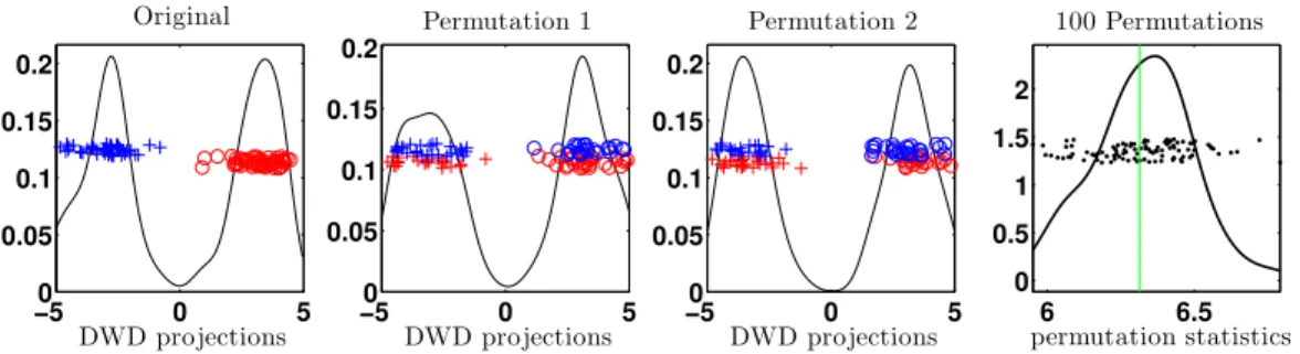
The first panel of Figure 1 shows the one dimensional projection of the data onto the
DWD direction trained on the original class labels. Colors are used to represent original
class membership and are thus constant throughout the first three panels. The projections
are jittered on the y-axis to allow easy visualization. A kernel density estimate of the
projections is plotted in the background (solid black line). We see that the projections in
the first panel of Figure 1 are very well separated despite the fact that the samples arise
from the same underlying distribution. This clear over-fitting artifact common in HDLSS
data is a strong motivation for DiProPerm.
The middle two panels of Figure 1 show projections of the data onto re-trained DWD
directions, each based on a realization of randomly permuted class labels. Symbols are
used to represent permuted class labels and are thus different in the first three panels. We
find the projections here to be well separated with respect to the symbols. Relative to
the second and third panels, the original separation we observed in the first panel is quite
unremarkable, suggesting that the two underlying distribution are not different.
The last panel in Figure 1 confirms this observation. We perform a DiProPerm test
with 100 permutations and display the statistic, chosen here to be the difference of sample
−50 0 5 0.05
0.1 0.15 0.2
Original
DWD projections
−50 0 5
0.05 0.1 0.15 0.2
Permutation 1
DWD projections
−50 0 5
0.05 0.1 0.15 0.2
Permutation 2
DWD projections
6 6.5
0 0.5 1 1.5 2
permutation statistics 100 Permutations
Figure 1: The data are standard 1000-variate Guassian. In the first panel, the DWD
direction is trained on the original class labels, represented by colors (same in all panels).
In the second and third panels, the DWD directions are trained on realizations of randomly
permuted class labels, represented by symbols (different in each panel). The separation
in the first panel is comparable to that in the second and third panels. One hundred
permutation statistics resulting from a DiProPerm test are shown in the last panel which
confirms the separation in the first panel is not significant.
on the unprojected data. We see that based on the DiProPerm test, the null hypothesis of
equal distributions should not be rejected.
1.2 The Hypotheses
Let X1, . . . , Xm and Y1, . . . , Yn be independent random samples of Rd-valued random
vec-tors, d≥1 with distributionsF1 and F2, respectively. We are interested in testing the null
hypothesis of equality of distributions
H0:F1 =F2 versus H1:F1 6=F2 (1)
Letµ(F) denote the mean of a distributionF. Another item of interest is to test the weaker
null hypothesis of equality of means
H0:µ(F1) =µ(F2) versus H1:µ(F1)6=µ(F2) (2)
Note that the multivariate Behrens-Fisher problem concerns testing (2) under normality.
1.3 Overview
The outline for the paper is as follows. A review of related work is presented in Section 2.
In Section 3, two DiProPerm tests are closely examined. HDLSS asymptotics are used to
in Section 4. In Section 5 we perform a Monte Carlo power study comparing DiProPerm
to other methods. Finally in Section 6, DiProPerm is applied to a real microarray dataset.
2
Related work
There is extensive literature on testing equality of distributions for two multivariate
dis-tributions under the classical setting of sample size larger than dimension. For the more
challenging HDLSS setting, several methods have been developed and we discuss two of
them here.
First, there are nearest neighbor tests Bickel and Breiman (1983); Henze (1988); Schilling
(1986) which are based on nearest neighbor coincidences - the number of neighbors around
a data point that belong to the same sample. The null distribution of the test statistic can
be derived parametrically using normal theory or nonparametrically using a permutation
test. A more recent contribution to testing equality of distributions under HDLSS settings
is Szekely and Rizzo’s nonparametric energy test (Szekely and Rizzo, 2004). The energy
test statistic is based on the Euclidean distance between pairs of sample elements. Here
significance is accessed through permutation testing.
The nearest neighbor test and the energy test require calculation of all pairwise distances
between sample elements. The computational complexity of both tests is independent of
dimension, and is thus suitable for the HDLSS setting. In Section 5.1 we perform an
empirical power study comparing DiProPerm to the energy test.
For testing equality of means for two multivariate distributions, the classical Hotelling
T2 test is often used in the setting of sample size larger than dimension. However, the HotellingT2statistic is not computable in HDLSS situations because the covariance matrix
is not of full rank. To address this issue, the methods in (Bai and Saranadasa, 1996),(Chen
and Qin, 2010), and (Srivastava and Du, 2008) replace the covariance matrix in the Hotelling
T2 statistic by a diagonalized version.
Taking a different approach, the method proposed by Lopes et al. projects the high
dimensional data onto a random subspace of low enough dimension so that the traditional
HotellingT2statistic may be used (Lopes et al., 2011). All of these tests have the
disadvan-tage that equal covariances are assumed, which is not a restriction we place on DiProPerm.
In Section 5.2 we perform an empirical power study comparing DiProPerm to the Random
3
The Choice of The Univariate Statistic
Here, we study the difference between two particular choices of the univariate statistic
in Step 2 of DiProPerm. First, let the Mean Difference (MD) direction be the vector
connecting the centroids of each sample. For simplicity, we will use this particular direction
to compare two natural statistics of the projections: 1) the Mean Difference (MD) statistic
— the difference of sample means, and 2) the two-sample t-statistic (t) — difference of
sample means divided by{s1/m+s2/n}1/2 wheres1 ands2 are sample standard deviations
of each class, sized m and nrespectively. Henceforth we specify different DiProPerm tests
by concatenating the direction name and two sample univariate statistic name. Following
this convention, the DiProPerm test that uses the MD direction and the MD statistic will
be referred to as the MD-MD test and the DiProPerm test that uses the MD direction
and the two-sample t statistic as the MD-ttest.
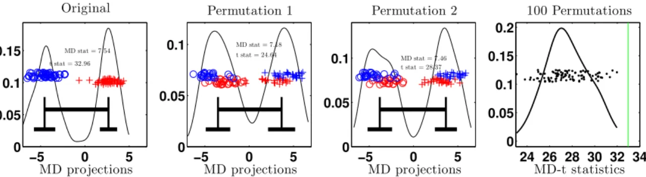
We provide a toy example to contrast the difference between the MD and t statistic.
We draw independent samples, each of size 50, where the first sample arises from the
1000-variate standard Gaussian distribution and the second the 1000-1000-variate distribution with
iid marginal t(5) distributions. Note that the samples arise from different distributions
that have thesame means. Figure 2 shows the one dimensional projection of the data onto
various MD directions and the MD and t statistic applied to these projections.
The lengths of the longer horizontal black bars represent the MD statistics while the
lengths of the shorter horizontal bars represent the sample standard deviations of the
pro-jected data in each permuted group. The MD statistic and two-sample t statistic calculated
on the projected data are displayed towards the top of each panel. We see that the
t-statistic in the first panel is much higher than the permuted t-t-statistics in the second and
third panels. On the other hand, the MD statistic is about the same between the original
and permuted worlds. We confirm this is a systematic pattern by looking at 1000
permuta-tions and calculating the MD-t statistic. The distribution of the permuted MD-t statistics
can be seen in the last panel of Figure 2. We see that the original MD-t statistic,
repre-sented as a vertical line, is among the larger permutation statistics, leading us to reject the
null hypothesis. The distribution of the MD-MD permutation statistics, not shown here,
looks very similar to the last panel of Figure 1, where the original statistic is close to the
middle of the permutation distribution. Thus under this setting the MD-t test rejects the
null while the MD-MD does not.
This apparent inconsistency is due to the fact that the MD and t statistics are actually
−5 0 5 0
0.05 0.1 0.15
Original
MD projections
t stat = 32.96 MD stat = 7.54
−5 0 5 0
0.05 0.1
Permutation 1
MD projections
MD stat = 7.18 t stat = 24.64
−5 0 5 0
0.05 0.1
Permutation 2
MD projections
MD stat = 7.46 t stat = 28.37
24 26 28 30 32 34 0
0.05 0.1 0.15 0.2
MD-t statistics 100 Permutations
Figure 2: The first sample arises from a standard 1000-variate Gaussian distribution and
the second sample arises from the 1000-variate distribution with iid t(5) marginals. In the
first panel, the MD direction is trained on the original class labels, represented by colors.
In subsequent panels, the MD direction is trained on realizations of permuted class labels,
represented by symbols. Note that the MD-MD statistic is similar across the first three
panels while the MD-t statistic is much larger in the first panel. One thousand permutation
MD-t statistics are shown in the last panel. The empirical p-value is small suggesting the
test that uses MD-t would reject the null.
while the latter is testing the strong hypothesis of equality of distributions. In light of this,
each test is correct in its decision. This phenomenon is studied in detail in the next section.
4
Hypothesis Test Validity
In this section, we study the validity of the MD-MD and the MD-t for testing 1) equality
of distributions and 2) equality of means. We work with the MD direction because it is
most amenable to theoretical analysis. Future work will include other directions such as
DWD, SVM, etc. High dimensional geometric representation of SVM and DWD described
in Bolivar-Cime and Marron (2013) could provide the basis for this endeavor.
That both the MD-MD and the MD-t are exact tests for equality of distributions follows
from standard theory on permutation tests. We will discuss how an exact level α test can
Vm,n(Zπ(1), . . . , Zπ(N)) is an exact levelα test. The exactness comes from the fact that the
unconditional distribution and the permutation distribution of the statistic coincide under
the null of equal distributions. It follows that the MD-MD test and the MD-t test, and any
other DiProPerm test, are exact for testing equality of distributions.
The matter of establishing validity for testing equality of means is not as straightforward
on the other hand. In general, permutation tests cannot be expected to be valid for testing
weaker hypotheses such as equality of means. For instance, if the covariances are not the
same, we have to be very careful with our choice of direction and two-sample statistic. The
signal in the covariances may confound our interpretation of tests that are sensitive to both
the signal in the mean and the signal in the variances. This is consistent with our results
which show that under normality and balanced sample sizes, the MD-MD remains valid for
testing equality of means under heterogeneous covariances. On the other hand, the MD-t
is invalid when the covariances are not the same.
4.1 MD-MD
In this section, we establish that the MD-MD test is an exact test for equality of means
under normality and balanced sample sizes. The MD-MD test statistic, Tm,n(Z), is the
mean of the projections of theX’s onto the unit vector in the direction of ¯X−Y¯ minus the
mean of the projections of the Y’s onto the unit vector in the direction of ¯X−Y¯:
Tm,n(Z) =Tm,n(X1, . . . , Xm, Y1, . . . , Yn) (3)
= 1
m
m X
i=1
Xi0 ( ¯X−Y¯)
||X¯ −Y¯|| − 1
n
n X
j=1
Yj0 ( ¯X−Y¯)
||X¯−Y¯|| (4)
=||X¯ −Y¯|| (5)
Theorem 1. Let X1, . . . , Xm be an iid sample from the d-variate Gaussian distribution
N(µX,Σx)and Y1, . . . , Yn be an independent sample drawn iid from the d-variate Gaussian
distribution N(µY,Σy) where ΣX 6= ΣY. Ifm =n then the unconditional distribution and
the permutation distribution of Tm,n(Z) are equal under the null µX =µY.
Proof. UnderµX =µY, ¯X−Y¯ is distributed as
N(0,Σx/m+ Σy/n) (6)
and the permutation distribution of ¯X−Y¯ is
m X
r=0
m r
n r
N m
N
0,(m−r)Σx+rΣy m2 +
rΣx+ (n−r)Σy
n2
If m=n, the expressions in (6) and (7) are the same, in which case the unconditional and
permutation distribution of Tm,n(Z) are also the same.
4.2 MD-t
The MD-t statistic, denoted by Um,n(Z), is the result of applying the unbalanced sample
sizes, unequal variance two-sample t-test statistic (also known as Welch’s t-test (Welch,
1947)) to the projections onto the MD direction. Leta·bdenote the standard dot product
between two vectors inRd. The sample variances of the projected data can be expressed as
s2X˜ = 1
m−1 m X
i=1
[(Xi−X¯)·( ¯X−Y¯)]2
and
s2Y˜ = 1
n−1 n X
i=1
[(Yi−Y¯)·( ¯X−Y¯)]2.
Define Sm,n(Z) =Sm,n(X1, . . . , Xm, Y1, . . . , Yn) =s2X˜/m+s2Y˜/n. The MD-t statistic is
Um,n(Z) =Um,n(X1, . . . , Xm, Y1, . . . , Yn) =Tm,n(Z)2/{Sm,n(Z)}1/2
where Tm,n(Z) is as in Section 4.1. We use the term “projected” rather loosely here since
we have not normalized by||X¯−Y¯||. This is of no actual consequence since the two-sample
t-statistic is scale invariant.
Under equal means the numerator in the MD-t statistic behaves similarly in the
permu-tation world and the original world. However, we will see that the denominator of the MD-t
statistic has very different behavior. We find that the denominator of the MD-t is larger in
the permuted world, as seen in Figure 2. This has the effect of making the unconditional
distribution of the MD-t statistic larger than the permutation distribution.
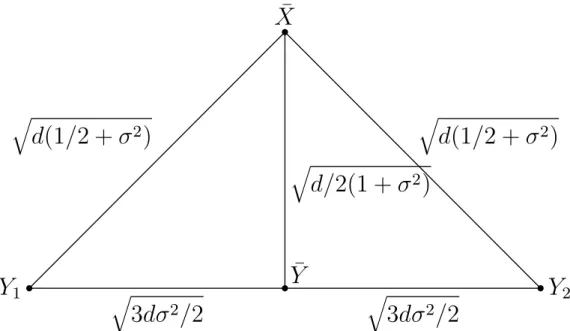
To gain some intuition, consider the following toy HDLSS example. Suppose we observe
X1, X2 ∼ F1 and Y1, Y2 ∼ F2 where F1 = N(0, Id) and F2 = N(0, σ2Id), σ2 6= 1. The
points X1, X2, Y1, Y2 form the vertices of a tetrahedron in three dimensional space. The
two-dimensional plane generated by Y1, Y2 and ¯X is shown in Figure 3. Distances between
elements of interest are calculated using standard HDLSS asymptotics, see Hall et al. (2005)
for examples of this type of calculation. All distances have an additional OP(1) term that
is not shown to avoid clutter. The geometric configuration in Figure 3 has the implication
that s2Y˜ is small. To see this, note the projections of Y1 and Y2 onto the MD direction
¯
X−Y¯ is close to the projection of ¯Y itself. A similar argument can be applied to shows2˜
q
3
dσ
2/
2
q
3
dσ
2/
2
q
d
(1
/
2 +
σ
2)
q
d
(1
/
2 +
σ
2)
q
d/
2(1 +
σ
2)
¯
X
Y
1Y
2¯
Y
Figure 3: Plane generated by Y1, Y2 and ¯X where X1, X2 ∼ F1 = N(0, Id) and Y1, Y2 ∼
F2 =N(0, σ2Id) forσ2 6= 1. Note that the projections ofY1 and Y2 onto ¯X−Y¯ is close to
the projection of ¯Y onto ¯X−Y¯. This has the implication that s2˜
Y will be small.
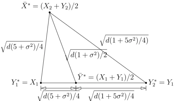
Now let’s look at what happens in the permutation world. Figure 4 shows the
two-dimensional plane generated by the realization of a random permutation where X1∗ =X2,
X2∗ = Y2 and Y1∗ = X1 and Y2∗ = Y1. Notice that the distance between Y1∗ and ¯X∗ is
different than the distance between Y2∗ and ¯X∗. This has the effect of making s2 ˜
Y∗, the
sample variance of the the projections ofY1∗ andY2∗, large. To see this, note the projections of Y1∗ and Y2∗ onto the permuted MD direction are not close to the projection of ¯Y∗. A similar argument can be applied to show s2
˜
X∗, the sample variance of the projections ofX1∗
and X2∗, is large. The derivations for the distances shown in Figures 3 and 4 can be found in the supplement.
The toy example above suggests the denominator of the MD-t statistic is larger in the
permutation world than in the original world. The next result gives us a sense of just how
far apart are the permutation and unconditional distributions of Sm,n(Z).
Theorem 2. LetX1, . . . , Xmbe a sample from the d-variate Gaussian distributionN(µx, σx2Id)
andY1, . . . , Ynbe an independent sample from the d-variate Gaussian distributionN(µy, σ2yId)
where σ2
x6=σy2 are scalars. Under µx=µy, we have 1
dSm,n(Z)
d −→ (σ
2
x
m + σy2
n)
( 1
m−1
σ2
x
mχ
2(m−1) + 1
n−1
σy2 nχ
q
d
(1 + 5
σ
2)
/
4)
q
d
(5 +
σ
2)
/
4
q
d
(1 +
σ
2)
/
2
¯
X
∗= (
X
2+
Y
2)
/
2
Y
1∗=
X
1Y
2∗=
Y
1¯
Y
∗= (
X
1+
Y
1)
/
2
q
d
(5 +
σ
2)
/
4
q
d
(1 + 5
σ
2)
/
4
Figure 4: Plane generated by a particular permutation realization of X1, X2, Y1, and Y2.
Note that the projections of Y1∗ and Y2∗ onto ¯X∗−Y¯∗ is not close to the projection of ¯Y∗
onto ¯X∗−Y¯∗. This has the implication that s2˜
Y∗ may be large.
as d goes to infinity. For the permuted version, we have for some non-zero constantc,
1
d2Sm,n(Zπ)→c in probability.
The results of this theorem are surprising in that the denominator of the MD-t statistic
is actually of different orders in the unconditional and permutation worlds. In particular,
in the unconditional world Sm,n(Z) grows like a random variable times d, while in the
permutation world it grows like a constant times d2.
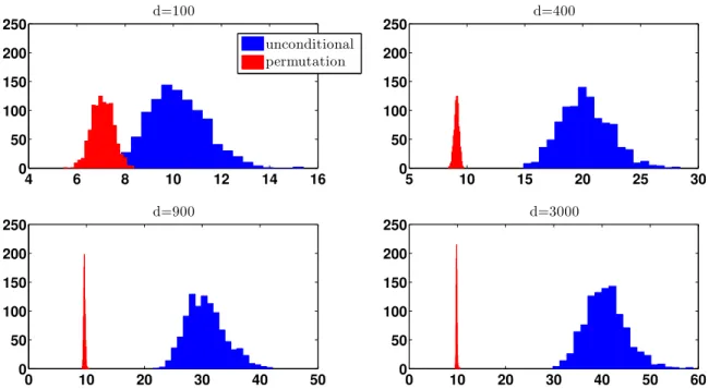
Let us revisit the toy example earlier and see what Theorem 2 can tell us. We make
50 draws from F1 = N(0, Id) and another 50 independent draws from F2 = N(0,100Id).
We show in Figure 5, using 1000 Monte Carlo realizations, the simulated permutation and
unconditional distributions of the MD-t statistic for various dimensions.
Under the conditions in Theorem 2, whenµx=µy, the numerator of the MD-t statistic
is proportional to aχ2(d) variable for both the unconditional and permutation distribution. On the other hand, by the results in Theorem 2 Sm,n(Z) is of the order
√
dand dfor the
unconditional and permuted distributions, respectively. Thus we should expect the MD-t
statistic to be of the order√din the original unconditional world and 1 in the permutation
4 6 8 10 12 14 16 0
50 100 150 200
250 d=100
5 10 15 20 25 30
0 50 100 150 200
250 d=400
0 10 20 30 40 50
0 50 100 150 200
250 d=900
0 10 20 30 40 50 60
0 50 100 150 200
250 d=3000
unconditional permutation
Figure 5: The unconditional and permutation distribution of the MD-t statistic for the
dis-tributions F1 =N(0, Id) and F2 =N(0,100Id). The separation between the unconditional and permutation distribution increases with dimension.
√
dwhile the permutation distribution is not growing with d. As Figure 5 illustrates, the
unconditional distribution quickly separates from the permutation distribution as dimension
increases. Thus it is very important that the MD-t statistic not be used when the goal is
to test for equality of means. On the other hand, this shows the MD-t test has some power
for testing equality of distributions against equal means alternatives.
4.3 Power surfaces
In this section, we study the power of the MD-MD and MD-t for testing equality of means.
In the simulations that follow, we makemdraws fromF1=N(µ1, σ12Id), andnindependent draws from F2 =N(0, Id). We set d= 500 and m =n= 50 for balanced sample sizes and
m= 50, n= 100 for unbalanced. The dimension dand sample sizesm and nare chosen to
reflect a HDLSS setting. The significance level is set at α= 0.05. Power is estimated using
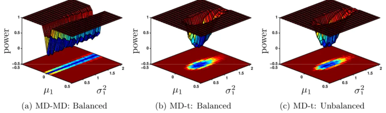
1000 Monte Carlo simulations. Figure 6 displays a 3D surface of power versus µ1 versus
σ2
1, using a color spectrum from cool to warm corresponding to the range 0 to 1. We also
show an image underneath the surface where each pixel corresponds to the point in the 3D
Figure 6a displays the estimated power surface of MD-MD under balanced sample sizes.
By Theorem 1, MD-MD is an exact test for equality of means under balanced sample sizes
and normality. This is consistent with what we see in Figure 6a — when the means are equal
(i.e. µ1 = 0), the power is around α = 0.05, as indicated by the streak at µ1 = 0. When
sample sizes are unbalanced, see Figure 11 in Section B of the Supplement, the MD-MD is
no longer an exact test and may not even be asymptotically valid asd→ ∞. In Section B
of the Supplement, we propose a modification of MD-MD that should be used when sample
sizes are unbalanced.
−0.5 0 0.5 0.5 1 1.5 2 −0.5 0 0.5 1 σ2 1 µ1 p ow er
(a) MD-MD: Balanced
−0.5 0 0.5 0.5 1 1.5 2 −0.5 0 0.5 1 σ2 1 µ1 p ow er
(b) MD-t: Balanced
−0.5 0 0.5 0.5 1 1.5 2 −0.5 0 0.5 1 σ2 1 µ1 p ow er
(c) MD-t: Unbalanced
Figure 6: Power surfaces for testing equality of means of the distributionsF1 =N(µ1, σ21Id) and F2 = N(0, Id). We see that MD-MD attains the correct level under balanced sample sizes. The MD-t test is not valid for testing equality of means regardless of balanced or
unbalanced sample sizes.
Figures 6b and 6c show that under heterogeneous covariances (whenσ2
1 6= 1), the
MD-t MD-tesMD-t of equal means does noMD-t aMD-tMD-tain MD-the correcMD-t level for eiMD-ther balanced or unbalanced
sample sizes. In the immediate region around (µ1, σ12) = (0,1), the power of the MD-t
test is close to α as expected. However as we move away from (µ1, σ12) = (0,1), the power
quickly increases. Thus if we use the MD-t test for equality of means, we will reject too
often. On the other hand this shows that the MD-t test has some power for testing equality
of distributions against alternatives where the means are equal but the distributions are
not.
5
Comparison with Other Methods
In this section we compare DiProPerm to other methods in the simulation contexts described
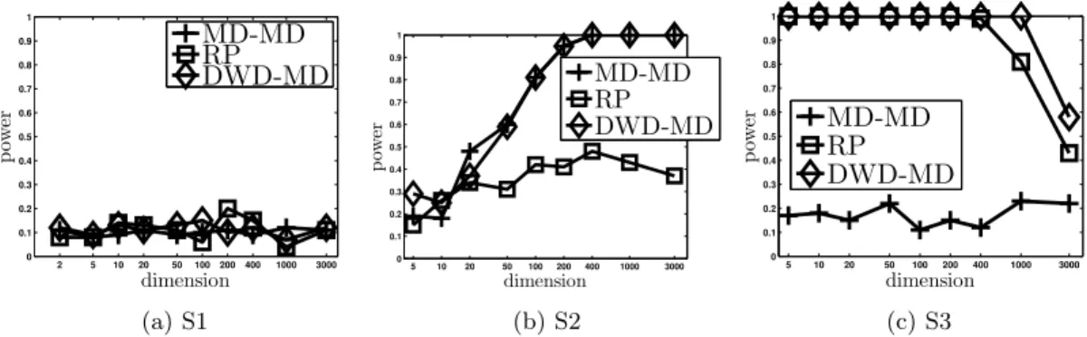
in Table 1. First, for testing equality of distributions, we compare the DiProPerm tests
2004). Next, for testing equality of means, we compare the DiProPerm tests DWD-MD and
MD-MD to the Random Projection test proposed by Lopes, Jacob and Wainwright (Lopes
et al., 2011). Our simulation results show that no test is universally most powerful. As
such, our goal is to learn general lessons about the situations under which each method can
be expected to do well.
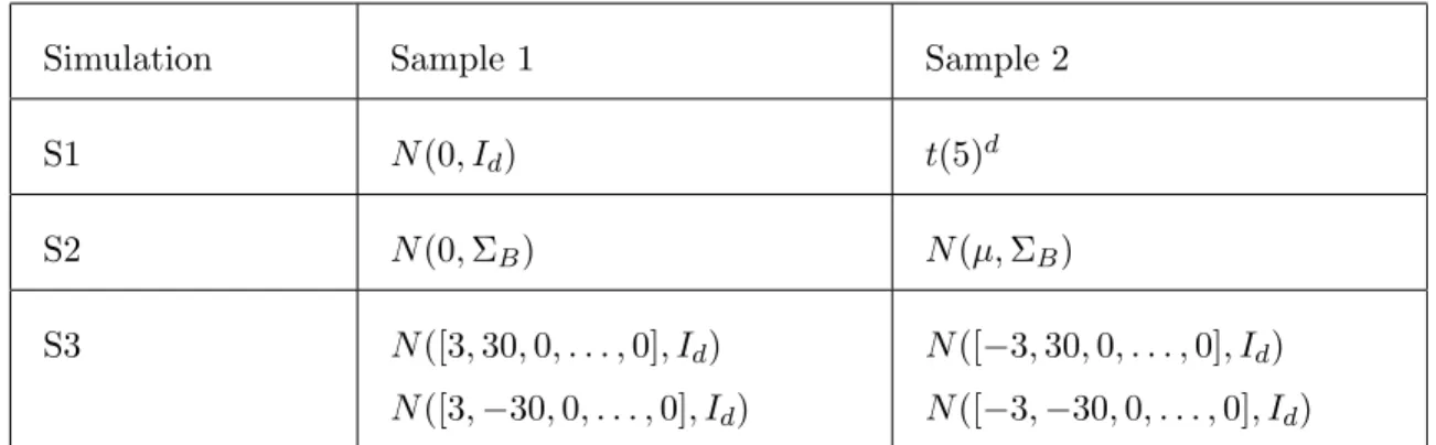
Simulation Sample 1 Sample 2
S1 N(0, Id) t(5)d
S2 N(0,ΣB) N(µ,ΣB)
S3 N([3,30,0, . . . ,0], Id)
N([3,−30,0, . . . ,0], Id)
N([−3,30,0, . . . ,0], Id)
N([−3,−30,0, . . . ,0], Id)
Table 1: Simulation settings. The notation N(µ,Σ) denotes a multivariate Gaussian
dis-tribution with mean µ and covariance Σ. In S1, the notation t(5)d denotes the d-variate
distribution with iid marginal distribution t(5). In S2, the first 25% of the coordinates in
µ are zero and the rest are set to 1/√n. The covariance matrix ΣB has a block structure
(described further in the text). In S3, each distribution is an equally weighted Gaussian
Mixture of the components listed.
Simulation S1 in Table 1 was taken from Szekely and Rizzo. Simulation S2 is a
modifi-cation of a simulation found in Lopes, Jacob, and Wainwright. Following their simulation
setting, we let the covariance matrix ΣB be block-diagonal with identical blocks B ∈R5×5
along the diagonal. The matrix B has diagonal entries equal to 1 and off-diagonal entries
equal to 0.2. The mean vector is set to the zero vector in sample 1. In the second sample,
the mean vector is set to zero in the first 25% of the coordinates and the rest is set to
1/√n. Simulation S3 looks at data arising from equally weighted Gaussian mixtures with
the components listed in Table 1. All DiProPerm tests are implemented using 1000
permu-tations. Power is estimated through 1000 Monte Carlo simulations at 0.1 significance level.
5.1 Equality of distributions
The energy statistic is based on the Euclidean distance between pairs of sample elements.
The two-sample test statistic is
m,n =
mn N
2
mn
m X
i=1
n X
j=1
||Xi−Yj|| − 1
m2
m X
i=1
m X
j=1
||Xi−Xj|| − 1
n2
n X
i=1
n X
j=1
||Yi−Yj||
The first term measures the average distance between the samples and the last two terms
measure the average distance within each sample. The significance of the energy test
statis-tic is assessed using a permutation test. In our implementation of the energy test, we used
1000 permutations.
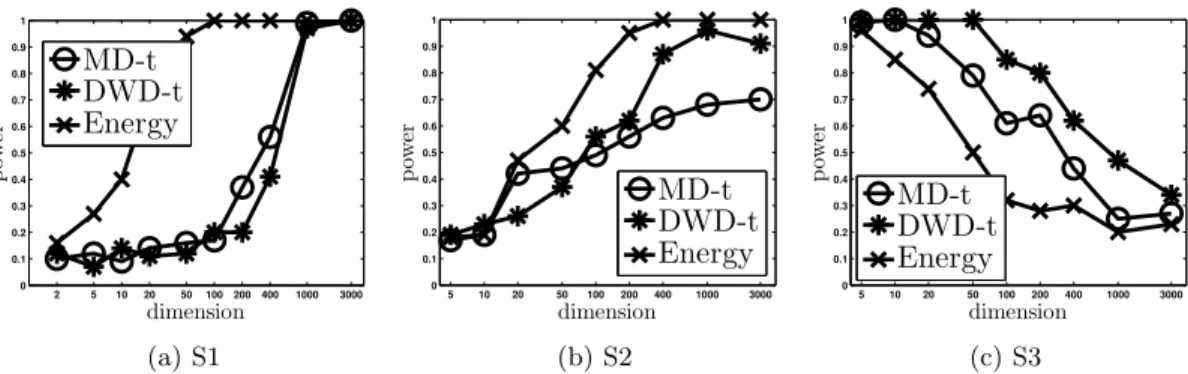
For all simulations in Figure 7, the sample sizes are set to be unbalanced: m= 50, n=
150. Figure 7 compares the power of MD-t, DWD-t, and the energy test for testing equality
of distributions. The first panel shows the result of simulation S1. The standard Gaussian
and t(5)dboth have mean zero but different covariances. Note that the signal in the
covari-ance grows stronger with dimension. In light of this, it is not surprising that the MD-t and
DWD-t do not perform as well as the energy test which is more attuned to variance effects.
However, as the dimension increases all three tests attain full power.
The second panel of Figure 7 shows the results for simulation S2. All three tests perform
well with power increasing to 1 with dimension. Note that the mean effect is along the 45
degree line. The structure of ΣB has the implication that the directions with highest
variation are for some constant c, (c, c, c, c, c,0, . . . ,0), (0,0,0,0,0, c, c, c, c, c,0, . . . ,0), and
etc. Thus the mean effect is further exaggerated by the covariance structure making this a
rather unchallenging setting for all three methods.
The result of simulation S3 is shown in the last panel of Figure 7. Here, both the
DiProPerm DWD-t and MD-t test are seen to be more powerful than the energy test. This
is not surprising since by way of its construction, the energy test can be expected to have
difficulty in separating Gaussian mixture data types. The MD-t has good performance but
DWD-t has the best power because DWD was developed to handle Gaussian mixture data
types.
5.2 Equality of means
In the RP test proposed by Lopes, Jacob and Wainwright, the data is first projected down
to a dimension low enough so that the regular Hotelling T2 statistic may be applied (Lopes
2 5 10 20 50 100200400 1000 3000 0 0.1 0.2 0.3 0.4 0.5 0.6 0.7 0.8 0.9 1 dimension p ow er MD-t DWD-t Energy (a) S1
5 10 20 50 100 200 400 1000 3000 0 0.1 0.2 0.3 0.4 0.5 0.6 0.7 0.8 0.9 1 dimension p ow er MD-t DWD-t Energy (b) S2
5 10 20 50 100 200 400 1000 3000 0 0.1 0.2 0.3 0.4 0.5 0.6 0.7 0.8 0.9 1 dimension p ow er MD-t DWD-t Energy (c) S3
Figure 7: Power comparison of DWD-t, MD-t and the energy test for testing equality of
distributions under the various simulation settings in Table 1.
dimension of the lower dimensional subspace. In our implementation of the RP method, we
follow the authors’ recommendation and set the tuning parameterk=bn/2c. The samples
are assumed to arise from Gaussian distributions with equal covariances. The resulting
statistic then follows an F distribution under the null of equal means. For all simulations
in Figure 8, the sample sizes are set to be balanced: m = 50, n = 50. The standard
multivariate Gaussian and the multivariatet(5)dboth have mean zero, and thus the power
of MD-MD and RP should be around α = 0.1 in simulation S1. The first panel of Figure
8 shows this is indeed the case. Note that if MD-MD or RP were to be used for testing
equality of distributions, neither would have power against alternatives such as in S1.
In simulation S2, the RP method does not perform as well as MD-MD or DWD-MD. This
is perhaps due to the DiProPerm tests being able to pick up the mean effect more efficiently
than the RP method which tries to sense random directions in very high dimensions. Note
that simulation S2 is a setting in which the MD statistic is powerful for either direction
DWD or MD as the mean effect is strong. Re-examining Figure 7, we see that the
DWD-MD is more powerful than the DWD-t and the DWD-MD-DWD-MD more powerful than the DWD-MD-t for
simulation S2. Recall that the covariance structure in S2 amplifies the mean effect. The
DiProPerm tests that use the two-sample t-statistic may have lower power than their MD
counterpart because the standardization in the t-statistic cancels out some of the effect.
In the Gaussian mixture S3 simulation, the DWD-MD and the RP test are both
substan-tially more powerful than the MD-MD test. In this setting, the direction of discrimination
is in the first coordinate direction but the direction of most variation is along the second
coordinate. Not surprisingly, MD-MD has trouble in this setting. The RP test, which uses
direction. DWD-MD is seen to perform slightly better than the RP test. Again, DWD is
designed to work well in discriminating Gaussian mixture data types and this result matches
our expectation.
2 5 10 20 50 100200400 1000 3000 0 0.1 0.2 0.3 0.4 0.5 0.6 0.7 0.8 0.9 1 dimension p ow er MD-MD RP DWD-MD (a) S1
5 10 20 50 100 200 400 1000 3000 0 0.1 0.2 0.3 0.4 0.5 0.6 0.7 0.8 0.9 1 dimension p ow er MD-MD RP DWD-MD (b) S2
5 10 20 50 100 200 400 1000 3000 0 0.1 0.2 0.3 0.4 0.5 0.6 0.7 0.8 0.9 1 dimension p ow er MD-MD RP DWD-MD (c) S3
Figure 8: Power comparison of MD-MD versus the RP method for testing equality of means
under the various simulation settings in Table 1.
6
Application: Microarray data analysis
The first application of DiProPerm to a real dataset can be found in Wichers et al. (2007).
DiProPerm was applied to an HDLSS dataset and used to find a statistically significant
difference between heart rates of rats among different treatment groups. In this section we
will apply DiProPerm to a different kind of HDLSS data — gene expression microarray
data.
Two HDLSS datasets are examined. The first dataset is denoted UNCGEO and the
second UNCUP, following the naming convention of their source which can be found at
http://peroulab.med.unc.edu/. The UNCGEO datasets consists of gene expression data
of 9674 genes measured on 50 breast cancer patients at UNC. The UNCUP dataset looks
at the same set of genes measured on 80 breast cancer patients in another study at UNC.
We performed many different hypotheses of interest within each dataset. We highlight two
particular comparisons here which highlight the main point that formal hypothesis testing
is an important component of visualization in high dimensions.
The UNCGEO patients are divided into standard breast cancer subtypes: 1) Luminal
A versus 2) Luminal B and the UNCUP data into the groups: 1) Luminals (Luminal A
and Luminal B) versus 2) HER and Basal. Luminals have a very different gene expression
signature from HER and Basal. On the other hand, the difference between Luminal A and
between the gene expression in group 1 and group 2. Note that we have a HDLSS setting
here since the number of genes well exceeds the sample sizes in each subgroup.
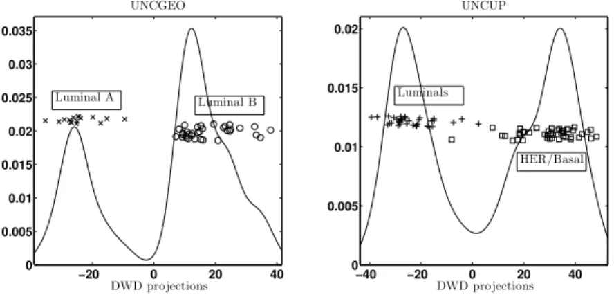
Figure 9 shows the data projected onto DWD directions. The projections in the left
panel do not overlap at all whereas the projections in the right panel have a small amount
of overlap. These projection plots suggest that the separation is better for Luminal A vs.
Luminal B in the UNCGEO dataset than for Luminals vs. HER & Basal in the UNCUP
dataset. However as previously seen in the toy example in Section 1.1, great care is needed
before drawing conclusions of this type.
−20 0 20 40
0 0.005 0.01 0.015 0.02 0.025 0.03 0.035
UNCGEO
DWD projections −40 −20 0 20 40
0 0.005 0.01 0.015 0.02
UNCUP
DWD projections Luminal A Luminal B Luminals
HER/Basal
Figure 9: One dimensional projection plots onto DWD directions for the UNCGEO dataset
and the UNCUP dataset. The separation in the projection plot for the UNCGEO dataset
is more visually pronounced than in the UNCUP dataset. We will rigorously assess this
visual result using DiProPerm.
Figure 10 displays the DiProPerm test results. Each dot represents the test statistic
resulting from a single permutation in the permutation test. We mark the position of the
original univariate t-statistic with a vertical dashed line. The empirical p-values show the
difference in the UNCGEO dataset is not significant while the difference in the UNCUP
dataset is very significant. (We also display the Guasisan fit p-value and Gaussian fit
z-score, two other types of “p-values” described in Section C.3 of the Supplement). This result
on a real world dataset parallels what we saw on the simulated toy dataset in Section 1.1
— what may seem to be a visually striking separation in lower dimensional visualizations
12 14 16 18 20 22 24 26 0
0.02 0.04 0.06 0.08 0.1 0.12 0.14 0.16 0.18 0.2
Statistic UNCGEO: 1000 t−stats from random relabs
t−stat = 17.6799 Emprical pval = 0.31335
Gaussian fit pval = 0.33961
Gaussian fit Z−score = 0.41354
10 12 14 16 18 20 22 0
0.05 0.1 0.15 0.2 0.25 0.3
Statistic UNCUP: 1000 t−stats from random relabs
t−stat = 22.7955 Emprical pval = 0
Gaussian fit pval = 3.667e−012
Gaussian fit Z−score = 6.851
Figure 10: DWD-t test result for the UNCGEO (left) and UNCUP (right) datasets. In the
UNCGEO study (left), the difference between the Luminal A and Luminal B subgroups
is not significant. In the UNCUP study (right), the difference between the Luminals and
HER & Basal subgroups is very significant. This is surprising because the projection plots
in Figure 9 suggest the contrary.
7
Matlab Software
Matlab software for DiProPerm is available athttp://www.unc.edu/~marron/marron_software.html.
Acknowledgements
The work presented in this paper was supported in part by the NSF Graduate Fellowship,
and NIH grant T32 GM067553-05S1.
References
Ahn, J. and Marron, J. S. (2010). The maximal data piling direction for discrimination.
Biometrika, 97(1):254–259.
Bai, Z. and Saranadasa, H. (1996). Effect of high dimension: By an example of a two sample
problem. Statistica Sinica., 6(2):311–329.
Bickel, P. J. and Breiman, L. (1983). Sums of functions of nearest neighbor distances,
moment bounds, limit theorems and a goodness of fit test. The Annals of Probability,
Bolivar-Cime, A. and Marron, J. (2013). Comparison of binary discrimination methods for
high dimension low sample size data. Journal of Multivariate Analysis, 115(0):108 – 121.
Chen, S. X. and Qin, Y.-L. (2010). A two-sample test for high-dimensional data with
applications to gene-set testing. The Annals of Statistics, 38(2):808–835.
Cortes, C. and Vapnik, V. (1995). Support-vector networks. Mach. Learn., 20(3):273–297.
Hall, P., Marron, J. S., and Neeman, A. (2005). Geometric representation of high dimension,
low sample size data. Journal of the Royal Statistical Society Series B, 67(3):427–444.
Hastie, T., Tibshirani, R., and Friedman, J. H. (2003).The Elements of Statistical Learning.
Springer, corrected edition.
Henze, N. (1988). A multivariate two-sample test based on the number of nearest neighbor
type coincidences. The Annals of Statistics, 16(2):pp. 772–783.
Janssen, A. (1997). Studentized permutation tests for non-i.i.d. hypotheses and the
gener-alized behrens-fisher problem. Statistics & Probability Letters, 36(1):9–21.
Jolliffe, I. (2002). Principal Component Analysis. Springer, 2nd edition.
Lopes, M., Jacob, L., and Wainwright, M. J. (2011). A more powerful two-sample test in
high dimensions using random projection. InNIPS, pages 1206–1214.
Mardia, K., Kent, J., and Bibby, J. (1979). Multivariate analysis. Probability and
mathe-matical statistics. Academic Press.
Marron, J., Todd, M. J., and Ahn, J. (2007). Distance-weighted discrimination. Journal of
the American Statistical Association, 102:1267–1271.
Schilling, M. F. (1986). Multivariate two-sample tests based on nearest neighbors. Journal
of the American Statistical Association, 81(395):pp. 799–806.
Srivastava, M. S. and Du, M. (2008). A test for the mean vector with fewer observations
than the dimension. Journal of Multivariate Analysis, 99(3):386–402.
Szekely, G. J. and Rizzo, M. L. (2004). Testing for equal distributions in high dimension.
InterStat, 5.
Welch, B. L. (1947). The Generalization of ‘Student’s’ Problem when Several Different
Wichers, L., Lee, C., Costa, D., Watkinson, W., and Marron, J. (2007). A functional data
analysis approach for evaluating temporal physiologic responses to particulate matter.
A
Proofs
Lemma 1. LetX1, . . . , Xmbe a sample from the d-variate Gaussian distributionN(µx, σx2Id)
andY1, . . . , Ynbe an independent sample from the d-variate Gaussian distributionN(µy, σ2yId)
where σ2
x 6= σ2y. Let X˜k = Xk0( ¯X −Y¯). Let X˜1:k−1 be the sample mean of X˜1, . . .X˜k−1.
Under µx =µy, we have, for k= 2, . . . , m
d−1/2(( ˜X
k−X˜1:k−1))
{k−k1σ2
x(σ2x/m+σ2y/n)}1/2 d
−→ N(0,1) as d→ ∞.
Similarly we have
d−1/2(( ˜Y
k−Y˜1:k−1))
{ k
k−1σ2y(σx2/m+σ2y/n)}1/2 d
−→ N(0,1) as d→ ∞
k= 2, . . . , n.
Proof. We can write ˜Xk−X˜1:k−1 as a sum of products
˜
Xk−X˜1:k−1=
d X
p=1
(Xk−X¯1:k−1)(p)( ¯X−Y¯)(p) (8)
whereX(p) simply refers to thep-th component in the d-dimensional vectorX. The
expec-tation of the summands in (8) is zero:
E(Xk−X¯1:k−1)(p)( ¯X−Y¯)(p)=E(Xk(p)X¯(p))−E( ¯X1:(pk)−1X¯(p))
−E(Xk(p)Y¯(p)) +E( ¯X(p)
1:k−1Y¯(p))
= 0
Next we look at the variance of the summands. Recall for Gaussian data, zero covariance
is equivalent to independence. We know the covariance between (Xk −X¯1:k−1)(p) and
( ¯X−Y¯)(p) is zero since the expectation of the latter is zero and the expectation of the
product was shown above to be zero as well. Thus each summand in (8) is the product of
two independent variables. The variance of a product of independent variables (see ?? for
a derivation), U and V, is
(EU)2V ar(V) + (EV)2V ar(U) +V ar(U)V ar(V). (9) Thus we have
V ar(Xk−X¯1:k−1)(p)( ¯X−Y¯)(p)=V ar(Xk−X¯1:k−1)(p)V ar( ¯X−Y¯)(p)
= k
k−1σ
2
By the Central Limit Theorem, we have
d1/2(1
d( ˜Xk−X˜1:k−1)) { k
k−1σx2(σx2/m+σ2y/n)}1/2 d
−→ N(0,1) asd→ ∞
Lemma 2. LetX1, . . . , Xmbe a sample from the d-variate Gaussian distributionN(µx, σx2Id)
andY1, . . . , Ynbe an independent sample from the d-variate Gaussian distributionN(µy, σ2yId)
where σ2x 6= σ2y. Let π be a permutation of {1, . . . , N = m+n}. Let Z¯π = ( ¯Zπ(1:m) −
¯
Zπ(m+1:N)) be the MD direction trained on the permuted labels determined by π. We have for i= 1, . . . , m,
E((Zπ(i)−Zπ(1:m))(k)Z¯(k)
π )
is non-zero. Similarly, for i=m+ 1, . . . , N, we have
E((Zπ(i)−Zπ(m+1:N))(k)Z¯(k)
π )
is non-zero.
Proof. We prove the first statement. The second can be shown in a similar fashion. Let
P(n, k) denote the number of kpermutations of n, i.e.
P(n, k) =n·(n−1)·(n−2)· · ·(n−k+ 1)
We have fori= 1, . . . , mand k= 1, . . . , d,
E((Zπ(i)−Zπ(1:m))(k)Z¯(k)
π ) =E((Zπ(i)−Z¯π(1:m))(k)( ¯Zπ(1:m)−Z¯π(m+1:N))(k))
=EZπ(k(i))Z¯π(k(1:)m)−EZπ(k()i)Z¯π(k()m+1:N)−E( ¯Zπ(k(1:)m))2+EZ¯π(k(1:)m)Z¯π(k()m+1:N)
= (EZ
(k)
π(i))2
m +
m m−1µ
2−µ2−E( ¯Z(k)
π(1:m))2+µ2
= var(Z
(k)
π(i)) +µ2
m +
m m−1µ
2−(var( ¯Z(k)
π(1:m)) +µ 2)
= var(Z
(k)
π(i))
m −var( ¯Z
(k)
π(1:m))
= m
N{ σx2 m −
1
m2
1
w1
mX−1
r=0
P(m−1, r)P(n, m−r)[rσx2+ (m−r)σy2]}
+ n
N{ σ2y
m −
1
m2
1
w2
n−1 X
r=0
where w1 and w2 are the weights
w1 :=
mX−1
r=0
P(m−1, r)P(n, m−r) and w2:=
n−1 X
r=0
P(n−1, r)P(m, m−r)
Thus if σx2 6=σy2, we have E((Zπ(i)−Zπ(1:m))(k)Z¯(
k)
π ) is nonzero.
Lemma 3. Let Z1, Z2 be two random variables in Rd such that Z1(k)Z
(k)
2 are i.i.d. for
k= 1, . . . , d and E(Z1(k)Z2(k)) exists and is finite. Then
1
d2(Z1·Z2)
2→[E(Z(k) 1 Z
(k)
2 )]2 in probability
Proof. By the Law of Large Numbers, we have
1
d(Z1·Z2)→E(Z
(k) 1 Z
(k)
2 ) in probability.
By Continuous Mapping Theorem, we have
1
d2(Z1·Z2)
2 →[E(Z(k) 1 Z
(k)
2 )]2 in probability.
Now we have all the necessary ingredients to prove Theorem 2 in Section 4.2.
Proof of Theorem 2. To prove the first part of Theorem 2, we decomposes2X˜ and s2Y˜ into a sum of independent variables. Let ˜Xk−1 be the sample mean of the firstk−1 projections
˜
X1, . . .X˜k−1. We will write s2X˜ in a recursive fashion. Define s 2
1 = 0. We will use the
following recursive formula to define s2
k fork= 2, . . . , m
(k−1)s2k = (k−2)s2k−1+k−1
k ( ˜Xk−X˜k−1)
2 (10)
Sinces2
k−1 is independent of ( ˜Xk−X˜k−1)2, this recursive viewpoint allows us to decompose
s2X˜ =s2m into a sum of independent terms. Using the result in Lemma 1 and the second-order Delta method, we have
1
d( ˜Xk−X˜1:k−1)2 k
k−1σx2(σ2x/m+σy2/n) d
−→χ2(1) asd→ ∞ (11)
Inputting expression (11) into the recursion defined in (10) and exploiting the independence
of the individual terms in s2X˜, we get 1 ds 2 ˜ X d −→ 1
m−1σ
2
x(
σ2x m +
σ2
y
n)χ
Similarly, we can show for the sample of projections ˜Y1, . . . ,Y˜n, 1 ds 2 ˜ Y d −→ 1
n−1σ
2
y(
σ2
x
m + σ2y
n)χ
2(n−1) asd→ ∞
Thus we have
1
dSm,n(Z) =
1
d s2X˜
m + s2Y˜
n
!
d
−→ 1
m−1
σx2 m(
σ2x m +
σy2 n)χ
2(m−1) + 1
n−1
σ2y n(
σ2x m +
σy2 n)χ
2(n−1)
For the second part in Theorem 2, we expand the sample variance of the projected
values in the permuted group as follows:
s2Z˜
π(1:m) = 1
m−1 m X
i=1
( ˜Zπ(i)−Z˜π(1:m))2
= 1
m−1 m X
i=1
((Zπ(i)−Zπ(1:m))·( ¯Zπ(1:m)−Z¯π(m+1:N)))2
Lemma 2 showsE(Zπ(i)−Z¯π(1:m))(k)( ¯Zπ(1:m)−Z¯π(m+1:N))(k)is nonzero. Now apply Lemma
3 withZ1= (Zπ(i)−Zπ(1:m)) andZ2= ( ¯Zπ(1:m)−Z¯π(m+1:N)) to see that d12s2Z˜
π(1:m)
converges
in probability to a nonzero constant. A similar argument can be applied to s2Z˜
π(m+1:N). Combining these results, it immediately follows that d12Sm,n(Zπ) converges in probability to a nonzero constant.
B
MD-scaled MD
We established in Section 4.1 that under certain conditions, the MD-MD test is valid when
sample sizes are balanced. Under these same conditions, MD-MD is no longer a valid test
however when sample sizes are unbalanced. Here we propose a modification of MD-MD,
called MD-scaled MD, that is asymptotically valid, asm, n→ ∞ for fixedd, for equality of
means when covariances are unequal and sample sizes are unbalanced.
We have chosen the classical asymptotic regime here to take advantage of the following
results. Janssen proved the permutation test for equality of means based on the studentized
statistic,
m1/2( ¯X−Y¯)/{s2x+m
ns
2
wheres2x and s2y are the standard unbiased estimators ofσx2 andσ2y, is asymptotically valid as m, n → ∞ for the univariate case (Janssen, 1997). Janssen’s result easily extends to
the multivariate case if we assume a spherical covariance structure. Let X1, . . . , Xm be a sample from a d-variate distribution with mean and covariance (µX, σx2Id) andY1, . . . , Ynbe an independent sample with mean and covariance (µY, σy2Id). We propose the MD-scaled MD DiProPerm test whereby the MD direction is used in Step 1 of DiProPerm and a scaled
MD statistic as in Equation (12) is used in Step 2. The MD-scaled MD statistic is
Tm,n(Z)/{s2x/m+s2y/n}1/2 (13) whereTm,n(Z) is as in Section 4.1. The asymptotic validity of the MD-scaled MD statistic
(as m, n → ∞) follows immediately from Janssen’s result. Note that normality is not an
assumption here.
−0.5 0
0.5 0.5
1 1.5
2 −0.5
0 0.5 1
σ2
1
µ1
p
ow
er
(a) MD-MD: Unbalanced
−0.5 0
0.5 0.5
1 1.5
2 −0.5
0 0.5 1
σ2
1
µ1
p
ow
er
(b) MD-scaled MD: Unbalanced
Figure 11: Power surface of the MD-MD and the MD-scaled MD for testing equality of
means for distributions F1 = N(µ1, σ12Id) and F2 = N(0, Id). When sample sizes are
unbalanced, the MD-scaled MD test attains the correct level while the MD-MD does not.
We study the empirical power of the MD-MD and MD-scaled MD for testing equality
of means when sample sizes are unbalanced. We set m = 50, n = 100 and makem draws
from F1=N(µ1, σ21Id) and ndraws from F2 =N(0, Id) for d= 500. The sample sizes and
dimension are chosen to reflect a HDLSS setting. The significance level is set at α= 0.05.
Power is estimated using 1000 Monte Carlo simulations and displayed using a color spectrum
from cool to warm, corresponding to the range 0 to 1.
Figure 11, as in the figures in Section 4.3, displays the simulated power surface of
MD-MD and MD-MD-scaled MD-MD. We see that when sample sizes are unbalanced and covariances
simulated power study also suggests that the asymptotics for the MD-scaled MD test is in
effect for relatively small sample sizes and a much larger dimension.
C
Additional Implementation Options
C.1 Direction
The following binary linear classifiers are among many possible choices for the direction
vector used in Step 1 of DiProPerm and all are implemented in the DiProPerm software:
1. The Mean Difference method is a simple binary linear classifier, also called the centroid
method (Hastie et al., 2003), where points are assigned to the class whose centroid
is closest. The normal vector to the separating hyperplane is the unit vector in the
direction of the line segment connecting the centroids of each class, ( ¯X−Y¯).
2. Fisher Linear Discrimination (FLD) was an early binary linear classification method,
see Chapter 11 of Mardia et al. (1979) for an introduction. FLD seeks a separation
that maximizes the between sum-of-squares of the two classes while minimizing the
within sum-of-squares of each class. The normal vector to the separating hyperplane
is the unit vector in the direction of W−1( ¯X−Y¯)0 whereW is the d×dmatrix
W = m X
i=1
(Xi−X¯)(Xi−X¯)0+ n X
j=1
(Yj−Y¯)(Yj−Y¯)0
3. Support Vector Machine (SVM) is a popular binary linear classification method that
minimizes training error while maximizing the margin between the two classes. See
Hastie et al. (2003) for a good introduction.
4. Distance Weighted Discrimination (DWD) is a binary linear classifier similar to SVM
except each data point has some weight in the final classifier (Marron et al., 2007).
DWD better avoids the data piling problem exhibited by SVM in high dimensions.
5. Maximal Data Piling (MDP) is a binary linear classifier such that the projections
of the data points from each class onto its normal direction vector have two distinct
values (Ahn and Marron, 2010).
Notice that we have not included any PCA directions on this list. This is because PCA is
tailored to find directions that show maximal variation, which is different from our
disadvantage to using PCA as the direction in step 1 of DiProPerm is that the
univari-ate two-sample test statistic calculunivari-ated in step 2 of DiProPerm would be invariant under
relabelings.
C.2 Projection and univariate statistic
In the second step of DiProPerm, we project the data onto the direction in step one and
compute a univariate two-sample statistic on the projected values. Large values of the test
statistic indicate departure from the null hypothesis. The following univariate two-sample
statistics are among many reasonable choices for the DiProPerm procedure and all are
implemented in the DiProPerm software.
1. Two Sample t statistic
2. Difference of sample means
3. Difference of sample means scaled, as in Equation (13)
4. Difference of sample medians
5. Difference of sample medians, divided by the median absolute deviation.
6. Area Under the Curve (AUC), from Receiver Operating Characteristic (ROC) curve
7. Paired sampling t-statistic
It is of interest to note that the classical Hotelling T2 statistic is a special case of the general DiProPerm framework. The FLD direction vector and the difference of sample
means combination gives the statistic ( ¯X−Y¯)W−1( ¯X−Y¯)0. This is in fact the Hotelling
T2 test statistic scaled by a factor of 1
n−2n1nn2. To see this, recall the HotellingT
2 statistic
is
T2 = n1n2
n ( ¯X−Y¯)S
−1
u ( ¯X−Y¯)0
where
Su = Pm
i=1(Xi−X¯)(Xi−X¯)0+Pnj=1(Yj−Y¯)(Yj−Y¯)0
n−2 =
W n−2
The MD-FLD statistic is n−12 n n1n2T
C.3 Permutation
In the final step of DiProPerm, an approximate permutation test is conducted to assess the
significance of the test statistic in step two. Our permutation test is approximate because
we perform a large number of random rearrangements of the labels on the observed data
points, rather than all possible rearrangements. There are three kinds of indicators we
commonly use and all are implemented in the DiProPerm software:
1. Empirical p-value: this is calculated as the proportion of the rearrangement test
statis-tics that exceed the original test statistic. The empiricalp-value has the disadvantage
of often being zero. We may wish to compare two separations to see which is more
significant. This motivates the next quantity.
2. Gaussian fit p-value: we fit a Gaussian distribution to the permutation test statistics
and based on this calculate the percentage of rearrangement test statistics that
ex-ceed the original test statistic. (The term p-value is used loosely here). We do this
not because we believe the permutation statistics are actually Gaussian, but because
this provides a basis on which we can compare two DiProPerm results. In certain
settings where the Gaussian fit p-value may suffer from round-off error, we use the
next quantity as an alternative.
3. z-score: we fit a Gaussian distribution to the permutation test statistics and
calcu-late the corresponding z-score of the original test statistic with respect to the fitted
distribution.
When interpreting the results of DiProPerm tests, it is generally useful to print all three
indicators. When it is non-zero, the empirical p-value is the most interpretable. When it
is zero we next look to the Gaussian fit p-value. Finally if the Gaussian fit p-value suffers
from round-off error, the z-score is preferable.
D
HDLSS calculations
Let X ∼ N(0, σ2xId) and Y ∼ N(0, σy2Id). We will study the asymptotic behavior of the distance between X andY. We have simply by definition
Then by the Central Limit Theorem,
√
d ||X−Y||
2/(σ2
x+σ2y) √
2d −
1 √ 2
!
→N(0,1)
asd→ ∞. Applying the Delta Method, we get
√
d
||X−Y|| 21/4q(σ2
x+σy2)d − 1
21/4
=OP(1)
and thus
||X−Y||=q(σ2
![Crystal structure of a binuclear nickel(II) complex constructed of 1H imidazo[4,5 f][1,10]phenanthroline and doubly deprotonated benzene 1,3,5 tricarboxylic acid](data:image/gif;base64,R0lGODlhAQABAIAAAP///wAAACH5BAEAAAAALAAAAAABAAEAAAICRAEAOw==)