The use of Dielectric Absorption as a Method for Characterizing Dielectric Materials in Capacitors

The use of Dielectric Absorption as a Method for Characterizing Dielectric Materials in

Capacitors

Devin K. Hubbard

A thesis submitted to the faculty of the University of North Carolina at Chapel Hill in

partial fulfillment of the requirements for the degree of Master of Science in the

Department of Biomedical Engineering.

Chapel Hill

2010

Approved by:

Robert G. Dennis, PhD.

Mark Tommerdahl, PhD.

ii

ii

iii

iii

ABSTRACT

DEVIN K. HUBBARD: The use of Dielectric Absorption as a Method for Quantifying

and Qualifying Dielectric Materials in Capacitors.

(Under the direction of Robert G. Dennis, Ph.D.)

Dielectric absorption (soakage) is a phenomenon wherein the stored electric field

within the dielectric of a capacitor will cause the plates of that capacitor to recharge

despite having been fully discharged. Recently Cosmin Iorga proposed a mathematical

model describing dielectric absorption as an infinite sum of decaying exponentials

. We

have expanded on the definition put forth by Iorga and have proposed a model for two

capacitors arranged in parallel. We examine the effect of electrical short time (ts), charge

voltage (Vc), capacitance (C), and dielectric material on maximum absorption signal and

the average time constant of the absorption signal (t68%). While our results are consistent

with those of Iorga, we did observe some divergent behavior for ts > 10 seconds. Our

examination suggests the possibility of using dielectric absorption as a method for sensor

applications to be used in addition to current analytical techniques for characterizing

iv

iv

TABLE OF CONTENTS

List of Tables………...v

List of Figures………vi

Background and Introduction……….1

Definitions and Derivations………4

Materials and Methods………... 8

Results………....11

Discussion………..16

Future Research……….19

Appendices………...22

v

v

LIST OF TABLES

Table

1.

Absorption Response Summary for 10 µF X7R Ceramic Capacitor………...13

vi

vi

LIST OF FIGURES

Figure

1.

Circuit diagram of two capacitors in parallel prior to

being voltage clamped and after being voltage clamped………..8

2.

Comparison of dielectric absorption curves for different dielectrics………...12

3.

Plot of V

vs. ln(t

) for 10 µF X7R Ceramic Capacitor………13

4.

Histogram comparing average t68% of different dielectrics………..14

5.

Plot of t

vs. ln(t

) for a 10 µF X7R Ceramic Capacitor………...15

6.

Plots comparing averaged signals from two

independently charged 10 uF capacitors to the signal

Background and Introduction:

Dielectric absorption, also referred to as soakage or dielectric relaxation, is a

non-linear, non-ideal effect in capacitors wherein electric field stored on the dielectric

material results in a gradual recharging of the capacitor some time after the capacitor has

been shorted or fully discharged

. In a capacitor, current scientific theory suggests that

the dielectric material acts to set up an electric field that opposes the electric field that is

placed between the two plates of a capacitor. As a result, the dielectric in effect ―cancels‖

the external field to some extent, resulting in a net increase in the amount of charge that

can be built up on a capacitor plates. By definition, capacitor dielectric materials must be

insulators to prevent charge from leaking from one side of a capacitor to another

(self-discharge). As a direct consequence of exhibiting suitable electrical insulating ability,

dielectrics tend to be poor conductors of charge within their structure and typically

disperse charge on their surface. Charge redistribution on and in a dielectric is much

slower than in good conductors resulting in a slower change in field condition. If a

capacitor is not completely discharged for a sufficient length of time, the electric field set

up in the dielectric material can pull charge back on to the plates of the capacitor once the

Ohmic load or short circuit condition is removed, resulting in what is most often an

undesirable recharging of the capacitor. Since the ability of each material to redistribute

charge depends on its bulk and surface properties, it follows that every dielectric material

2

2

According to Iorga, the dielectric absorption current onto a capacitor can be

modeled by an infinite sum of decaying exponential currents according to:

(1)

Where the resulting voltage on the capacitor is described by:

(2)

In this method of modeling dielectric absorption, the electric field set up in the dielectric

is described as being manifest in ―compartments,‖ each having its own unique decay rate

(

). The return (absorption) current onto the capacitor is a function of the initial current

in each compartment (

), the length of time that the capacitor is shorted (tsc), and the

length of time (t, which we will refer to as read time t

) that has elapsed since the

shorting period. The dielectric absorption voltage is derived from the return current and is

a function of the capacitance (C); the initial voltage applied to the capacitor, which is

designated as the charge voltage (Vc); the voltage achieved at the end of the short-circuit

discharge of the capacitor, which is designated as the short voltage (Vs); and the internal

impedance of each compartment (R

). Unfortunately in the Iorga model, there is no way

to determine the number of compartments for any given capacitor and therefore one may

only estimate the actual functions that are described. Model equations of the type (1) and

(2) are classically ill conditioned

because fitting them is difficult without knowing

the number of compartments prior to fitting. Iorga put forth a successive subtraction

method that uses asymptotic estimations to successively remove the slowest

compartments (i.e. those which have the largest time constant) from the natural logarithm

3

3

iterations due to successive noise amplification which causes instabilities in the

estimation of asymptotes. Holmstrom et al. point out that when using iterative methods

(which Holmstrom calls graphical methods), if one does a series of Taylor expansions

and logarithmic transformations that one will see clearly that, any component

characterized by a small amplitude and large time constant will be distorted by a large

factor

.

Other methods for fitting such equations have been used widely in atmospheric

sciences to model radiative transmission

. More sophisticated methods for modeling

sums of exponential decays typically make use of inverse-Laplace transforms or a

derivative of non-linear least squares regression (NLLR)

. Literature has reported poor

success of transform methods in general—particularly the inverse Laplace transform

.

Least squares methods offer more promising fits than iterative methods because they

attempt to fit the entire curve at once rather than just find an asymptote—making them

less sensitive to noise and allowing up to four or five iterations to be made before the

method begins to fail. However, an estimation of the number of compartments must be

made prior to actually beginning a NLLR method. Furthermore, initial values must be

given to NLLR methods in order for any convergence to occur. Even with aptly chosen

initial conditions, convergence is not guaranteed, and special constraints must be made to

prevent negative and imaginary coefficients. However, the problem that complicates any

least-squares method is the problem of finding the global minimum of the least-squares

fit. Since the problem is so ill conditioned, there is no way of absolutely ensuring

convergence of the model to the global minimum error. Warren Wiscombe published

4

4

an iterative method of adding and removing terms followed by a non-linear least-squares

regression method to deduce the global minimum solution to a sum of decaying

exponentials—his method reports the ability to accurately model (0.01% to 0.001% error)

as many as 8 compartments on known functions of decaying exponentials

.

Holmstrom presents several other methods for exponential sum fitting, but points

out that it is imperative to have good methods for choosing starting values (he suggests

using geometric methods which he presents). Holmstrom also points out that in solving

the sum of exponentials problem, one is faced with the challenge that a simple method

will give fast results, but poor resolution—while more accurate methods tend to require

more computing time and power. Hence qualifying exponential sum terms is a

challenging endeavor and we approach this problem by describing simple characteristics

of the curve derived from the data in an attempt to show that there is a relationship

between dielectric material and dielectric absorption characteristics.

Definitions and Derivations:

We have decided to use five metrics to describe dielectric absorption in different

materials: dielectric memory (ξ), maximum recharge voltage (Vmax), the first time at

which voltage reaches 68% of the maximum recorded value (V

), the length of time it

takes to reach 68% of the maximum voltage (t68%, or average time constant), and the

leakage (V

–or the difference between the V

and the final absorption voltage, V

).

Each of these metrics is monitored for different charging and discharging patterns. The

adjustable parameters used were the shorting time (ts), charging time (ts), the reading time

(t

), the charge voltage (V

), number of charge/discharge cycles (n), and dielectric

5

5

We define the dielectric memory as the difference between subsequent Vmax

values between charge cycles:

Dielectric Memory (ξ) ≡ Vmax(n) – Vmax(n-1)

(3)

Dielectric memory describes the propensity of the dielectric material to

―remember‖ previous charging cycles. While Vmax describes the severity to which a

dielectric will cause charge to return on to the capacitor in question. We define V68% as:

V

= V(t

) = (0.68)*(V

)

(4)

We use the V68% and the t68% as a metric to describe the rate at which charge

soaking occurs. Finally we define the leakage of a capacitor as:

VL= Vmax – Vf

(5)

Which describes the propensity of poor dielectrics (such as paper in oil) to conduct

charge, therefore contributing to a slow self-discharge of the capacitor which would

manifest itself as a slowly decreasing voltage on the capacitor after it has been charged

and the voltage/current source removed.

An explicit equation for Vmax can be found by taking the limit of equation 2 as

the read time goes to infinity:

Vmax =

(6)

Which for V

= 0:

Vmax =

(7)

From which one can then determine the t68% by substituting V = 0.68*Vmax into equation

6

6

(8)

Which, for a one compartment system collapses to provide an expression for the time

constant for the major contributing compartment (τm

):

(9)

Thus, the t68% can be derived from the weighted average of the decay functions of

the absorption voltage.

According to equation 2, the absorption signal can be thought of as

compartmentalized. Additionally, the model is derived from the assumption that each

soakage compartment is in parallel with the next—it is also assumed that no current

passes between compartments and that the absorption signal does not affect itself (which

implies linear superposition in capacitance). We seek to extend the definition of Iorga to

apply to more general situations wherein a capacitor is in parallel with a second, but with

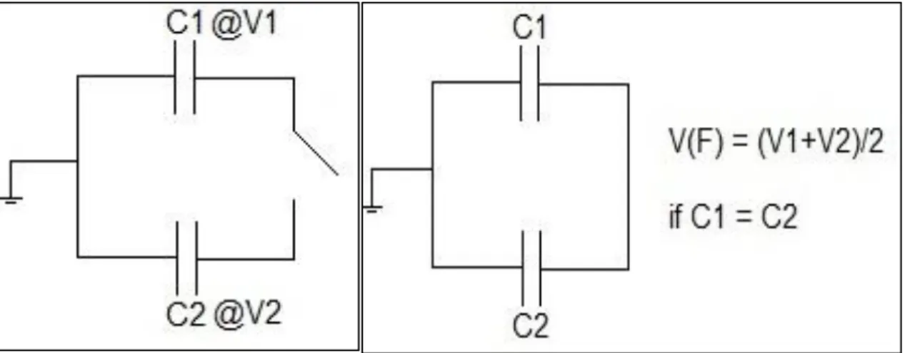
differing dielectric material. One can extend Iorga‘s definition by first considering two

capacitors with charge energy stored in them that will manifest itself in the form of

electrical potentials V1 and V2 for capacitors C1 and C2. If the capacitors are initially

separated by a switch then their respective initial voltages are V

and V

. When the

switch is thrown, the two capacitors are voltage clamped and the final voltage on each

capacitor rises according to the total charge in the system (Figure 1):

q1 = C1V1

(10)

and,

q2 = C2V2

(11)

7

7

Q = q1 + q2 = C1V1 + C2V2

(12)

But since the capacitors are voltage clamped when the switch is thrown

Q = Vf (C1 + C2)

(13)

Where V

is the final voltage across the capacitors. Thus,

C1V1 + C2V2 = Vf(C1 + C2)

(14)

Or,

Vf =

(15)

In order to apply equation 15 to a system of parallel capacitors one must imagine that

after a capacitor is charged and then discharged, there is a certain amount of energy still

set up in the internal electric field within the dielectric. Since the electric field in a

dielectric material is set up as a bulk polarization of the molecules, the rate at which the

field decays in the absence of an external electrical field is typically slower than rate at

which the external electrical field can be removed. As a result, when a capacitor is

shorted briefly so as to rapidly drive the external field to ground, the internal field on the

dielectric does not immediately decay. The remaining internal field in the dielectric

induces a potential on the plates of the capacitor once the Ohmic load or short condition

is released. The effect of the induced potential by the decaying internal electric field of

the dielectric is termed dielectric absorption (or soakage). Assuming that the plates of the

capacitor at the instant after the short is released, start at a potential difference of 0 Volts,

then one can see that all of the energy that will cause dielectric absorption is contained

within the internal electric field of the dielectric. Thus, one can imagine that as the

capacitors recharge, because they are voltage clamped, the charge will distribute itself in

8

8

to the decay rate of the particular dielectric. If one assumes that there is minimal

influence on the absorption signal by the induced external field, then the argument can be

made that the total absorption VT at time ti seen for two parallel capacitors will be

identical to the capacitance-weighted average of their individual signals at time t

when

not in parallel, or:

VT(ti) =

(16)

For the case when C1 = C2 the total voltage at any given time becomes the average of the

two absorption signals:

V

(t

)=

(17)

The capacitance for each capacitor is defined as:

C =

(18)

Where ε is the dielectric constant, A and d are the area and separation distance of the

capacitor plates respectively. Combining the formula for capacitance with equation 17

and inserting equation 2 for V

(t

) and V

(t

):

VT(ti) =

(19)

Where n(ti) =

. Thus, the total

voltage at any given time should be proportional to the capacitance weighted average of

the individual absorption signals. If the capacitance of the two capacitors in question is

equal, then the total voltage is simply an average of the two individual signals—and since

9

9

dielectric constant), the total absorption voltage depends on the dielectric properties of

the individual capacitors.

Figure 1: (Left) Two capacitors, C1 and C2 charged to voltages V1 and V2 are separated by a switch.

(Right) When the switch is thrown, the total charge of the system redistributes to satisfy the fact that the capacitors are now voltage clamped.

Materials and Methods:

Hardware:

Charging and data collection hardware was designed in-house by Avery Cashion

and Robert Dennis; details of the circuit are given elsewhere

. Data was collected at

83.33 Hz using the specially designed hardware with a USB interface to a computer

running a visual basic (VB) graphical user interface (GUI) designed by Avery Cashion.

The VB GUI provided the ability to adjust charging time (t

), shorting time (t

), reading

time (tr), charging voltage (Vc), and number of charge/discharge cycles (n).

In order to examine dielectric absorption we examined effect of each of the

following variables on the five metrics described above:

Effect of Electrical Short time (t

):

In order to examine the effects of the short time on capacitors, a series of tests

10

10

time was examined for each dielectric at 2.5 V, 5 V and 10 V charging signals. In each

case the capacitors were charged for 65 seconds and were then read for 65 seconds to

ensure complete signal acquisition. A test series consisted of 10 cycles of charging,

shorting and reading to ensure sufficient data for averaging. Since the capacitors were

discharged through some nominal resistance (internal to the circuitry), it was important to

examine the effects of short times that are as close to the RC time constant of the circuit

as possible—1 ms was well above the RC time constant for the largest capacitor used

(220 µF Electrolytic).

Reading time (t

):

In order to ensure adequate signal acquisition, all experiments used a minimum of

45 seconds recording time and at most 65 seconds of recording time.

Effect of Dielectric Material (ε):

Since we propose that the dielectric material has a large effect on the shape and

properties of the dielectric absorption signal, we have explored several different dielectric

materials. Common Y5V and X7R ceramic (0.47 µF and 10 µF supplied by Digikey

Corporation, Thief River Falls, MN), aluminum electrolytic (220 µF and 10 µF supplied

by Digikey Corporation, Thief River Falls, MN), and paper-in oil (PIO) capacitors

(generously donated by Dietolf Ramm of the Durham FM Association) were used in our

experiments.

Effect of Charge Voltage (V

):

Observing the Iorga description of dielectric absorption, it is clear that the initial

11

11

series of charge voltages was devised to examine the effect of charge voltage on

dielectric absorption. Charge voltage was examined at 10 volts, 5 volts and 2.5 volts.

Effect of Parallel Capacitance:

Since the Iorga model treats compartments as electronically parallel units we have

explored the idea of placing two different dielectric materials in parallel to examine the

difference between the native absorption signals of each of the dielectrics and the signal

when placed in parallel. Herein we explored a 10 µF ceramic capacitor in parallel with a

10 µF electrolytic capacitor.

Effect of Capacitance:

According to the Iorga model, as the capacitance increases the dielectric

absorption should be scaled by the inverse of the capacitance. We compared Vmax

between a 0.47 µF and 10 µF ceramic capacitor as well as between a 10 µF and 220 µF

aluminum electrolytic capacitor.

Analysis Software:

The data acquired were reshaped and filtered using a custom MatLab script

(Appendix C). The data were filtered using a rank-3 median filter in software prior to

being analyzed. Software algorithms were employed to determine the maximum voltage

reached as well as the t68%.

Results:

General Observations:

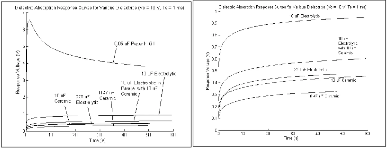
A representative absorption curve from each of the capacitors examined is

provided in figure 2. Each curve was generated for a charging voltage of 10V and a short

12

12

appeared to systematically decrease with each additional cycle—an observation that will

require further study. Furthermore, we also observe that the 10 µF electrolytic capacitor

has a larger absorption signal than the 220 µF electrolytic capacitor of the same variety—

however it is interesting to note that the 0.47 µF ceramic capacitor appears to have a

smaller absorption signal than the 10 µF ceramic capacitor in figure 1.

Figure 2: Left: Plot of the absorption curves over a 65 second interval for each of the capacitors examined. Short time was 1 ms, charge voltage was 10 volts. Right: A plot of the absorption curves over a 65 second

interval for each capacitor examined excluding the paper-in-oil capacitor. Short time was 1 ms, charge voltage was 10V.

Vmax:

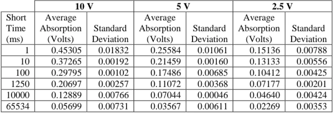
The effect of short time, dielectric and charging voltage on the maximum

dielectric absorption signal was examined and representative data is presented in table 1

(additional data are summarized in appendix A). Average absorption signal was

calculated from 10—charge/short/read cycles. According to equation 2, the voltage at any

given point should be proportional to an infinite sum of curves containing a decaying

exponential in short time—thus a semi-logarithmic plot of maximum absorption voltage

vs. short time is generated in figure 3 for the representative 10 µF ceramic capacitor

(additional plots found in appendix B). Our general observation was that the PIO

13

13

ceramic capacitors which had a maximum recharge voltage in the range of 0.2 V to 0.6 V

when charged to 10 V and shorted for 1 ms. It is also important to note that the PIO

capacitor displayed leakage for brief short times and higher charge voltages while no

leakage was observed in ceramic or electrolytic capacitors.

Table 1: Absorption response summary for a 10 µF ceramic capacitor (Digikey Corporation, Thief River Falls, MN) for charge voltages of 10, 5 and 2.5 volts. All signals and standard deviations are an average of 10 charge/short/read cycles and are in volts.

10 V 5 V 2.5 V

Short Time (ms) Average Absorption (Volts) Standard Deviation Average Absorption (Volts) Standard Deviation Average Absorption (Volts) Standard Deviation 1 0.45305 0.01832 0.25584 0.01061 0.15136 0.00788 10 0.37265 0.00192 0.21459 0.00160 0.13133 0.00556 100 0.29795 0.00102 0.17486 0.00685 0.10412 0.00425 1250 0.20697 0.00257 0.11072 0.00368 0.07177 0.00201 10000 0.12889 0.00766 0.07044 0.00046 0.04640 0.00424 65534 0.05699 0.00731 0.03567 0.00611 0.02269 0.00353

Figure 3: Plot of Vmax after 65 seconds vs. natural logarithm of short time for a 10 µF ceramic capacitor for 10V, 5 V and 2.5 V charge voltage for 65 seconds. The plot displays near-linearity which can be

explained by the relationship between absorption signal and short time in equation 2.

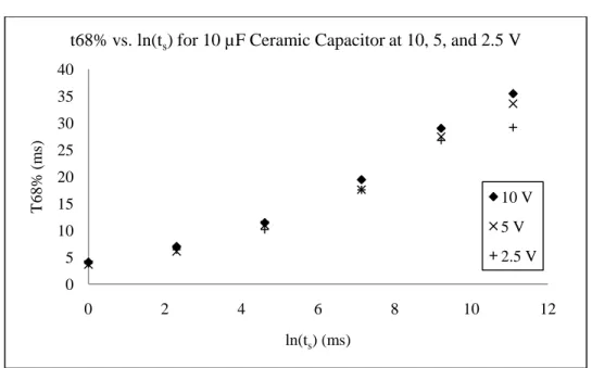
t

:

The effect of short time, dielectric and charge voltage on the average time

constant of the dielectric absorption response was examined and displayed in Table 2. It

V_max= -0.0356ln(t_s)+ 0.4564 R² = 0.9992

V_max= -0.0203ln(t_s)+ 0.2599 R² = 0.9968

V_max = -0.0118ln(t_s)+ 0.1556 R² = 0.9969

0 0.05 0.1 0.15 0.2 0.25 0.3 0.35 0.4 0.45 0.5

0 2 4 6 8 10 12

Vm ax ( Vo lts )

ln(t_s) (ms)

Vmax vs. ln(t

) for 10 µF Ceramic Capacitor at 10, 5 and 2.5 V

14

14

should be noted that the 68% recovery time should be independent of charge voltage and

that the observed data seem to follow that trend. It should also be noted that additional

data are summarized in appendix B and that for most dielectrics t68% seems to be

independent of charging voltage, provided the short time is less than 10 seconds. For the

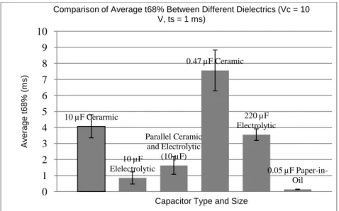
case of a charging voltage of 10 V and a short time of 1 ms, the respective average t68%

for PIO, 0.47 µF ceramic, 10 µF ceramic, 10 µF electrolytic, 220 µF electrolytic, and 10

µF ceramic with 10 µF electrolytic in parallel are (figure 4): 0.1370 + 0.0106 ms, 7.5568

+ 1.2697 ms, 4.0680 + 0.7160 ms, 0.8496 + 0.3785 ms, 3.5500 + 0.3634 ms, and 1.6284

+ 0.5562 ms.

Figure 4: Representative histogram comparing the average t68% of each of the capacitors tested herein for a

charge voltage of 10 V and a short time of 1 ms.

10 µF Cerarmic

10 µF Elelectrolytic

Parallel Ceramic and Electrolytic

(10 µF)

0.47 µF Ceramic

220 µF Electrolytic

0.05 µF Paper-in-Oil 0 1 2 3 4 5 6 7 8 9 10 A v e ra g e t 6 8 % ( m s )

Capacitor Type and Size

15

15

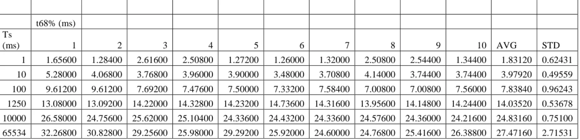
Table 2: Average ‗time constant‘ (t68%) for a 10 µF X7R ceramic capacitor (Digikey Corporation, Thief

River Falls, MN) for charge voltages of 10, 5 and 2.5 volts. All signals and standard deviations were derived from an average of 10 charge/short/read cycles.

10 V

5 V

2.5 V

Short

Time

(ms)

t68%

(ms)

Standard

Deviation

t68%

(ms)

Standard

Deviation

t68%

(ms)

Standard

Deviation

1

4.06800

0.71682

3.64920

0.71158

3.82200

0.92398

10

6.98280

0.19493

6.09360

0.15857

6.39240

0.75508

100

11.41200

0.10076

10.94760

0.77116

10.15080

0.75807

1250

19.42920

0.20392

17.56440

1.15609

17.52960

0.49786

10000

28.99080

0.39918

27.44640

0.56636

26.75160

1.00387

65534

35.44440

1.41154

33.56400

1.09436

29.15467

2.65081

Figure 5: Plot of t68% vs. natural logarithm of ts for a 10 µF X7R capacitor (Digikey Corporation, Thief

River Falls, MN) for charge voltages of 10, 5 and 2.5 volts.

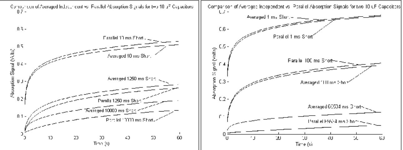
Parallel Capacitors:

Figure 4 shows a comparison of the absorption signal from the two 10 µF

capacitors placed in parallel to the average of the signals from each capacitor separately.

Our observations indicate that as the short time increases, the disparity between the

averaged signals and the parallel signal deviate from each other more drastically.

0 5 10 15 20 25 30 35 40

0 2 4 6 8 10 12

T 6 8 % ( m s)

ln(t_s) (ms)

t68% vs. ln(t

) for 10 µF Ceramic Capacitor at 10, 5, and 2.5 V

10 V

5 V

16

16

Figure 6: Plots comparing the average of two independently charged 10 µF capacitors (one ceramic, and one electrolytic) to the signal collected from the same two 10 µF capacitors while in parallel. The absorption signal is in volts and the time is tracked in seconds.

Discussion:

The majority of our observations are quite consistent with the mathematical

description of dielectric absorption provided by Iorga. We have noted some interesting

behaviours that, to our knowledge, have not been described in the literature. Robert Pease

described compensation circuitry for dielectric absorption and in his data it appears as if

the soakage signal becomes increasingly small with each new charge/discharge cycle,

however no comments are made regarding this particular occurrence

. We consistently

observed that the first cycle, in particular, of nearly every soakage series resulted in a

larger signal than the subsequent cycles. While our observation is not discretely

explained by the mathematics of Iorga or those derived herein, it is quite possible that the

effect being observed may be a result of the previous charge series or the influence of the

dielectric signal on itself—however the explanation remains unclear and further

investigation of this peculiar effect is warranted.

Iorga‘s equations suggest that the absorption voltage should be inversely

17

17

to be the case for the two electrolytic capacitors examined, we did find that the ceramic

capacitors examined did not behave according to the expected behavior. It is possible that

this disparity might be attributed to differing temperature coefficients (Y5V vs. X7R) and

material composition. Further experiments should be carried out in order to determine the

more general effect of capacitance on dielectric absorption response.

According the Iorga‘s model, the maximum absorption voltage should be related

to short time by an infinite sum of decaying exponentials. As a result the maximum

observed recharge voltage should display linearity when plotted against the logarithm of

short time. Our observations agree with the linearity observed for the X7R 10 µF ceramic

capacitor suggesting that the capacitor conforms to Iorga‘s model. The degree of linearity

of the semi-logarithmic plot in time is indicative of an exponential relationship between

absorption signal and short time. Any deviation from linearity is suggestive of a more

complex relationship between short time and recharge voltage. Our data indicates that for

some capacitors, at larger short times the behaviour of the semi-log plot in time deviates

from linear—suggesting that perhaps there is an additional factor unaccounted for in the

Iorga model. It is worth noting that if one were to plot the logarithm of Vmax with respect

to time, the degree of linearity of this semi-logarithmic plot should be an indicator of how

many compartments one might require to model the dielectric response of a particular

capacitor. The more linear the semi-log plot in V

, the fewer compartments that are

required to describe the response—which is to say that the response of a linear semi-log

plot in Vmax suggests a simple exponential relationship between short time and voltage, or

18

18

increases, so also does the number of compartments required to describe the capacitor by

Iorga‘s model.

Leakage in the capacitors was only observed significantly and consistently in the

PIO capacitor. While a systematic examination of this leakage behaviour is not conducted

herein, it is important to note that the amount of leakage and the shape of the absorption

curves appear to vary in both short time, as well as charge voltage. Further examination

of leakage in capacitors may prove useful in sensor applications for dielectric absorption.

According to equation 8, t68% is completely independent of charging voltage and

capacitance, but is dependent on short time and compartment properties (compartment

internal impedance Rj and compartment time constant τj). As a result, the t68% offers a

quantitative description of the compartment properties within a dielectric that is

independent of the dielectric constant. This independence from dielectric constant and

capacitance does not preclude variance in t68% between different capacitors because it

remains dependent upon the unique properties R

and τ

which are specific to each

dielectric. Presumably Rj and τj are also specific to the relative proportion and

distribution of compounds within a dielectric, however further investigation will be

required in order to draw conclusions regarding the relationship between material

distribution in dielectric and absorption response.

Parallel capacitors examined herein presented varying results. For brief short

times (typically less than 10 seconds), the absorption curve of the parallel capacitors

seemed to be closely modeled by the average of the absorption signals of the individual

capacitors under the same charging and shorting conditions. It is also interesting to note

19

19

signal, and in other cases the averaged signal was less. Additional experiments should be

run while varying capacitance and dielectric material in order to better understand the

phenomenon. For cases where the short time was larger than 1 second, the averaged

signal was always larger than the parallel signal. There are several possible reasons for

the trend observed for large short times. It is possible that the equations derived

describing the parallel signal need to be modified to account for an increase in overall

capacitance of the system equal to the sum of the parallel capacitances. For two

capacitors in parallel, it is also possible that the self-influence the dielectric absorption

has on itself is attenuated (or possibly amplified) significantly enough to cause significant

differences between the averaged independent signals and the parallel signal. It is also

worth noting that Iorga‘s model assumes that no current flows between compartments—

an assumption that cannot be made in the case of parallel capacitors as current must flow

between capacitors (which are treated as large compartments in this model) in order to

maintain the clamped voltage condition. A more thorough examination of parallel

capacitors should be conducted in order to aid in sensor circuitry development since the

capacitance of the circuit could influence the obtained signal.

Our observations herein suggest that further experimentation should be conducted

to completely describe the absorption responses of common capacitors. Our data suggests

that different dielectric materials have distinguishable absorption signals. Further

mathematical descriptions will be required in order to determine as much useable

information about a signal as possible if the possibility of a sensor application is to be

realized. The assumptions inherent in the current mathematical description of absorption

20

20

which the short time is significantly longer than compartments with small time constants

and low internal resistances, the way in which the absorption signal affects itself is likely

to change significantly from those obtained under conditions of small short time. Since

the current mathematical tools for fitting sums of decaying exponentials are poorly suited

for fitting the absorption response curves, a possibility for identifying different dielectric

materials based on absorption signal may be more appropriately solved by

implementation of a support vector machine. Our data generally support the possibility of

using dielectric absorption as a method for characterizing dielectric materials. Specific

potential applications of the principles outlined here include devices for capacitor quality

control, assessment of lipid-base biofuels, and assessment of biomass feedstock for

production of alternative fuels. Future research will better indicate the strengths and

weaknesses inherent in using dielectric absorption in sensor applications.

Future Research:

Future research will focus on examining more capacitors to better understand the

effect of dielectric material and capacitance on the absorption signal. Different parallel

setups will be used to better understand how to model parallel capacitors of differing

composition and size. It would also be interesting to examine the leakage behaviour in

capacitors and how it relates to absorption signal. Research is currently under way using

a custom capacitor with variable dielectric and capacitance to examine the effect of

varying dielectric concentration using a liquid, lipid-based dielectric material. Finally, in

an effort to better predict the signal of an unknown mixture of materials, the use of

support vector machines will be implemented to ascertain the possibility of creating a

21

21

including geology, industrial quality control and process monitoring, biomedical and

electrical engineering. When coupled with methods such as dielectric, UV-visual, nuclear

magnetic resonance spectroscopy and mass spectrometry, dielectric absorption could help

provide additional information about internal dielectric behaviours of materials.

Conclusion:

While our observations are consistent with those of Iorga, we did observe several

aberrations that need further exploration. The purpose of this examination was to

determine the viability of dielectric absorption in sensing techniques. While additional

research will be required to determine better metrics, our preliminary results indicate that

t68% is a potentially useful metric when describing dielectric absorption that is

independent of dielectric constant. Our examination of parallel capacitors has shed some

light on the question as to whether the possibility of differentiating two materials in a

capacitor is possible. Our results agree with the proposed model for two parallel

capacitors under conditions of small short time; however, further examination will be

required to characterize the response of parallel capacitors after long short times (ts > 10

s). Our treatment of the system is greatly simplified—many assumptions are inherent in

the equations that are currently used to describe dielectric absorption. In order to properly

characterize dielectric materials, it will be imperative to develop methods for analyzing

an entire absorption response curve. Support vector machines offer a promising

alternative to previously attempted modeling schemes for characterizing the infinite sums

of decaying exponentials that make up the absorption signals

. Future research will focus

22

22

based on support vector machine interpretation in an effort to aid in the global

23

23

24

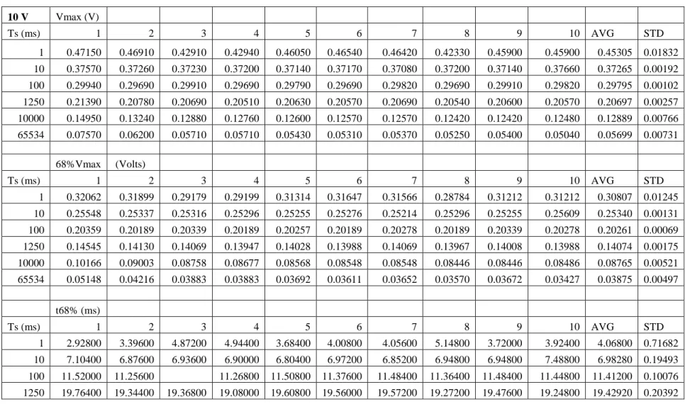
Table 3: Summary of Vmax data for the 10 µF Ceramic capacitor. Short time (ts) is in ms, Vmax is in volts, averages and standard deviations are listed at the

right. Each row represents 10 charge/short/cycles and are numbered 1-10. This table represents data taken for 10V, 5 V and 2.5V charging voltages. Within each charging voltage the Vmax vs ts data is shown, followed by 68%Vmax vs ts, followed by a table of t68% vs. ts. All times are expressed in milliseconds. Blank cells

represent unusable data.

10 V Vmax (V)

Ts (ms) 1 2 3 4 5 6 7 8 9 10 AVG STD

1 0.47150 0.46910 0.42910 0.42940 0.46050 0.46540 0.46420 0.42330 0.45900 0.45900 0.45305 0.01832

10 0.37570 0.37260 0.37230 0.37200 0.37140 0.37170 0.37080 0.37200 0.37140 0.37660 0.37265 0.00192

100 0.29940 0.29690 0.29910 0.29690 0.29790 0.29690 0.29820 0.29690 0.29910 0.29820 0.29795 0.00102

1250 0.21390 0.20780 0.20690 0.20510 0.20630 0.20570 0.20690 0.20540 0.20600 0.20570 0.20697 0.00257

10000 0.14950 0.13240 0.12880 0.12760 0.12600 0.12570 0.12570 0.12420 0.12420 0.12480 0.12889 0.00766

65534 0.07570 0.06200 0.05710 0.05710 0.05430 0.05310 0.05370 0.05250 0.05400 0.05040 0.05699 0.00731

68%Vmax (Volts)

Ts (ms) 1 2 3 4 5 6 7 8 9 10 AVG STD

1 0.32062 0.31899 0.29179 0.29199 0.31314 0.31647 0.31566 0.28784 0.31212 0.31212 0.30807 0.01245

10 0.25548 0.25337 0.25316 0.25296 0.25255 0.25276 0.25214 0.25296 0.25255 0.25609 0.25340 0.00131

100 0.20359 0.20189 0.20339 0.20189 0.20257 0.20189 0.20278 0.20189 0.20339 0.20278 0.20261 0.00069

1250 0.14545 0.14130 0.14069 0.13947 0.14028 0.13988 0.14069 0.13967 0.14008 0.13988 0.14074 0.00175

10000 0.10166 0.09003 0.08758 0.08677 0.08568 0.08548 0.08548 0.08446 0.08446 0.08486 0.08765 0.00521

65534 0.05148 0.04216 0.03883 0.03883 0.03692 0.03611 0.03652 0.03570 0.03672 0.03427 0.03875 0.00497

t68% (ms)

Ts (ms) 1 2 3 4 5 6 7 8 9 10 AVG STD

1 2.92800 3.39600 4.87200 4.94400 3.68400 4.00800 4.05600 5.14800 3.72000 3.92400 4.06800 0.71682

10 7.10400 6.87600 6.93600 6.90000 6.80400 6.97200 6.85200 6.94800 6.94800 7.48800 6.98280 0.19493

100 11.52000 11.25600 11.26800 11.50800 11.37600 11.48400 11.36400 11.48400 11.44800 11.41200 0.10076

25

10000 29.53200 29.08800 29.29200 29.40000 29.23200 28.68000 28.70400 28.94400 28.82400 28.21200 28.99080 0.39918

65534 36.62400 37.10400 35.65200 36.42000 35.84400 34.74000 35.08800 35.52000 31.98000 35.47200 35.44440 1.41154

5 V Vmax (V)

Ts (ms) 1 2 3 4 5 6 7 8 9 10 AVG STD

1 0.25090 0.26430 0.26280 0.23710 0.26280 0.26000 0.23680 0.26250 0.26060 0.26060 0.25584 0.01061

10 0.21760 0.21640 0.21610 0.21360 0.21330 0.21450 0.21390 0.21450 0.21270 0.21330 0.21459 0.00160

100 0.19290 0.17760 0.17700 0.17360 0.17090 0.17210 0.17270 0.17030 0.17090 0.17060 0.17486 0.00685

1250 0.10250 0.10740 0.10960 0.11600 0.11020 0.11140 0.11230 0.11230 0.11260 0.11290 0.11072 0.00368

10000 0.07050 0.07020 0.07050 0.06960 0.07080 0.07020 0.07050 0.07020 0.07140 0.07050 0.07044 0.00046

65534 0.05100 0.04030 0.03750 0.03450 0.03330 0.03330 0.03230 0.03140 0.03110 0.03200 0.03567 0.00611

68%Vmax (Volts)

Ts (ms) 1 2 3 4 5 6 7 8 9 10 AVG STD

1 0.17061 0.17972 0.17870 0.16123 0.17870 0.17680 0.16102 0.17850 0.17721 0.17721 0.17397 0.00722

10 0.14797 0.14715 0.14695 0.14525 0.14504 0.14586 0.14545 0.14586 0.14464 0.14504 0.14592 0.00109

100 0.13117 0.12077 0.12036 0.11805 0.11621 0.11703 0.11744 0.11580 0.11621 0.11601 0.11890 0.00465

1250 0.06970 0.07303 0.07453 0.07888 0.07494 0.07575 0.07636 0.07636 0.07657 0.07677 0.07529 0.00250

10000 0.04794 0.04774 0.04794 0.04733 0.04814 0.04774 0.04794 0.04774 0.04855 0.04794 0.04790 0.00032

65534 0.03468 0.02740 0.02550 0.02346 0.02264 0.02264 0.02196 0.02135 0.02115 0.02176 0.02426 0.00416

t68% (ms)

Ts (ms) 1 2 3 4 5 6 7 8 9 10 AVG STD

1 5.29200 3.28800 3.27600 4.23600 3.34800 3.15600 4.23600 3.31200 3.15600 3.19200 3.64920 0.71158

10 6.09600 6.24000 6.21600 5.94000 5.89200 6.25200 6.09600 6.28800 5.84400 6.07200 6.09360 0.15857

100 12.86400 11.20800 11.44800 10.95600 10.30800 10.66800 10.74000 10.32000 10.44000 10.52400 10.94760 0.77116

1250 15.88800 16.76400 17.14800 20.36400 17.02800 17.35200 17.96400 17.70000 17.78400 17.65200 17.56440 1.15609

26

65534 35.16000 34.34400 34.30800 33.73200 33.10800 34.54800 31.44000 33.34800 32.49600 33.15600 33.56400 1.09436

2.5 V Vmax (V)

Ts (ms) 1 2 3 4 5 6 7 8 9 10 AVG STD

1 0.15810 0.16110 0.14620 0.15780 0.15590 0.15530 0.15500 0.14100 0.14280 0.14040 0.15136 0.00788

10 0.14590 0.13400 0.13210 0.13030 0.13030 0.12700 0.12970 0.12880 0.12820 0.12700 0.13133 0.00556

100 0.11440 0.10770 0.10530 0.10350 0.10380 0.10250 0.10130 0.10100 0.10130 0.10040 0.10412 0.00425

1250 0.07690 0.07290 0.07200 0.07170 0.07170 0.07080 0.06990 0.07050 0.07050 0.07080 0.07177 0.00201

10000 0.05710 0.04910 0.04760 0.04640 0.04550 0.04390 0.04360 0.04390 0.04330 0.04360 0.04640 0.00424

65534 0.03110 0.02530 0.02230 0.02200 0.02170 0.02080 0.02080 0.02010 0.02010 0.02269 0.00353

68%Vmax (Volts)

Ts (ms) 1 2 3 4 5 6 7 8 9 10 AVG STD

1 0.10751 0.10955 0.09942 0.10730 0.10601 0.10560 0.10540 0.09588 0.09710 0.09547 0.10292 0.00536

10 0.09921 0.09112 0.08983 0.08860 0.08860 0.08636 0.08820 0.08758 0.08718 0.08636 0.08930 0.00378

100 0.07779 0.07324 0.07160 0.07038 0.07058 0.06970 0.06888 0.06868 0.06888 0.06827 0.07080 0.00289

1250 0.05229 0.04957 0.04896 0.04876 0.04876 0.04814 0.04753 0.04794 0.04794 0.04814 0.04880 0.00136

10000 0.03883 0.03339 0.03237 0.03155 0.03094 0.02985 0.02965 0.02985 0.02944 0.02965 0.03155 0.00288

65534 0.02115 0.01720 0.01516 0.01496 0.01476 0.01414 0.01414 0.01367 0.01367 0.01543 0.00240

t68% (ms)

Ts (ms) 1 2 3 4 5 6 7 8 9 10 AVG STD

1 5.95200 3.63600 4.46400 3.25200 3.06000 2.97600 2.89200 4.03200 4.22400 3.73200 3.82200 0.92398

10 8.18400 6.82800 6.55200 6.16800 6.52800 5.40000 6.36000 6.06000 6.14400 5.70000 6.39240 0.75508

100 11.38800 11.42400 10.54800 9.81600 10.20000 10.04400 9.30000 9.79200 9.62400 9.37200 10.15080 0.75807

1250 17.90400 18.18000 18.08400 18.12000 17.00400 17.14800 16.89600 17.50800 17.26800 17.18400 17.52960 0.49786

10000 28.15200 27.27600 26.82000 28.36800 27.34800 25.59600 25.99200 26.35200 25.80000 25.81200 26.75160 1.00387

27

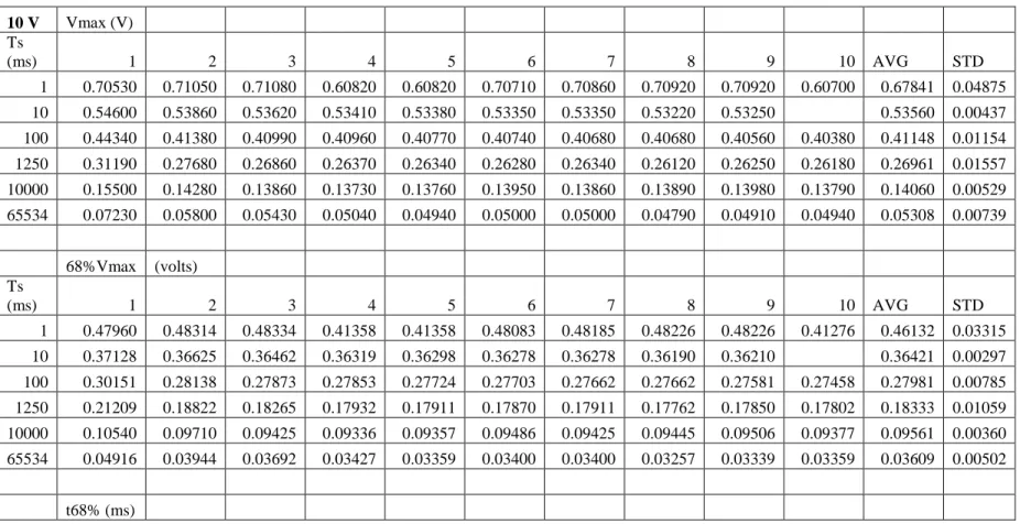
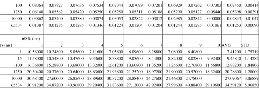
Table 4: Summary of Vmax data for the 10 µF X7R ceramic capacitor with 10 µF electrolytic capacitor in parallel. Short time (ts) is in ms, Vmax is in volts,

averages and standard deviations are listed at the right. Each row represents 10 charge/short/cycles and are numbered 1-10. This table represents data taken for 10V, 5 V and 2.5V charging voltages. Within each charging voltage the Vmax vs ts data is shown, followed by 68%Vmax vs ts, followed by a table of t68% vs. ts. All

times are expressed in milliseconds. Blank cells represent unusable data.

10 V Vmax (V)

Ts

(ms) 1 2 3 4 5 6 7 8 9 10 AVG STD

1 0.70530 0.71050 0.71080 0.60820 0.60820 0.70710 0.70860 0.70920 0.70920 0.60700 0.67841 0.04875

10 0.54600 0.53860 0.53620 0.53410 0.53380 0.53350 0.53350 0.53220 0.53250 0.53560 0.00437

100 0.44340 0.41380 0.40990 0.40960 0.40770 0.40740 0.40680 0.40680 0.40560 0.40380 0.41148 0.01154

1250 0.31190 0.27680 0.26860 0.26370 0.26340 0.26280 0.26340 0.26120 0.26250 0.26180 0.26961 0.01557

10000 0.15500 0.14280 0.13860 0.13730 0.13760 0.13950 0.13860 0.13890 0.13980 0.13790 0.14060 0.00529

65534 0.07230 0.05800 0.05430 0.05040 0.04940 0.05000 0.05000 0.04790 0.04910 0.04940 0.05308 0.00739

68%Vmax (volts)

Ts

(ms) 1 2 3 4 5 6 7 8 9 10 AVG STD

1 0.47960 0.48314 0.48334 0.41358 0.41358 0.48083 0.48185 0.48226 0.48226 0.41276 0.46132 0.03315

10 0.37128 0.36625 0.36462 0.36319 0.36298 0.36278 0.36278 0.36190 0.36210 0.36421 0.00297

100 0.30151 0.28138 0.27873 0.27853 0.27724 0.27703 0.27662 0.27662 0.27581 0.27458 0.27981 0.00785

1250 0.21209 0.18822 0.18265 0.17932 0.17911 0.17870 0.17911 0.17762 0.17850 0.17802 0.18333 0.01059

10000 0.10540 0.09710 0.09425 0.09336 0.09357 0.09486 0.09425 0.09445 0.09506 0.09377 0.09561 0.00360

65534 0.04916 0.03944 0.03692 0.03427 0.03359 0.03400 0.03400 0.03257 0.03339 0.03359 0.03609 0.00502

28

Ts

(ms) 1 2 3 4 5 6 7 8 9 10 AVG STD

1 1.06800 1.23600 1.29600 2.41200 2.40000 1.32000 1.36800 1.35600 1.36800 2.46000 1.62840 0.55622

10 4.30800 4.05600 3.99600 3.93600 3.96000 3.91200 3.91200 3.88800 3.88800 3.98400 0.13322

100 9.46800 8.26800 8.04000 8.02800 7.92000 7.77600 7.76400 7.81200 7.62000 7.58400 8.02800 0.54635

1250 19.17600 17.72400 17.00400 16.53600 16.44000 16.89600 16.72800 16.53600 16.57200 16.35600 16.99680 0.86191

10000 27.82800 27.74400 26.82000 27.10800 27.04800 27.44400 27.42000 27.43200 26.89200 26.90400 27.26400 0.36049

65534 36.48000 36.69600 35.78400 34.34400 36.07200 35.59200 34.42800 33.94800 33.87600 34.82400 35.20440 1.04997

5 V Vmax (V)

Ts

(ms) 1 2 3 4 5 6 7 8 9 10 AVG STD

1 0.33260 0.37930 0.32170 0.31950 0.37600 0.31800 0.37420 0.31740 0.31890 0.37600 0.34336 0.02876

10 0.30030 0.28630 0.28320 0.28020 0.28230 0.28080 0.27990 0.28050 0.28110 0.27990 0.28345 0.00624

100 0.22920 0.21940 0.21640 0.21550 0.21550 0.21610 0.21550 0.21480 0.21450 0.21610 0.21730 0.00439

1250 0.14950 0.14190 0.14100 0.14040 0.13860 0.13920 0.13860 0.13920 0.13890 0.13950 0.14068 0.00328

10000 0.09340 0.08030 0.07780 0.07570 0.07600 0.07570 0.07630 0.07600 0.07510 0.07570 0.07820 0.00555

65534 0.06100 0.04180 0.03600 0.03450 0.03050 0.03230 0.03110 0.03110 0.03050 0.02990 0.03587 0.00955

68%Vmax (volts)

Ts

(ms) 1 2 3 4 5 6 7 8 9 10 AVG STD

1 0.22617 0.25792 0.21876 0.21726 0.25568 0.21624 0.25446 0.21583 0.21685 0.25568 0.23348 0.01956

10 0.20420 0.19468 0.19258 0.19054 0.19196 0.19094 0.19033 0.19074 0.19115 0.19033 0.19275 0.00424

100 0.15586 0.14919 0.14715 0.14654 0.14654 0.14695 0.14654 0.14606 0.14586 0.14695 0.14776 0.00299

1250 0.10166 0.09649 0.09588 0.09547 0.09425 0.09466 0.09425 0.09466 0.09445 0.09486 0.09566 0.00223

10000 0.06351 0.05460 0.05290 0.05148 0.05168 0.05148 0.05188 0.05168 0.05107 0.05148 0.05318 0.00377

65534 0.04148 0.02842 0.02448 0.02346 0.02074 0.02196 0.02115 0.02115 0.02074 0.02033 0.02439 0.00649

29

t68% (ms)

Ts

(ms) 1 2 3 4 5 6 7 8 9 10 AVG STD

1 3.15600 1.41600 2.70000 2.60400 1.34400 2.50800 1.28400 2.44800 2.54400 1.34400 2.13480 0.70542

10 5.16000 4.21200 4.08000 3.79200 3.92400 3.90000 3.79200 3.87600 3.96000 3.85200 4.05480 0.40935

100 8.86800 8.02800 7.78800 7.56000 7.70400 7.66800 7.69200 7.50000 7.64400 7.81200 7.82640 0.39386

1250 16.76400 16.26000 16.38000 15.62400 15.75600 15.82800 15.52800 15.98400 15.68400 16.05600 15.98640 0.38735

10000 28.41600 26.38800 25.95600 25.95600 25.80000 26.36400 25.84800 25.71600 26.10000 26.37600 26.29200 0.78645

65534 36.72000 35.44800 34.11600 34.92000 32.06400 37.00800 32.74800 31.12800 32.24400 30.61200 33.70080 2.27630

2.5 V Vmax (V)

Ts

(ms) 1 2 3 4 5 6 7 8 9 10 AVG STD

1 0.20840 0.20170 0.17150 0.17180 0.20080 0.20080 0.20050 0.17150 0.17120 0.20140 0.18996 0.01605

10 0.16270 0.15320 0.15140 0.15200 0.15200 0.14890 0.14920 0.15230 0.14980 0.14950 0.15210 0.00401

100 0.12660 0.11840 0.11750 0.11630 0.11510 0.11630 0.11690 0.11440 0.11440 0.11600 0.11719 0.00355

1250 0.07080 0.07260 0.07450 0.07420 0.07450 0.07450 0.07480 0.07450 0.07450 0.07390 0.07388 0.00125

10000 0.05550 0.04730 0.04580 0.04520 0.04490 0.04360 0.04360 0.04390 0.04390 0.04360 0.04573 0.00364

65534 0.02590 0.02260 0.02170 0.02080 0.01980 0.01980 0.01920 0.01920 0.01920 0.01890 0.02071 0.00219

68%Vmax (volts)

Ts

(ms) 1 2 3 4 5 6 7 8 9 10 AVG STD

1 0.14171 0.13716 0.11662 0.11682 0.13654 0.13654 0.13634 0.11662 0.11642 0.13695 0.12917 0.01091

10 0.11064 0.10418 0.10295 0.10336 0.10336 0.10125 0.10146 0.10356 0.10186 0.10166 0.10343 0.00273

100 0.08609 0.08051 0.07990 0.07908 0.07827 0.07908 0.07949 0.07779 0.07779 0.07888 0.07969 0.00241

1250 0.04814 0.04937 0.05066 0.05046 0.05066 0.05066 0.05086 0.05066 0.05066 0.05025 0.05024 0.00085

10000 0.03774 0.03216 0.03114 0.03074 0.03053 0.02965 0.02965 0.02985 0.02985 0.02965 0.03110 0.00247

30

t68% (ms)

Ts

(ms) 1 2 3 4 5 6 7 8 9 10 AVG STD

1 1.65600 1.28400 2.61600 2.50800 1.27200 1.26000 1.32000 2.50800 2.54400 1.34400 1.83120 0.62431

10 5.28000 4.06800 3.76800 3.96000 3.90000 3.48000 3.70800 4.14000 3.74400 3.74400 3.97920 0.49559

100 9.61200 9.61200 7.69200 7.47600 7.50000 7.33200 7.58400 7.00800 7.00800 7.56000 7.83840 0.96243

1250 13.08000 13.09200 14.22000 14.32800 14.23200 14.73600 14.31600 13.95600 14.14800 14.24400 14.03520 0.53678

10000 26.58000 24.75600 25.62000 25.10400 24.33600 24.43200 24.33600 24.57600 24.36000 24.21600 24.83160 0.75100

65534 32.26800 30.82800 29.25600 25.98000 29.29200 25.92000 24.60000 24.76800 25.41600 26.38800 27.47160 2.71531

Table 5: Summary of Vmax data for the 0.47 µF Y5R ceramic capacitor. Short time (ts) is in ms, Vmax is in volts, averages and standard deviations are listed at

the right. Each row represents 10 charge/short/cycles and are numbered 1-10. This table represents data taken for 10V, 5 V and 2.5V charging voltages. Within each charging voltage the Vmax vs ts data is shown, followed by 68%Vmax vs ts, followed by a table of t68% vs. ts. All times are expressed in milliseconds. Blank

cells represent unusable data.

10 V Vmax (V)

Ts (ms) 1 2 3 4 5 6 7 8 9 10 AVG STD

1 0.36130 0.32870 0.33750 0.31920 0.33780 0.34610 0.32680 0.33720 0.33970 0.33714 0.01210

10 0.34970 0.31460 0.30670 0.30270 0.30490 0.30270 0.30180 0.30000 0.29940 0.30917 0.01587

100 0.28870 0.25700 0.26280 0.24810 0.24380 0.24140 0.25300 0.25760 0.25060 0.25020 0.25532 0.01338

1250 0.20720 0.18250 0.17490 0.17460 0.17430 0.17580 0.17330 0.17910 0.18310 0.18310 0.18079 0.01006

10000 0.14500 0.11840 0.11690 0.11320 0.11380 0.11170 0.11660 0.11260 0.11170 0.11170 0.11716 0.01008

65534 0.06290 0.04970 0.04940 0.04550 0.04700 0.04520 0.04520 0.04520 0.04460 0.04520 0.04799 0.00555

68%Vmax (volts)

Ts (ms) 1 2 3 4 5 6 7 8 9 10 AVG STD

1 0.24568 0.22352 0.22950 0.21706 0.22970 0.23535 0.22222 0.22930 0.23100 0.00000 0.20633 0.07291

31

100 0.19632 0.17476 0.17870 0.16871 0.16578 0.16415 0.17204 0.17517 0.17041 0.17014 0.17362 0.00910

1250 0.14090 0.12410 0.11893 0.11873 0.11852 0.11954 0.11784 0.12179 0.12451 0.12451 0.12294 0.00684

10000 0.09860 0.08051 0.07949 0.07698 0.07738 0.07596 0.07929 0.07657 0.07596 0.07596 0.07967 0.00685

65534 0.04277 0.03380 0.03359 0.03094 0.03196 0.03074 0.03074 0.03074 0.03033 0.03074 0.03263 0.00377

t68% (ms)

Ts (ms) 1 2 3 4 5 6 7 8 9 10 AVG STD

1 10.32000 7.98000 6.45600 7.62000 6.26400 7.95600 8.13600 6.54000 6.74000 7.55689 1.26971

10 13.11600 11.29200 10.86000 10.09200 10.42800 10.46400 10.77600 10.63200 9.28800 10.77200 1.04103

100 16.30800 16.04400 16.58400 12.85200 12.39600 12.21600 14.94000 15.25200 14.46000 14.02800 14.50800 1.61032

1250 22.70400 24.27600 26.01600 20.77200 25.28400 26.01600 20.48400 23.68800 22.93200 24.70800 23.68800 1.97431

10000 30.91200 29.50800 30.08400 29.31600 28.95600 29.61600 30.22800 29.47200 29.48400 29.46000 29.70360 0.55740

65534 39.24000 38.19600 38.31600 37.45200 35.28000 35.80800 37.20000 35.24400 39.72000 35.98800 37.24440 1.62317

5 V Vmax (V)

Ts (ms) 1 2 3 4 5 6 7 8 9 10 AVG STD

1 0.24570 0.22490 0.21670 0.23070 0.22520 0.21760 0.22340 0.21060 0.22670 0.22340 0.22449 0.00941

10 0.20630 0.20330 0.20390 0.20050 0.20140 0.19380 0.20290 0.19990 0.20050 0.19590 0.20084 0.00372

100 0.17640 0.17180 0.16750 0.16940 0.16540 0.16750 0.16750 0.17030 0.16820 0.16240 0.16864 0.00376

1250 0.16110 0.13210 0.13090 0.12790 0.12600 0.12020 0.12630 0.12090 0.12300 0.11870 0.12871 0.01223

10000 0.10010 0.08360 0.07780 0.07600 0.07630 0.07660 0.07290 0.07350 0.07170 0.07230 0.07808 0.00848

65534 0.04490 0.03570 0.03300 0.03230 0.02840 0.02930 0.02900 0.02900 0.02870 0.02840 0.03187 0.00520

68%Vmax (volts)

Ts (ms) 1 2 3 4 5 6 7 8 9 10 AVG STD

1 0.16708 0.15293 0.14736 0.15688 0.15314 0.14797 0.15191 0.14321 0.15416 0.15191 0.15265 0.00640

32

100 0.11995 0.11682 0.11390 0.11519 0.11247 0.11390 0.11390 0.11580 0.11438 0.11043 0.11468 0.00256

1250 0.10955 0.08983 0.08901 0.08697 0.08568 0.08174 0.08588 0.08221 0.08364 0.08072 0.08752 0.00831

10000 0.06807 0.05685 0.05290 0.05168 0.05188 0.05209 0.04957 0.04998 0.04876 0.04916 0.05309 0.00577

65534 0.03053 0.02428 0.02244 0.02196 0.01931 0.01992 0.01972 0.01972 0.01952 0.01931 0.02167 0.00353

t68% (ms)

Ts (ms) 1 2 3 4 5 6 7 8 9 10 AVG STD

1 7.44000 8.22000 6.94800 6.49200 5.49600 6.78000 5.38800 6.26400 5.80800 4.94400 6.37800 1.00954

10 9.78000 9.40800 9.12000 7.82400 8.38800 7.06800 9.38400 8.37600 8.13600 7.40400 8.48880 0.91267

100 12.97200 12.49200 11.18400 12.79200 10.53600 11.73600 11.83200 9.94800 11.53200 11.62800 11.66520 0.95268

1250 23.96400 21.34800 19.26000 17.32800 18.40800 21.98400 17.78400 14.79600 21.37200 22.36800 19.86120 2.80828

10000 32.00400 32.12400 30.69600 29.86800 29.46000 26.55600 24.87600 29.66400 29.25600 29.01600 29.35200 2.23291

65534 40.36800 38.62800 35.90400 35.26800 38.10000 33.74400 34.45200 34.89600 34.83600 34.84800 36.10440 2.16586

2.5 V Vmax (V)

Ts (ms) 1 2 3 4 5 6 7 8 9 10 AVG STD

1 0.19710 0.16480 0.14830 0.14890 0.13700 0.13520 0.14740 0.13980 0.14710 0.15173 0.01911

15 0.14530 0.13400 0.12970 0.12630 0.12390 0.12390 0.12360 0.12480 0.12150 0.12790 0.12809 0.00704

100 0.12300 0.11510 0.11230 0.11080 0.10800 0.10440 0.10590 0.10190 0.10680 0.10740 0.10956 0.00609

1250 0.09030 0.08180 0.07970 0.07720 0.07720 0.07810 0.07630 0.07780 0.07540 0.08000 0.07938 0.00428

10000 0.05680 0.05000 0.04970 0.04520 0.04490 0.04150 0.04430 0.04390 0.04180 0.04646 0.00489

65534 0.02040 0.01890 0.01890 0.01980 0.01800 0.01770 0.01770 0.01830 0.01890 0.01560 0.01842 0.00132

68%Vmax (volts)

Ts (ms) 1 2 3 4 5 6 7 8 9 10 AVG STD

1 0.13403 0.11206 0.10084 0.10125 0.09316 0.09194 0.10023 0.09506 0.10003 0.10318 0.01300

33

100 0.08364 0.07827 0.07636 0.07534 0.07344 0.07099 0.07201 0.06929 0.07262 0.07303 0.07450 0.00414

1250 0.06140 0.05562 0.05420 0.05250 0.05250 0.05311 0.05188 0.05290 0.05127 0.05440 0.05398 0.00291

10000 0.03862 0.03400 0.03380 0.03074 0.03053 0.02822 0.03012 0.02985 0.02842 0.00000 0.02843 0.01047

65534 0.01387 0.01285 0.01285 0.01346 0.01224 0.01204 0.01204 0.01244 0.01285 0.01061 0.01253 0.00090

t68% (ms)

Ts (ms) 1 2 3 4 5 6 7 8 9 10 AVG STD

1 10.56000 10.24800 5.85600 7.11600 7.05600 6.09600 6.28800 7.08000 6.40800 7.41200 1.75719

15 11.58000 10.54800 10.47600 9.33600 8.38800 9.03600 8.44800 8.82000 8.02800 9.92400 9.45840 1.14282

100 16.36800 15.28800 13.68000 13.32000 12.61200 10.60800 11.35200 11.25600 12.76800 11.56800 12.88200 1.84806

1250 20.30400 20.37600 20.64000 18.63600 21.93600 21.25200 18.97200 21.90000 20.52000 18.32400 20.28600 1.28009

10000 30.68400 27.60000 26.85600 28.89600 30.37200 28.88400 24.27600 21.46800 24.78000 27.09067 3.06889

65534 30.91200 34.87200 40.96800 39.20400 31.83600 27.12000 42.92400 27.99600 40.88400 29.19600 34.59120 5.96850

Table 6: Summary of Vmax data for the 10 µF electrolytic capacitor. Short time (ts) is in ms, Vmax is in volts, averages and standard deviations are listed at the

right. Each row represents 10 charge/short/cycles and are numbered 1-10. This table represents data taken for 10V, 5 V and 2.5V charging voltages. Within each charging voltage the Vmax vs ts data is shown, followed by 68%Vmax vs ts, followed by a table of t68% vs. ts. All times are expressed in milliseconds. Blank cells

represent unusable data.

10 V Vmax (V)

Ts (ms) 1 2 3 4 5 6 7 8 9 10 AVG STD

1 0.73950 0.75530 0.95000 0.94970 0.95340 0.95400 0.95370 0.76330 0.95460 0.95460 0.89281 0.09687

10 0.66470 0.65950 0.65860 0.65860 0.65830 0.65860 0.65890 0.65860 0.65920 0.65860 0.65936 0.00191

100 0.54050 0.50390 0.49680 0.49440 0.49200 0.49350 0.49200 0.49010 0.49010 0.48980 0.49831 0.01542

1250 0.32290 0.29540 0.29210 0.29020 0.28900 0.28900 0.28840 0.28870 0.28780 0.28840 0.29319 0.01069

10000 0.14190 0.13730 0.13670 0.13610 0.13610 0.13550 0.13550 0.13580 0.13550 0.14100 0.13714 0.00235

65534 0.04790 0.04300 0.04150 0.04120 0.04090 0.04090 0.05040 0.04060 0.04090 0.04090 0.04282 0.00345

34

68%Vmax (Volts)

Ts (ms) 1 2 3 4 5 6 7 8 9 10 AVG STD

1 0.50286 0.51360 0.64600 0.64580 0.64831 0.64872 0.64852 0.51904 0.64913 0.64913 0.60711 0.06587

10 0.45200 0.44846 0.44785 0.44785 0.44764 0.44785 0.44805 0.44785 0.44826 0.44785 0.44836 0.00130

100 0.36754 0.34265 0.33782 0.33619 0.33456 0.33558 0.33456 0.33327 0.33327 0.33306 0.33885 0.01048

1250 0.21957 0.20087 0.19863 0.19734 0.19652 0.19652 0.19611 0.19632 0.19570 0.19611 0.19937 0.00727

10000 0.09649 0.09336 0.09296 0.09255 0.09255 0.09214 0.09214 0.09234 0.09214 0.09588 0.09326 0.00160

65534 0.03257 0.02924 0.02822 0.02802 0.02781 0.02781 0.03427 0.02761 0.02781 0.02781 0.02912 0.00235

t68% (ms)

Ts (ms) 1 2 3 4 5 6 7 8 9 10 AVG STD

1 1.22400 1.41600 0.61200 0.60000 0.62400 0.61200 0.62400 1.52400 0.62400 0.63600 0.84960 0.37849

10 2.70000 2.59200 2.58000 2.56800 2.56800 2.56800 2.58000 2.58000 2.59200 2.56800 2.58960 0.03992

100 7.62000 6.43200 6.22800 6.00000 5.91600 5.97600 5.85600 5.79600 5.78400 5.77200 6.13800 0.56186

1250 15.62400 14.34000 13.98000 13.95600 13.78800 13.80000 13.76400 13.78800 13.72800 13.77600 14.05440 0.58075

10000 25.59600 25.60800 25.46400 25.44000 25.38000 25.09200 25.14000 25.47600 25.20000 25.32000 25.37160 0.18085

65534 33.74400 33.84000 33.28800 32.72400 32.50800 33.14400 47.92800 32.37600 33.10800 32.96400 34.56240 4.72014

5 V Vmax (V)

Ts (ms) 1 2 3 4 5 6 7 8 9 10 AVG STD

1 0.49900 0.48860 0.39640 0.48620 0.48550 0.39610 0.39520 0.48550 0.48620 0.48550 0.46042 0.04471

10 0.36190 0.34820 0.34520 0.34360 0.34300 0.34270 0.34240 0.34180 0.34210 0.34270 0.34536 0.00612

100 0.27340 0.26030 0.25820 0.25700 0.25670 0.25700 0.25640 0.25600 0.25600 0.25600 0.25870 0.00533

1250 0.17520 0.16020 0.15750 0.15660 0.15530 0.15500 0.15470 0.15440 0.15440 0.15410 0.15774 0.00642

10000 0.09000 0.07840 0.07930 0.07480 0.07420 0.08150 0.07390 0.07320 0.07320 0.07350 0.07720 0.00537

65534 0.04120 0.02990 0.02750 0.02660 0.02590 0.02560 0.02560 0.02500 0.02500 0.02470 0.02770 0.00499