Conformations of isolated macromolecules in solution and on the surface

(1)

Conformations of isolated macromolecules in solution

and on the surface.

David Shirvanyants

A dissertation submitted to the faculty of the University of North Carolina at Chapel Hill in partial fulfillment of the requirements for the degree of Doctor of Philosophy in the Department of Chemistry.

Chapel Hill 2007

Approved by:

(2)

(3)

Abstract

David Shirvanyants

Conformations and dynamics of macromolecules in solution and on the surface. (Under the direction of Sergei Sheiko and Michael Rubinstein)

This dissertation studies different aspects of conformational properties of polymers. Two specific topics include (i) the deviations of single macromolecule conformations in the θ -solution from the classical description, and (ii) conformations, order and flow of molecular brushes on solid surfaces.

In solution we studied the deviations of single macromolecule conformations at the θ -conditions from the predictions of classical theories. The previously unknown long range cor-relations in the conformations of linear polymers in aθ-solvent were found using analytical cal-culations and molecular dynamics simulations. Long range power law decay of the bond vector correlation function_hcosφ_{i ∼}s−3/2dominate the standard exponential decay _hcosφ_i=e−s/lp_,

(4)

(5)

(6)

(7)

List of Figures

2.1 Telechelic chain model . . . 12 2.2 Bond vector correlations of a polymer chain at different temperatures. Lines

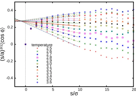
are linear fits for the initial linear segments of the plots. Temperature is given in the units of kBT/ε. . . 18 2.3 Bond vector correlation function of polymer chains with different stiffness.

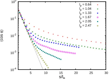
Points represent the simulation results for N=199 and T =3.1ε/kB. Horizon-tal axis is scaled by the corresponding persistence length lp, dotted line shows the exponential function e−s/lp_{. . . 21}

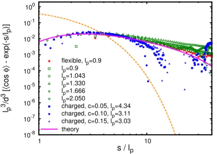
2.4 The residual non-exponential decay of the bond vector correlation function. The dashed and solid lines mark the exponential and non-exponential compo-nents of the bond vector correlation function (the first and the second terms in Eq (2.28)), respectively. The coefficients c_φ_·A =1.84_±0.04 and kl = 4.3_±0.07 were determined by fitting simulation data to theoretical predic-tion Eq (2.32). Persistence length lpis given in units ofσ, and concentration is units ofσ−3. . . 22 2.5 Flory characteristic ratio for polystyrene in cyclohexane at 34.5◦C (θ-solution)

(10)

2.6 Swelling ratio of simulated polymer chain consisting of 100 monomers. Lines show the best fit of simulation data by Eq (2.43) (solid line) and Eq (2.45) (dashed line). . . 29 2.7 Bond vector correlation function of simulated polymer chain with monomers

interacting via LJ potential (Eq (2.23), solid circles) and via special quasi-ideal potential (Eq (2.54), open circles). . . 34

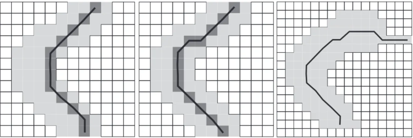
3.1 Molecule image after separation from substrate. Pixels belonging to the molecule are shown in gray. . . 43 3.2 (a). The shortest path between the molecule ends when edge weight

corre-sponds to its euclidean length. (b). The shortest path between the ends with the edge weight adjusted according to the distance from the border. (c). The result of ”tentacle” defects at molecule ends on the obtained central line. . . . 45 3.3 Individual molecules of polymer 1 were clearly resolved by tapping mode

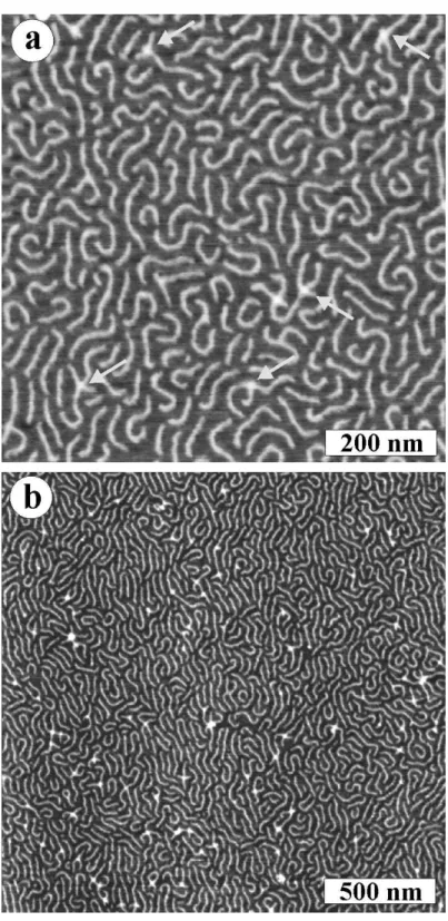
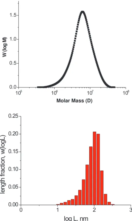
AFM. The higher resolution image (a) demonstrates details of the molecular conformation including crossing molecules indicated by arrows. The larger scale image (b) demonstrates the uniform coverage of the substrate. . . 50 3.4 (top) MALLS-GPC diagram presents molecular weight distribution of Sample

2. (bottom) The molecular length distribution (eq. 3.5) was measured by AFM for an ensemble of 3060 molecules. . . 51 3.5 Schematics of a brush-like macromolecule embedded in a melt of linear chains

with a degree of polymerization NB. Brush’s backbone and side chains have the degrees of polymerization NAand N, respectively. . . 55 3.6 Height AFM images of individual brush molecules embedded into monolayers

(11)

3.7 Dependence of the square root of the mean-square radius of gyration of pBA brush on the degree of polymerization of linear pBAs chains for different de-grees of polymerization of the backbone (NA). The solid lines are the best fit to the crossover equation 6 with a single set of two adjustable parameters A1=0.31±0.01 and A2=0.3±0.08. . . 58 3.8 Three conformational regimes of a brush-like macromolecule embedded in a

melt of linear chains with a degree of polymerization NB. The lower boundary of swollen test chain regime, NB=N2, is determined by the degree of poly-merization of the side chains (N), while the upper boundary of the ideal chain regime, NB=NA/N, also depends on the degree of polymerization of the brush’s backbone (NA). . . 58 3.9 The height image (a) of single molecules of four-arm pBA brushes was

ob-tained by tapping mode AFM using commercial HiRes probes (b). The probes were prepared by growing a forest of ultrasharp extratips wi th a radius down to 1 nm on top of a regular Si tip. . . 65 3.10 Schematic for a conformational transition of a multiarm brush molecule caused

(12)

3.11 The surface pressure-molecular area isotherm for the four-arm brush was mea-sured at T =23◦C. The mean molecular area(MMA)was determined for the number-average molecular weight Mn=5.5×106obtained by MALLS-GPC. The mean molecular area is the average area of a single brush molecule on the water surface. The points on the compression isotherm indicate compressions at which a monolayer was transferred onto mica forAFMstudies. Each point corresponds to an AFM image in Figure 3.12. . . 70 3.12 AFM observes the transition of the four-arm brush from a starlike to a disklike

conformation. The transition was caused by lateral compression of monolayer films on the surface of water. The height images correspond to different degrees of compression depicted in Figure 3.11. The cartoon in part d shows hexagonal ordering of disklike molecules stabilized by steric repulsion of adsorbed side chains. The cross-sectional profile in part e was measured along the dashed line in part c. . . . 71 3.13 Height images of the compressed linear brush (a) and four-arm brush (b). The

highlighted area in part b shows a domain with nearly perfect hexagonal order. The insets show 2D power spectral density measured for 1_×1µm2areas of the monolayers. Six peaks are clearly visible in the four-arm PSD, indicating the presence of hexagonal order in the system. . . 73 3.14 Angular dependence of the 2D power spectral density function P2(s)calculated

(13)

3.15 (A) Radial correlation function exemplified for the case of the four-arm brush molecule (1_×1µm2image). (B) The decays of the amplitude of the secondary maxima of C(R) as a function of distance for four-arm (circles) and linear brushes (squares) were fitted by an exponential function to obtain the transla-tional correlation lengthsξT =76 and 72 nm for the four-arm and linear brush, respectively. . . 75 3.16 The orientational correlation function decays exponentially to a finite number

on a short-range scale for the four-arm brush but decays to zero for the linear brush. For larger AFM images, both functions tend to zero at large distances. . 76 3.17 Conformational response of pBA brush-like macromolecules to adsorption on

(14)

3.18 Schematic of the spreading of a brush-like macromolecule on an attractive sub-strate. After adsorption, the macromolecule spreads to increase the number of monomeric contacts with the substrate. The brushlike architecture imposes constraints on the spreading process making it anisotropic and leading to ex-tension of the backbone. Along the brush axis, the wetting-induced tensile force f ∼=S_·d is supported almost entirely by the covalently linked backbone, where S is the spreading coefficient and d is the brush width. In the direction perpendicular to the backbone, the force is evenly distributed over many side chains, each bearing a f ∼=S_·δtensile force, whereδ is the distance between the neighbouring side chains. . . 80 3.19 Adsorption-induced degradation of macromolecules. a, The molecular

degra-dation of brush-like macromolecules with long side chains (n=140) on mica was monitored using AFM height imaging after each sample was exposed for different time periods (as indicated in the images) to a water/propanol (99.8/0.2wt/wt%) substrate. b, Schematics of an adsorbed macromolecule (left) which undergoes spontaneous scission of the covalent backbone (right). Side chains are shown in light grey, the backbone in dark grey. c, The cumulative length per unit mass, measured within an area of A=25µm2at a constant mass density of σ=0.08µgcm−2, was found to stay at an approximately constant value of Λ=9.6_±0.5µm f g₋1 throughout the scission process. d, The num-ber average contour lengths measured after different exposure times t (white circles) are fitted according to _L₋1_L

∞ =

1 L−L0 +

kt

(15)

3.20 Computer simulation of the scission process. a, The computer model assumes a constant scission probability P along most of the backbone; at the ends, P de-cays linearly to zero from x2=120nm to x1=40nm. This ensures the scission process stops at the experimentally observed L_∞= 40nm. b, Length distri-butions obtained by computer simulation for different time intervals t of the scission process (solid lines). The simulated distributions show good agree-ment with the distributions (data points) obtained by AFM on the same poly-mer/substrate system as used to obtain the images shown in Fig. 3.19a. The distributions are presented as the weight fraction of polymer chains of a certain number average contour lengthwith a resolution (bin size) of 50 nm. The ini-tial distribution function exactly corresponds to a realistic ensemble of 2,450 molecules acquired by AFM at t =0 with Ln=496nm and PDI = 1.52. . . 84 3.21 (a) On the surface of highly-oriented pyrolytic graphite, PBA brush-like

(16)

3.22 (a) A microscopic drop of a polymer-melt (volume_∼1nl, radius_∼100µm was scanned by AFM to measure the displacement L of the precursor-film edge and the distance r between the molecules within the film. The polymer melt is composed of (b) cylindrical brush molecules with (c) poly(n-butyl acrylate) side chains. (d) At later stages of spreading on mica one observed monolayer terraces at the foot of the drop with a thickness of 5 nm. . . 90 3.23 (a) AFM monitors sliding of the precursor monolayer of PBA brushes on the

(17)

3.24 (a) Animation of one of the spreading molecules demonstrates different modes of the molecular motion including translation of the center of mass, chain ro-tation, and fluctuations in the backbone curvature. The numbers indicate the observation time during the spreading process. (b) The trajectories of the center of mass of a group of 100 molecules (bold line) along with individual trajec-tories of three molecules (thin lines). The inset shows the path of one of the molecules in the frame of the precursor film by plotting the molecular trajec-tory relative to the center of mass of the group. (c) Mean-square intermolecular displacement_hr2_i=4D_inducedt was averaged for 100 molecules to determine the molecular diffusion coefficient Dinduced=1.3±0.1nm2/s. (d) Translational diffusion of 80 single brush molecules was monitored by AFM via interruptive scanning to determine two diffusion coefficients Dtherm =0.61±0.08nm2/s and Dtherm=0.10±0.03nm2/s at 10-minute () and 2-hour () intervals be-tween the consecutive scans, respectively. . . 94 3.25 The translational diffusion coefficient Dinduced in the precursor film increases

with the velocity of the film. This evidences the mechanically induced random-walk of molecules within the sliding film. . . 96 3.26 (a) Adsorption of brush-like macromolecules on surface results in

(18)

3.27 Schematic of the epitaxial adsorption of comblike molecules on graphite sub-strate: (a)HOPG substrates have a mosaic structure slightly disoriented mo-saic blocks with a spread of the _h0001_ic axis of 0.4_±0.1◦ in grade A and 0.8_±0.2◦in grade B; (b) Epitaxial adsorption of side chains leads to uniaxial alignment of polymer backbones along a particular crystallographic axis within the (0001)plane; (c) For example, if the side chains orient along the _h11¯20_i axis of the graphite lattice, this causes the backbone to orient along the_h11¯10_i axis. . . 102 3.28 AFM was used to obtain height images showing molecular organization of

spin-cast films of brush-like macromolecules on (a) graphite (grade A) and (b) mica substrates. The dashed circles and arrows in (a) highlight the ordered domains and their orientations; (c, d) angle distribution of molecules relative to the horizontal axis of the AFM images was measured on graphite and mica, respectively. . . 104 3.29 Precursor films prepared from spontaneous spreading of the comblike molecules

on (a) graphite (grade A) and (b) mica. (c) On graphite, molecules show a nar-row angle distribution measured relative to the horizontal axis. In contrast, molecules on mica reveal a broad (isotropic) angle distribution. (d) While the two-dimensional orientational order parameter S=2_hcos2θ_{i −}1 levels of on graphite at S=0.75; it rapidly drops to zero on mica. . . 105 3.30 Two large-scale AFM height images demonstrate examples of different

(19)

3.31 (a-d) Higher magnification height images were measured in different areas of the precursor film on graphite. The images reveal a lack of correlation between the flow direction and orientation of the flowing molecules. This behavior is clearly seen in (d) showing differently oriented domains in the same area of the precursor film. (e) From the cross-sectional profile along the dashed line in (d), one determines a terrace thickness of 0.32_±0.05 nm which matches with the AB interlayer spacing c=0.335 nm of HOPG (see Figure 3.27a). . . 109 3.32 AFM was used for real-time imaging of the shift in molecular orientation upon

crossing a grain boundary during spreading of pBA brushes on graphite (grade A). The micrographs (a) and (b) represent phase and height AFM images that are taken from the same sample area in order to visualize the grain bound-ary between two mosaic blocks (Figure 3.27a). The grain boundbound-ary shows no height contrast and becomes visible only in the phase image (white arrow). Then white dashed lines were used to highlight the grain boundary in the sub-sequent height images from (b) to (f). The dotted lines in images (b-f) indicate the average molecular orientation within the two domains. The angle between the directors was measured to be about 120◦. . . 110 3.33 Diffusion coefficients were measured on two HOPG substrates (grade A and

(20)

(21)

List of Tables

(22)

(23)

Chapter 1 Introduction

(24)

dif-ferent polymers. Despite the fundamental and practical significance of theθ-point, behavior of a polymer in aθ-solution is still poorly understood.

Following the analogy with theory of gases one may assume that because of compensation of attractive and repulsive parts of monomer interactions, a polymer in a θ-solution behaves as if there were no interactions at all, that is, as an ideal polymer. Even though this is not correct, conformations of a polymer in a θ-soluton are often described as quasi-ideal, that is the state where the conformation of a real polymer can be treated as ideal for all practical purposes. In Chapter 2, we show that this classical approach results in inaccurate predictions of polymer size and structure, because it neglects the effect of polymer connectivity on monomer interactions. Polymer connectivity induces the long range correlations along the chain, which are completely absent from the ideal chain as well as from the classical descriptions of polymer in the θ-state. Thus, we demonstrate that the ideal chain can not be used to model polymers inθ-solvents. We have found that the mean square size of the chain in aθ-solvent has a large correction_∼√N to the linear term.

If monomers were not connected, the compensation of their interactions would lead to an ideal solution of monomers. But, monomers are connected and we have proven that their connectivity causes the qualitatively different behavior of polymers inθ-solutions.

(25)

indi-vidual molecules, which is hardly possible in the bulk. It is therefore reasonable to address the analysis of visualized macromolecules on a surface obtained by means of scanning probe microscopy.

An outstanding method for studies on the nanometer scale is the Atomic Force Microscopy (AFM). It can be used for visualization of surface morphology, probing physical properties, and maskless nanolithography. Visualization by AFM is the most significant area of applica-tions due to its high spatial resolution, which for soft polymers ranges over 1-10 nm. In this range of length scales, materials are full of intriguing electronic, magnetic, and optical proper-ties promising new advances in lithography, data storage, photonics, and molecular electronics. Furthermore, the imaging conditions do not require any sample modification or special envi-ronment such as those needed for electron microscopy. As such, native structures can be visu-alized in their natural medium, which is especially vital in biology. Not only is AFM effective at small length scales, it is also able to visualize larger structures such as crystallites, micelles, and blends making it possible to establish direct correlations between the molecular structure and macroscopic properties. Along with visualization of static structures, AFM is able to mon-itor various processes such as crystallization and conformational transitions enabling studies of dynamic properties of polymeric materials.

(26)

molecules, accounting for the image discreteness and low resolution, and multiple image anal-ysis for polymer dynamics studies.

We have used molecular brushes as a convenient model polymers that have well controlled length and stiffness to produce clear images upon visualization. The new method of image analysis has then been applied to molecular brushes.

The developed software was first applied to characterize molecular dimensions. Thus we have measured the length of macromolecules and their number density on the surface, and by knowing the mass concentration we have been able to accurately estimate the molecular weight.

The ability to measure molecular dimensions was applied to analyze the extension of the classical Flory theory of mixing to planar melts. Using our method we have studied the binary mixtures of molecular brushes and linear polymers. We have found that swelling of molecular brushes in the melt of linear chains can be described by an equivalent linear chain made of NA/N monomers, where NA is the backbone degree of polymerization, and N is the side chain degree of polymerization. A generalized Flory theory of mixing has been suggested, based on the analysis of our observations.

The next step in our studies of polymers on the surface was the analysis of more complex systems of multiarm molecular brushes. For these systems we have calculated the polydisper-sity and studied the ordering on the surface. We have found that multiarm molecular brushes undergo the sharp conformational transition from an extended to compact state. This transition narrows the molecular size distribution and induces orientational order.

(27)

and on the strength of adsorption, characterized by the surface tension.

It is also very interesting to observe the dynamic behavior of molecular brushes. We have watched the molecular motion in the precursor layer of the droplet spreading on graphite, and measured the coefficients of polymer diffusion relative to the surface and to the precursor film. Comparing these coefficients we have discovered that the main mechanism of mass transport in the precursor layer is the molecular motion induced by the plug flow of the polymer, and that the contribution of thermally driven diffusion is minor.

(28)

(29)

Chapter 2 Long range correlations in a polymer

chain due to its connectivity

2.1 Introduction

Polymer chains can have different conformations depending of the interaction between their monomers. If interactions are predominately repulsive, as in the case of good solvent solutions, polymers swell, while if their interactions are attractive, as in the case of poor solvent, chains are collapsed. Between these two cases there is a special condition, calledθ-point, in which the average pairwise interaction between monomers is zero and the chain is almost ideal. Similar compensation of attractive and repulsive parts of monomeric interactions occurs in polymer melts and concentrated solutions. In semidilute solutions the pairwise interactions vanish on length scales larger then the correlation length ξdue to the screening of excluded volume by surrounding chains. Polymers without pairwise interactions, as in θ-solvent and melts, are traditionally described by the ideal chain model [3–14].

(30)

local steric hindrance) lead to exponentially decaying correlations in directions of vectors ai and aj of bonds i and j separated by the distance s=a|i− j|along the chain

h(s) = 1

a2

aiaj

∼e−s/lp _(2.1)

where lpis the persistence length and a is the bond length. Rapid decay of bond vector correla-tions leads to the random walk statistics of the chain on length scales larger than the persistence segment length lp. The concept of the persistence length is widely used for characterization of the polymer flexibility [15–19]. Single stranded DNA (lp≈2nm) is an example of a flexible chain, and double strained DNA (lp≈50nm) is a common example of a semiflexible polymer. The assumption of ideality of chains in melts and concentrated solutions was recently demonstrated to be incorrect [20]. Using both computer simulations and theoretical estimates it was shown that bond vector correlation function (Eq (2.1)) in melts and semidilute solutions decays as a power law

h(s)_∼s−3/2, (2.2)

This unexpectedly slow decay of correlations was explained by the effect of correlation hole [21], which leads to relative compression of the chain with respect to its ideal state.

(31)

other leading to zero effective second virial coefficient. The main result of this chapter is that connectivity of chain monomers leads to additional correlations in their relative position in space causing additional interaction between these monomers as compared to the case of unconnected monomers. In the latter case the effect of hard core is canceled by attractive well at the compensation point. The connectivity of monomers in the chain results in a slight shift of the probability of the two monomers to be within the range of the attractive well of the interaction potential. The magnitude of this shift depends on the distance between the two monomers along the chain contour. This probability shift leads to a nonzero effective interaction of two monomers belonging to the same chain.

Another manifestation of the new effect is the large correction term _∼√N to the expected in θ-solvent linear dependence of the mean square polymer chain size R2 on its degree of polymerization N. This change of polymer size can be observed experimentally by measuring the rate of approach of the Flory characteristic ratio Cnto its limiting value C∞with increasing molecular weight M.

(32)

monomers in contact. This effect leads to corrections of chain size and induces long range correlations of chain segment orientations.

It is well known that conformations of a polymer chain at a θ-point are not ideal [13, 14, 22, 23]. The earlier studies discussed the renormalization of pairwise monomeric interactions caused by three (and higher) body contacts. It can be shown [14] that this short-range renor-malization leads to the shift of the effectiveθ-temperature relative to the Flory’sθ-temperature of the ”gas of monomers”. The corrections to the polymer size at the new shiftedθ-temperature renormalize the effective Kuhn length. The next order non-linear corrections [14] are on the order of_∼y/(1+y log N), where y is proportional to the third virial coefficient [14]. The bond vector correlation function due to this correction _∼ log2N

N2₍₁₊_{y log N}₎2 decays faster and is therefore

less important than our new prediction_∼N−3/2due to connectivity-induced correlations. The logarithmic correction to the chain size decays slower than our connectivity-induced correction

∼N−1/2and therefore may dominate for very long chains.

(33)

long range correlations in polymers.

2.2 Bond vector correlation function

2.2.1 Telechelic model

In the ideal chain model there are no long range correlations in orientation of polymer seg-ments. Such correlations appear as a result of interactions between chain monomers. In or-der to study the effect of interactions on the chain segment orientations we first consior-der the telechelic chain model consisting of a Gaussian chain of N Kuhn monomers, with only two end monomers interacting with each other via a short-range potential U(r), depending only on the distance between these monomers (the end-to-end vector r of the chain)

r=

∑

N_i₌₁ai. (2.3)

Here aiare bond vectors with average length a equal to its Kuhn length a=b. This model will be generalized in section 2.2.2 in order to take into account interaction of all monomers of the real chain.

In the simplified telechelic chain model the correlation function hL(s) of the two bond vectors i and j

hL(s) = 1 a2

a(si)a(sj)

(2.4)

does not depend on their positions si and sj along the chain contour (hL(s) =hL), nor on the distance along the chain s=a_|i₋j_|between them, since the probability of chain conformation depends only on the sum of all bond vectors a(si), that is on the end-to-end vector, Eq (2.3). We calculate the correlation function hL in two steps:

(34)

end-to-end vector r (see Appendix 2.A for details)

HL(r) = 1

a2 ha(si)a(sj)i

r=

r2₋bL

L2 . (2.5)

where L is the chain contour length and b is the Kuhn length. According to this expression the two bond vectors are not correlated only when r is equal to the root-mean-square end-to-end distance of this chain, bL. They have opposite preferential orientation (with HL(r)<0) if the chain is compressed, r2<bL, and the same orientation (along the end-to-end vector r, with HL(r)>0) for stretched chain, r2>bL.

U(r)

r

i

j

Figure 2.1: Telechelic chain model

Second, we average the result, HL(r) (see Eq (2.5)), over different end-to-end distances r with the monomer contact probability distribu-tion to obtain hL Eq (2.4) (see Appendix 2.B)

hL= 1

a2haiaji=

3 2π

3/2

B b1/2L5/2+

5 2

A

b3/2L7/2+···

,

(2.6)

where B is the second virial coefficient

B=₋

Z

f(r)d3r, (2.7)

the coefficient A is

A=

Z

f(r)r2d3r. (2.8)

and f(r)is the Mayer f -function:

(35)

Note that, as expected, the bond vector correlation function does not depend on location of the bond vectors along this telechelic chain nor on their separation s along the chain (number of bonds between them), but only depends on the contour length L between two interacting monomers of the chain.

In classical models of polymers [10] the bond vector correlation function hL includes only the second virial coefficient B term:

hL =

3 2π

3/2

B

b1/2L5/2, (2.10)

Therefore, classical theories predict the absence of the long range correlations of polymer segments orientations inθ-solution.

The most important conclusion from this simple model of telechelic chain is that at the

θ-point (with zero second virial coefficient B=0) the correlation between bond vectors decays as a power of the curvilinear distance L along the polymer contour between two interacting monomers_ha(si)a(sj)i ∼AL−7/2in the telechelic chain.

2.2.2 Polymer with all interacting monomers

A more realistic description of a polymer is a chain, with all N+1 monomers interacting with each other. The bond vector correlation function h(i,j) = _a12ha(si)a(sj)i of two bonds,

separated by the distance s=a_|i₋j_|along the chain can be found by taking the sum of con-tributions of all loops formed by pairs n and m of interacting monomers with sn<si<sj<sm which contain bond vectors a(si)and a(sj):

h(i,j) =

∑

n<im>

∑

j,i<j

(36)

Substituting the function HL from Eq (2.6) and replacing the summation in Eq (2.11) by the integration, we obtain

h(i,j)_≃

3 2π

3/2

Bg_1/2(i,j) + 5

2Ag3/2(i,j) +···

, (2.12)

where

gk(i,j)≡ Z si

0 dsn

Z L sj

1 bk₍_s

m−sn)k+2 dsm=

1 k(k+1)bk

"

1

(sj−si)k− 1 sk_j −

1

(L₋si)k

+ 1

Lk

#

.

(2.13)

We see, that the bond vector correlations decay as a power law of the distance s=_|sj−si|= a_|j₋i_|along the chain between bonds i and j. For internal bonds (that is, when 1_≪i< j_≪N) of a sufficiently long chain (N_≫1) atθ-condition (B=0), we find power law decay of the correlation function with the exponent k=3/2

h(i,j) = 1

a2haiaji=h(s)∼s

−3/2

(θ-solvent) (2.14a)

(as long as A₆=0). If one of these bonds is at the chain end (si−ε=0) we have

h(0,j) = 1

a2ha(0)a(sj)i ∼(sj−ε)− 3/2

−s−_j3/2_∼s−_j5/2 (end monomer,θ-solvent). (2.14b) If both bonds are at the opposite chain ends we recover the result of the previous subsection h(0,L) = _a12ha(0)a(L)i ∼L−7/2. In good solvent (B>0) the bond vector correlation function

decays with exponent k=1/2

(37)

Notice, that expansion coefficients B and A in Eq (2.12) depend on the shape of interaction potential. Although it is possible to design the special potential U(r) in order to have B=

A=0, the higher order term would still be non-zero leading to power law decay with a higher exponent.

2.2.3 Connectivity induced modification of monomeric interactions

An alternative way of deriving the bond vector correlation function h(s) for a polymer in a good solvent is from the mean square distance between monomers i and j

hr2_i=a2

* _j

∑

k,l=i

akal

+

=

j

∑

k,l=i

h(b_|i₋j_|)_≃2 Z ja

ia ds1

Z s₁ 0

h(s1−s2)ds2, (2.15)

Summation over bond vectors k and l was replaced by integration over chain contour coor-dinates s1 and s2 in the last part of Eq (2.15). Taking two derivatives of the mean square end-to-end vector (Eq (2.15)) with respect to contour length between monomers s=a_|i₋j_|, we find

h(s)_≃2d 2_h_r2_i

ds2 . (2.16)

The size of a polymer in the vicinity of theθ-point is given by the expression [10, 24, 25]

hr2_i=bs 1+4

3 s1/2 b1/2

B b3+. . .

!

(2.17)

where b is the Kuhn monomer size. For simplicity assume it equal to bond length for flexible chains (b=a). We will consider semiflexible chains with b>a in section 2.2.5. Substituting expression (2.17) into Eq. (2.16) we get the bond vector correlation function

h(s)_≃ B

b5/2 1

(38)

in agreement with the results of the previous subsection (Eq (2.14c)). Thus, no long range correlations are expected at theθ-point (B=0), according to the classical approach.

In order to study correlations at the θ-conditions one should take into account that in ad-dition to the direct monomeric interactions, described by the potential U(r), there are indirect elastic interactions that propagate along the chain. The total effective interaction potential of two monomers separated by the distance r is Utot(r) =U(r) +Us(r), where Us(r) is the spring-like potential due to the chain section between these monomers

Us(r) = 3kBT

2sb r

2_. _(2.19)

Mayer f -function reflects the difference between statistical weights (Boltzmann factors) of states with interactions and without them (U(r) =0). Since the Us(r) is the only effective potential between monomers at large distances r, when U(r) =0, the effective Mayer function of these monomers connected into a chain is

fs(r) =e−Utot(r)/kBT−e−Us(r)/kBT (2.20)

Substituting this equation into Eq (2.7) we find the effective virial coefficient B(s), which depends on the separation s of the interacting monomers along the chain contour. At large s_≫b one can expand this function in powers of 1/s

B(s) =₋

Z

fs(r)d3r≃ − Z

1₋3r 2 2sb+···

e−U(r)/kBT₋₁

d3r= =₋

Z

e−U(r)/kBT₋₁_d3_r₊ 3

2sb Z

r2e−U(r)/kBT₋₁_d3_r₌ _(2.21)

=₋

Z

f(r)d3r+ 3

2sb Z

r2f(r)d3r=B+ 3A

2sb+···

(39)

derived assuming that chain is flexible (lp.a). A more general case of semiflexible chains with persistence length lp&a will be discussed in Section 2.2.5. Although B=0 in theθ-solvent, the effective second virial coefficient B(s) does not vanish at the θ-condition. Substituting this expression into Eq (2.10), and summing contributions from all pairs of monomers (see Eq (2.11)) we get∗

h(s)_≃ B

b5/2 1 s1/2+

3 2

A b7/2

1

s3/2. (2.22)

which is equivalent to Eq (2.12) for 0_≪si<sj≪L.

Note, that here we consider only the two-body interactions, as the effect under study is stronger than the contribution of multibody interactions. Also, note that since B(s)depends on the separation s between monomers, it vanishes at different temperatures for different s. In general it is impossible to suppress the long range correlations (that is to have both B=0 and A=0), except in certain special cases as described in Appendix 2.C.

2.2.4 Computer simulations

To test our analytical predictions by computer simulations we employ the coarse-grained con-tinuum bead-spring model of polymer chains. A polymer in this model consists of N+1 soft-sphere monomers, interacting with each other via the truncated and shifted Lennard-Jones (LJ) potential

ULJ(r) =

       4ε σ r 12

−σ_r6

−4ε

" σ rc 12 − σ rc 6#

r<rc

0 r>rc

(2.23)

∗_{Note, that the effective B}₍_s₎_{can not be substituted for B in Eq (2.17). In order to obtain the correct polymer}

(40)

where r is the distance between monomers and rc is the cutoff radius (we use rc=2.5σfor all simulations). Chain connectivity is modeled by the finitely extensible nonlinear elastic (FENE) interaction potential between adjacent monomers (in addition to the LJ potential)

UFENE(r) =− 1

2kFENER 2 0ln

1₋ r 2

σ2_R2 0

(2.24)

where kFENE is the spring constant and R0 is the maximum extension of the bond, at which the interaction energy becomes infinite. In this work we choose R0=2σand kFENE=10ε/σ2, which minimizes the N-dependence of theθ-temperature [26]. New conformations are gener-ated using the standard method of constant temperature (NVT ensemble) molecular dynamics. Initial configurations were created as random self-avoiding walks, and then equilibrated for at least 10τR, where τR is the longest relaxation time, determined from the decay of the chain end-to-end distance autocorrelation function.

-0.4 -0.2 0 0.2 0.4

0 5 10 15 20

(s/a) 3/2 〈 cos φ〉 s/σ temperature 2.5 2.6 2.7 2.8 2.9 3.0 3.1 3.2 3.3 3.4 3.5 3.6

(41)

In fig. 2.2 we present the bond vector correlation function

hcosφ_i= 1

a2ha(si)a(si+n)i= 1 N₋n

N−n

∑

i=1

h(i,i+n) (2.25)

averaged over all pairs of monomers separated by segments of length s and multiplied by the number of monomers, s/a, between the two bonds to the power 3/2. The average in Eq (2.25) is dominated by the internal chain sections with h(i,j)_≈ B_|sj−si|−1/2b−5/2+

5

2A|sj−si|−

3/2_b−7/2_{, therefore we expect that} ₍_s_/_a₎3/2_h_cos_φ_{i ∼} 5

2A+Bsb should have lin-ear dependence on the curvilinlin-ear distance s between two bonds. The temperature dependence of A(T)can be represented∗as A(T) =A(θ)₋s0bB(T)with a numerical constant|s0/a| ∼1. This gives

s

a

3/2

hcosφ_{i ∼}A(θ) +B(T) (s₋s0)b (2.26) Fitting the linear sections of the(s/a)3/2_hcosφ_icurves we notice that lines for different tem-peratures cross at one point with s0/a_{≃ −}0.86, as expected from our analysis.

2.2.5 Semiflexible chains

In this section we will discuss the long-range correlation effect in semiflexible chains with per-sistence length lplarger than bond length a.lp≪L. So far we considered flexible polymers with lp.a and Gaussian probability of contact between all pairs of monomers. However, the probability of monomeric contacts for semiflexible chains with lp&1 is strongly reduced at monomeric separations shorter than _∼5lp[27–29]. The reduction of contact probability sup-presses the effect of the long-range correlations, and short chain segments behave as elastic rods with exponential decay of correlations (Eq (2.1)). To account for this fact we need to in-clude the small s contact probability in the effective Mayer f -function of connected monomers

(42)

Eq (2.20):

fp(r,s) =ζ(s,r)f(r,s), (2.27) whereζ(s,r)describes the deviation of contact probability between i and j monomers from the Gaussian approximation. The asymptotic limits ofζ(s,r=0)are evidently lim

s→0ζ(s) =0 and lim

s→∞ζ(s) =1. For small r/s→0 we can expand the new monomer contact probability function

and expect that h(s)_≈ζ(s)h0(s), where h0(s)denotes the bond vector correlation function of flexible chains, as given by Eq (2.22).

The complete bond-vector correlation function for semiflexible chains can be represented as the sum of short-range and long-range contributions:

hcosφ(s)_i=e−s/lp₊_c

φζ(s)h0(s) (2.28)

where c_φ is the normalization coefficient.

The approximate form of the ”stiffness function” ζ(s)can be obtained by considering the formation of a loop in a semiflexible chain of length s. The bending energy in this case is [30]

E(s) =kBT lp

2 s Z

0

κ(s′)2ds′. (2.29)

whereκ(s)is the curvature (inverse of the radius of the circle that describes the bend).

In order to test our idea about the nature of the crossover (Eq (2.28)) from exponential to power law decay of the bond vector correlation function, we define ζ(s)as the Boltzmann weight of the loop of length s:

ζ(s) =exp

−E(s)

kBT

=exp

−kllp

s

(2.30)

where kl is the numerical constant to be found from our simulation results∗.

(43)

The chain stiffness in our simulations is introduced through the bending potential

U(φ) =u_φ(1₋cosφ) (2.31)

whereφ is the angle between the neighboring bonds i and i+1, and u_φ is the stiffness of the bending potential. The persistence length of such chains depends on u_φand for large u_φ_≫kBT becomes proportional to it: lim

u_φ→∞lp=σuφ/kBT .

10-4

10-3

10-2

10-1

100

5 10 15 20 25 30

〈

cos

φ〉

s/l_p

l_p = 0.64

lp = 1.04

l_p = 1.33

l_p = 1.67

lp = 2.05

l_p = 2.47

Figure 2.3: Bond vector correlation function of polymer chains with different stiffness. Points represent the simulation results for N=199 and T =3.1ε/kB. Horizontal axis is scaled by the corresponding persistence length lp, dotted line shows the exponential function e−s/lp.

The magnitude of the long-range correlation effect decays with increasing stiffness. This can be explained by the decrease of the probability to form a loop between the interacting monomers. The growing value of the persistence length lp leads to an overall decrease of polymer concentration c∗ inside the volume _hr2_i3/2 _∼(slp)3/2 occupied by the segment of length s, and the probability of pair contacts decays correspondingly c∗_∼ d3

hR2_i3/2 ∼

d3

(slp)3/2.

(44)

The magnitude of the long-range correlations effect is proportional to the probability of contact between the two monomers (estimated as the ratio of the monomer interaction volume d3 to the pervaded volume of the segment(slp)3/2).

10-8 10-7 10-6 10-5 10-4 10-3 10-2 10-1 100

1 10

lp 3 /d 3 [

〈 cos φ〉 - exp(-s/l p )]

s / lp flexible, l_p=0.9

l_p=0.9 l_p=1.043 l_p=1.330 l_p=1.666 l_p=2.050

charged, c=0.05, l_p=4.34 charged, c=0.10, l_p=3.11 charged, c=0.15, l_p=3.03 theory

Figure 2.4: The residual non-exponential decay of the bond vector correlation function. The dashed and solid lines mark the exponential and non-exponential components of the bond vec-tor correlation function (the first and the second terms in Eq (2.28)), respectively. The coeffi-cients c_φ_·A=1.84_±0.04 and kl =4.3±0.07 were determined by fitting simulation data to theoretical prediction Eq (2.32). Persistence length lpis given in units ofσ, and concentration is units ofσ−3.

Fig. 2.3 shows the decay of the bond vector correlation function for semiflexible chains with different lp. The coefficient of the Lennard-Jones potential (Eq (2.23)) was set to ε=

(45)

monomer contact probability on the persistence length d3/(slp)3/2= (d/lp)3(lp/s)3/2. Thus for a given value of s/lpthe factor(lp/d)3_{is expected to collapse the data. For the short-ranged} LJ potential the interaction radius is about the size of the monomer d/σ_∼1. The extracted exponential decay component of the_hcosφ_i(s)is shown in (Fig. 2.4) by the dashed line e−s/lp_,

and the theoretical expectation for the long-range decay Eq (2.28)

h(s)₋exp(s/lp) =cφζ(s)h0(s) =cφe−

kllp s

3 2π

3/2

·5₂ A

b7/2s3/2 (2.32)

is shown by the solid line. The coefficients obtained by fitting the numerical data are c_φ_·A=

1.84_±0.04 and kl =4.3±0.07. The data for the flexible chain are shown on the same plot for the guidance purposes, to illustrate the universal nature of the long-range correlations in polymers. Since the regular definition of the persistence length (see Eq (2.1)) is inapplicable for flexible chains, the numerical data were scaled using the empirical value of lp =0.9σ required to collapse them with the results for the semiflexible chains.

The long range intramolecular correlations in a dilute solution of charged polymers are the natural consequence of the long range electrostatic interactions. In semidilute polyelec-trolyte solutions these interactions are screened by charges of neighboring chains and by coun-terions. To compare the behavior of charged polymers with our previous findings we dis-cuss the coarse-grained model, in which the semidilute polyelectrolyte solution is consid-ered as the melt of chains, consisting of correlation volumes (blobs). Each such blob of size

(46)

The results of the molecular dynamics simulation∗for the bond vector correlation function of polyelectrolytes chains in semidilute solutions are shown in Fig. 2.4 with solid symbols. This function also exhibits long-range correlation. The corresponding curves can be collapsed with our results for neutral semiflexible chains by associating the range d of interactions with correlation lengthξ leading to the scaling factor l3_p/d3_≈l3_p/ξ3. For the solutions of concen-trations c=0.05σ−3, 0.10σ−3and 0.15σ−3we have found the values of the cube of the ratio of persistence length to correlation length l3_p/ξ3 to be 1.1_±0.1, 1.2_±0.1 and 1.3_±0.1, cor-respondingly. The ratio l3_p/ξ3 increases with concentration, which is in agreement with the predictions made in ref. [16].

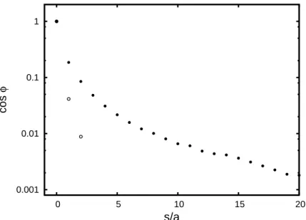
Significant deviation from the exponential decay of the bond vector correlation function begins at monomer separations of s_≈4_÷5lp, as can be seen in the Fig. 2.4. The magnitude of the correlations falls as _∼0.01l3_p at this crossover point. This decreasing magnitude of the effect makes observations of the non-exponential decay of the bond vector correlation function in polymers with large persistence length, such as polyelectrolytes increasingly more difficult.

2.2.6 Bond correlation function: Summary

In order to emphasize the two ingredients necessary for the power law decay of the bond-vector correlations let us examine another approach that includes monomer connectivity, such as the perturbation theory [11, 25], based on the Edwards model of polymer chain [4]. Al-though Edwards model includes monomer connectivity, the interactions between monomers are approximated by theδ-function†potential [4, 7, 10]

f(r) =₋Bδ(r). (2.33)

∗_{Details of this simulation are given in Ref. [33]} †_Here_δ₍_r₎_{is the 3-d Dirac}_δ-function,_δ₍_r_{) =} δ(r)

(47)

Due to the zero-range of the δ–function potential, the effect of connectivity on the monomer interactions vanishes (A=R

r2f(r)d3r=0) and B(s) =B (Eq (2.21)).

In order to account for the long-range renormalization of the monomeric interactions and thus correctly describe the macromolecular conformation, a polymer model has to meet two conditions. (i) The model must consider the fact that monomeric units are connected. (ii) The model must take into account the finite (non-zero) range d>0 of the monomeric interactions. Note that the Flory class of polymer models violates the first condition (ignores the monomer connectivity), while the Edwards class of models violates the second condition (finite range of interactions) and therefore both predict no long-range bond-vector correlations at theθ-point.

2.3 Polymer size

Polymer chain at theθ-condition is usually used as the reference state in the analysis of poly-mer conformations [34–41]. The dependence of the mean square end-to-end distance of the polymer at theθ-temperature on the number n of bonds in it is described by the characteristic Flory ratio

Cn= R2

l₀2n (2.34)

where l₀2n is the end-to-end distance of the corresponding freely-jointed chain [42]. The ideal chain model predicts that the characteristic ratio quickly approaches its asymptotic value C_∞ with increasing n as C_∞₋Cn ∼n−1 [2, 43]. Long range correlations in the polymer chain described in the present chapter lead to much weaker dependence, C_∞₋Cn_∼n−1/2_∼N−1/2, where N is number of Kuhn segments of length b.

The polymer size in aθ-solution can be found from Eqs (2.15) and (2.22):

R2_θ(N) =b2N₋3 2b

(48)

1 2 3 4 5 6 7 8 9

10 102 103 104 105

Cn

M/M₀ 0.1 1.0 10.0

10 102 103 104 105 C∞

− C

n

M/M₀

Figure 2.5: Flory characteristic ratio for polystyrene in cyclohexane at 34.5◦C (θ-solution) [44]. For polystyrene the monomer length l0≈1.54 ˚A and its mass per bond is M0=52g/mol. where L=Nb. Similar _∼√N deviation from the ideal scaling R2_g(N)_∼N is derived in Ap-pendix 2.D from the bond vector correlation function.

The characteristic Flory ratio, Cn, of a linear chain can be expressed in terms of a mean square radius of gyration of a polymer at theθ-point:

Cn= 6R

2 g l₀2(M/M0)

(2.36)

where M0is the molar mass per bond. From Eq (2.35) we obtain the expression for the charac-teristic ratio which is a linear function of N−1/2_∼M−1/2, where C_∞is defined as C_∞=lim

n→∞Cn

C_∞₋Cn∼ 3 2

A

b5√_N (2.37)

(49)

molecules. To analyze the rate of this saturation we plot the difference of Cnfrom the limiting value C_∞. The log-log plot of this difference is presented in the inset in Fig. 2.5. The least-square fit of the data to the power law gives C_∞₋Cn = (32.0±2.2)(M/M0)−0.54±0.03. The measured exponent is in excellent agreement with the value of₋1/2 predicted by our theory confirming the validity of Eq (2.35). Similar N−1/2 dependence has been also obtained in Ref. [22] for the inner chain segments using the self-consistent mean-field approach.

2.4 Swelling ratio

Excluded volume interactions between monomers lead to either swelling or collapse of poly-mer chains relative to their ideal states [10,24]. For the classical models of a polypoly-mer chain with N Kuhn segments of length b the equation for the mean square swelling ratio α2=6R2_g/Nb2 can be written as

α2₌_c 0+

c1z

α3 + C

α6 (2.38)

where interaction parameter z is defined [10] as z=₂_π3_b2 3/2

N1/2B.

Dimensionless coefficients c0 and c1are model-specific and C is proportional to the third virial coefficient (renormalized by the 4-th and higher order virial coefficients).

Swelling factor in Eq (2.38) is defined relative to the size of the ideal chain. Since this size is not known neither experimentally nor numerically, we define the swelling ratioβrelative to theθ-state, that is the state with z=0:

β=Rg/Rθg=α/αθ, (2.39)

whereα_θis defined by equation (2.38) with B=0:

(50)

The interaction parameter z depends on the intramolecular second virial coefficient B. We will use the known temperature dependence [8] of this coefficient to analyze the computer simulation results and redefine the interaction parameter as

z=c2τN1/2b3 (2.41)

where c2is the numerical coefficient and the reduced temperatureτis defined as

τ=

  

 

(T₋T_θ)/T_θ at T <T_θ

(T₋T_θ)/T at T >T_θ

(2.42)

Here we use different expressions for τ depending upon whether the temperature is above or below the θ-temperature T_θ_≈3.1. The reason for this choice is that τ may be thought of as a normalized interaction parameter which varies from ₋1 in poor solvent conditions (T _→0), through 0 at T =T_θ where the chain is neither swollen nor collapsed (β=1), to 1 in good solvent conditions (T _→∞). Eq (2.42) guaranties that the limiting behavior of τis achieved while not changing the form ofτat temperatures close to T_θ.

To obtain the explicit form of z(β)we subtract Eq (2.38) from (2.40) to exclude c0and then substituteα=α_θβfrom Eq (2.39):

z=A1β5−(A1−A3)β3−A3β−3 (2.43)

This equation depends on two dimensionless coefficients, A1 =α5_θ/c1 and A3=C/ c1α3_θ

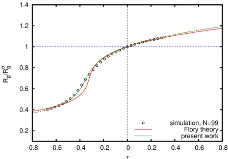
. The best fit of the simulated swelling data is shown in fig. 2.6 is shown by the open circles with A1=9.02 and A3=0.46.

(51)

0.2 0.4 0.6 0.8 1 1.2 1.4

-0.8 -0.6 -0.4 -0.2 0 0.2 0.4 0.6 0.8

Rg /R g θ τ simulation, N=99 Flory theory present work

Figure 2.6: Swelling ratio of simulated polymer chain consisting of 100 monomers. Lines show the best fit of simulation data by Eq (2.43) (solid line) and Eq (2.45) (dashed line).

account for the effect of monomer connectivity on the monomeric interactions, being based on assumptions either of mean-field model of cloud of unconnected monomers or of the Edwards model of infinitely thin chain with d/b_→0. The ratio d/b is not negligibly small for real chains. The thickness for most flexible hydrocarbon polymers is comparable to the Kuhn segment length, d/b_∼0.2_÷0.3. Connectivity of monomers with finite interaction range d into a chain leads to a new term A′/α4 in addition to three terms in Eq (2.43) (as shown in Appendix 2.E)

α2₌_c 0+

c1z

α3 + A′

α4+ C

α6. (2.44)

The corresponding expression for fitting the simulation data can be obtained similarly to Eq (2.43)

z=A1β5−(A1−A2−A3)β3+A2β−1−A3β−3 (2.45)

where A2= A

′

c1αθ. The best fit of numerical data to this equation is shown in Fig. 2.6 (dashed

(52)

curves in fig.2.6, the additional term (A′/α4) in Eq (2.44) is important in moderately poor solvents, and gives only weak corrections in the asymptotic regimes at_|z_{| ≫}1.

2.5 Conclusions

We have analyzed the conformations of linear macromolecules inθ-solution and shown that they are non-universal. Chain size and correlation of chain segments on all scales up to the size of the whole chain depend on the details of the intermonomeric potential. We have shown that polymer atθ-point does not have ideal-like conformation and is characterized by the long-range correlations. Correlation of chain segment orientations _haiajidecay as power law, except for semiflexible polymers, in which case power law decay can be masked by the initial exponential decay on length scales smaller than the length of several persistence segments. The deviations of the dependence of mean square chain size on the polymerization degree from the ideal law R2(N)₋b2N_∼√N are much larger than N−1 correction predicted by the classical theories. We explain this non-universal behavior by the effect of monomer connectivity and non-zero range of interactions. Classical description of the θ-state of a polymer chain can be recovered in the limit of point-type monomeric interactions (characterized by the delta-function form of the Mayer f -function f(r) =kBT Bδ(r)).

(53)

B(s)_∼s−1. This two-body interaction alone can introduce the long range correlations with a s−3/2dependence, similar to the connectivity effect (see Eq (2.22)), but with an opposite sign. The two effects may partially cancel or screen each other, depending on the magnitude of the coefficients B and A, determined by the chemical structure of monomers.

2.6 Acknowledgments

We would like to acknowledge financial support of National Science Foundation under grants CHE-0616925 and CTS-0609087, National Institutes of Health under grant 1-R01-HL0775486A and NASA under agreement NCC-1-02037.

2.A

Bond vector correlations for fixed end-to-end vector

Consider a flexible chain with N bonds of average bond length a equal to Kuhn length b and with fixed end-to-end vector r. The bond vector correlation function HL(r)for fixed r can be found by averaging the square of both sides of Eq. (2.3) over the fluctuations of bond vectors

{ai}:

r2=Na2_i+N(N₋1)a2HL(r) (2.46) In the case of a Gaussian chain the mean square length of the bond,

a2_i=_haii2+

δ

a2_i, (2.47)

(54)

In contrast to the average,_haii, the amplitude of fluctuations of the bond vectorδai=ai− haii of Gaussian chain does not depend on r.

Fixing the chain ends at a constant distance decreases the number of degrees of freedom of this chain from N to N₋1 and thus reduces the average bond fluctuations by the factor of

(N₋1)/N:

δ

a2_i= N−1

N a

2 _(2.49)

Substituting Eqs (2.49) and (2.48) in (2.47), we find from Eq (2.46) the final expression (Eq (2.5)) for the bond vector correlation function_haiaji.

2.B

Average bond vector correlation function of telechelic

chain

To calculate bond vector correlation function hL we average HL(r) (Eq (2.5)) over all end-to-end distances r with the probability

_P

(r) of chain conformation with a given end-to-end distance r:

HL≡ Z

P

(r)HL(r)d3r=

R

HL(r)QN(r)f(r)d3r 1+R

QN(r)f(r)d3r

. (2.50)

where

P

(r) = QN(r)e−

U(r)/kBT

R

QN(r′)e−U(r′)/kBTd3r′

, (2.51)

and f(r)is the Mayer f -function (Eq (2.9)). Here QN(r)is the probability distribution to find ends of Gaussian chain at a given distance r from each other

QN(r) =

3 2πbL

3/2 exp −3r 2 2bL , (2.52)

(55)

Since f(r)vanishes at large r the main contribution to this function comes from loop con-formations with chain ends spatially close to each other r_≪b2N. Expanding the functions QN(r)(2.52) in Eq (2.50) in powers of 1/N we obtain Eq (2.6).

2.C

Ideal-like chains

In the section 2.2.2 we have shown the existence of the long-range correlations in polymer chains at theθ-point (B=0). A natural question is, whether there are cases in which such cor-relations vanish and the macromolecule behaves as an ideal chain. As follows from Eq (2.22) the bond vector correlation function H(i,j) vanishes when all coefficients in Eq (2.12) are equal to zero. We begin by attempting to construct a monomeric interaction potential with vanishing first two moments of Mayer f -function

B_∼ Z

f(r)d3r=0 and A_∼ Z

r2f(r)d3r=0 (2.53)

The following potential with Lennard-Jones like asymptotic behavior (Ui(r)∼r−6 at r→

∞) satisfies these conditions (2.53):

Ui(r) =KBT log

1+εσ

6₍₅σ4₋₁₀σ2_r2₊_r4₎

(σ2₊_r2₎5

(2.54)

with positive constants εand σ. Potential Ui (Eq (2.54)) has a minimum at r0 (Ui(r0)<0), similarly to the Lennard-Jones potential ULJ, but it also has a maximum at r1>r0(Ui(r1)>0). Without this second maximum all higher moments of f(r) would be greater than B. The presence of a maximum is a necessary but not sufficient condition, yet this reasoning gives us certain insight on how to design a potential of an “ideal” chain∗. Evidently, in order to

∗_{The true ideal chain has no interactions at all, of course. This is why we put “ideal” in quotation for a chain}

(56)

0.001 0.01 0.1 1

0 5 10 15 20

cos

φ

s/a

Figure 2.7: Bond vector correlation function of simulated polymer chain with monomers inter-acting via LJ potential (Eq (2.23), solid circles) and via special quasi-ideal potential (Eq (2.54), open circles).

prepare an “ideal” chain with h(i,j) =0 the potential U(r) has to be a damped oscillatory function.

(57)

2.D

Radius of gyration

The knowledge of the bond vector correlation function allows one to calculate the radius of gyration

R2_g= 1

N2 N

∑

n=1

N

∑

m=n+1

R2_nm. (2.55)

where the mean square distance between monomers n and m is

R2_nm=a2 m

∑

i=n

m

∑

j=n

h(i,j). (2.56)

The function H(i,j) depends only on a single argument s=a_|j₋i_| (2.12) for the internal monomers i and j. Replacing the sums in Eq (2.55) by the integrals, we get

R2_g_≃ b 2_N 6 + 1 3L2 Z L smin

(L₋s)3h(s)ds, (2.57)

where we have introduced the cut-off smin≃b. Substituting Eq (2.12) with B=0 into Eq (2.57) we find

R2_g_≃ b 2 RN

6 −λ A b3

√

N (2.58)

where the renormalized bond length b2_Rdepends on the cut-off sminand the numerical constant

λ_≃0.47. The N−1/2 correction gives a stronger deviation from the limiting size lim N→∞R

Conformations of isolated macromolecules in solution and on the surface