TOWARD 3D RECONSTRUCTION OF STATIC AND DYNAMIC OBJECTS
Enliang Zheng
A dissertation submitted to the faculty of the University of North Carolina at Chapel Hill in partial fulfillment of the requirements for the degree of Doctor of Philosophy in the Department of
Computer Science.
Chapel Hill 2016
ABSTRACT
Enliang Zheng: Toward 3D Reconstruction of Static and Dynamic Objects (Under the direction of Jan-Michael Frahm and Enrique Dunn)
The goal of image-based 3D reconstruction is to construct a spatial understanding of the world from a collection of images. For applications that seek to model generic real-world scenes, it is important that the reconstruction methods used are able to characterize both static scene elements (e.g. trees and buildings) as well as dynamic objects (e.g. cars and pedestrians). However, due to many inherent ambiguities in the reconstruction problem, recovering this 3D information with accuracy, robustness, and efficiency is a considerable challenge. To advance the research frontier for image-based 3D modeling, this dissertation focuses on three challenging problems in static scene and dynamic object reconstruction.
We first target the problem of static scene depthmap estimation from crowd-sourced datasets (i.e. photos collected from the Internet). While achieving high-quality depthmaps using images taken under a controlled environment is already a difficult task, heterogeneous crowd-sourced data presents a unique set of challenges for multi-view depth estimation, including varying illumination and occasional occlusions. We propose a depthmap estimation method that demonstrates high accuracy, robustness, and scalability on a large number of photos collected from the Internet.
objects from unstructured monocular images. Experiments on both synthetic and real datasets illustrate the solvability of the problem and the effectiveness of our approach.
ACKNOWLEDGEMENTS
My deepest gratitude is to my advisors Jan-Michael Frahm and Enrique Dunn. I have been amazingly fortunate to have advisors who gave me the guidance and encouragement when my steps faltered, and the freedom to explore on my own.
I would also like to thank my committee members, Tamara L. Berg, Vladimir Jojic, and Yaser Sheikh, for their feedback and advice.
Additionally, I would like to thank my labmates, as their company and discussion made my time more fruitful and enjoyable: Philip Ammirato, Akash Bapat, Sangwoo Cho, Marc Eder, Pierre Fite-Georgel, Yunchao Gong, Rohit Gupta, Shubham Gupta, Xufeng Han, Jared Heinly, Junpyo Hong, Yi-Hung Jen, Dinghuang Ji, Alex Keng, Hadi Kiapour, Hyo Jin Kim, Wei Liu, Jie Lu, Licheng Yu, Vicente Ord´o˜nez-Rom´an, David Perra, True Price, Rahul Raguram, Patrick Reynolds, Johannes Sch¨onberger, Meng Tan, Joseph Tighe, Sirion Vittayakorn, Ke Wang, Yilin Wang, Yi Xu, and Hongsheng Yang.
TABLE OF CONTENTS
LIST OF TABLES . . . x
LIST OF FIGURES . . . xi
LIST OF ABBREVIATIONS . . . xiii
1 Introduction . . . 1
1.1 Thesis Statement . . . 4
1.2 Outline of Contributions . . . 4
2 Related work . . . 7
2.1 Camera Parameter Estimation . . . 7
2.2 Static Scene Reconstruction . . . 8
2.2.1 Multiview Depthmap Estimation . . . 8
2.2.2 Robustness . . . 9
2.2.3 Efficiency . . . 10
2.2.4 Point Cloud and Mesh Generation . . . 11
2.3 Dynamic Object Reconstruction . . . 12
2.3.1 Trajectory Triangulation . . . 12
2.3.2 Sequencing and Synchronization . . . 13
2.3.3 Articulated Object Reconstruction . . . 13
2.3.4 Non-rigid SfM . . . 14
2.3.5 Single Image Reconstruction . . . 15
3 PatchMatch Based Joint View Selection and Depthmap Estimation . . . 17
3.2 Joint View Selection and Depth Estimation . . . 19
3.2.1 PatchMatch Propagation for Stereo . . . 19
3.2.2 Graphical Model . . . 20
3.2.3 Variational Inference . . . 24
3.2.4 Update Schedule . . . 26
3.2.5 Algorithm Integration . . . 28
3.3 Experiments . . . 29
3.4 Conclusion . . . 35
4 Joint Object Class Sequencing and Trajectory Triangulation (JOST) . . . 37
4.1 Introduction . . . 37
4.2 Joint Object Class Sequencing and Trajectory Triangulation . . . 39
4.2.1 Spatial Registration . . . 39
4.2.2 Object Detection and Motion Tangent Estimation . . . 40
4.2.3 Object Class Trajectory Triangulation . . . 41
4.2.4 Generalized Trajectory Graph . . . 42
4.2.5 GMST . . . 45
4.2.6 Continuous Refinement . . . 46
4.2.7 Reconstructability Analysis . . . 47
4.3 Object Detector and Motion Tangent Estimation . . . 49
4.4 Experiments . . . 51
4.5 Conclusion . . . 56
5 Self-expressive Dictionary Learning for Dynamic 3D Reconstruction . . . 57
5.1 Introduction . . . 57
5.2 Problem and Notation . . . 59
5.4.1 Cost Function. . . 65
5.4.2 Dictionary Space Reduction in Self-representation . . . 65
5.4.3 Coefficient Relationships: Ψ1(W) . . . 66
5.4.4 Sequencing Information:Ψ2(X) . . . 67
5.5 Parameterization ofX . . . 68
5.5.1 Noisy Observations . . . 68
5.5.2 Missing Data . . . 69
5.6 Optimization . . . 69
5.6.1 Optimize OverX . . . 70
5.6.2 Optimize OverW. . . 70
5.6.3 Initialization of the Optimization . . . 72
5.7 Analysis and Discussion . . . 74
5.7.1 Representation of Reconstruction Errors . . . 74
5.7.2 System Condition . . . 76
5.7.3 Shape Approximation Residual . . . 80
5.7.4 Importance of Image Sequencing . . . 81
5.8 Experiments . . . 82
5.8.1 Simulation. . . 82
5.8.1.1 Accuracy . . . 83
5.8.1.2 Data Robustness . . . 85
5.8.1.3 Comparison to Other Methods . . . 88
5.8.2 Real Datasets . . . 92
5.9 Conclusion and Contributions . . . 93
6 Discussion . . . 94
6.1 Future work . . . 94
6.1.2 Extensions to JOST . . . 96 6.1.3 Extensions to Dynamic Object Reconstruction from
LIST OF TABLES
LIST OF FIGURES
3.1 Overview of joint view selection and depthmap estimation. . . 18
3.2 Illustration of three differernt PatchMatch propagation schemes. . . 20
3.3 Distribution of the likelihood function. . . 21
3.4 Graphical model of joint view selection and depthmap estimation. . . 23
3.5 Illustration of the update scheme for the depth and the image selection probability. . . 27
3.6 Comparison against the best-K planesweeping method in accuracy given dif-ferentK. . . 31
3.7 Comparison against the best-K planesweeping method in accuracy and run time given different number of planes. . . 31
3.8 Example depthmap output given outlier camera poses. . . 33
3.9 Example depthmap output on Internet collected photos, and qualitive compari-sion againt the Goesele’s method. . . 34
3.10 Comparison again the Goesele’s method and the best-K planesweeping method on the fountain dataset. . . 35
4.1 Example input and output of JOST. . . 38
4.2 Example of cross-shaped object class trajectory. . . 38
4.3 Illustration of the generalized minimum spanning tree (GMST). . . 43
4.4 Illustration of the motion tangent. . . 44
4.5 Illustration of the reconstructability given different weightλ. . . 48
4.6 Illustration of the system condition number given different weightλ. . . 50
4.7 Example of the object detection output and the estimated motion tangent. . . 51
4.8 Example output of JOST on synthetic data . . . 52
4.9 Example reconstruction results on two real datasets. . . 54
5.2 Example output of the reconstructed 3D points. . . 59
5.3 Illustration of the self-expressive prior. . . 64
5.4 Illustration of the relationship between shape weights. . . 67
5.5 Example of incorrect initialization.. . . 73
5.6 Example of different camera setups. . . 77
5.7 System condition given different number of consecutive captures from one camera. . . 79
5.8 Average residual at differernt camera frame rates. . . 80
5.9 Reconstruction errors without measurement noise. . . 84
5.10 Illustration of consecutive captures assigned to the same camera. . . 84
5.11 Reconstruction errors given noisy measurements. . . 86
5.12 Different between the hard constraint and the soft constraint parameterizations. . . 86
5.13 Reconstruction errors given missing data. . . 87
5.14 Comparision against two existing dynamic object reconstruction methods. . . 90
5.15 Example output of two real datasets. . . 91
LIST OF ABBREVIATIONS
GMST Generalized minimum spanning tree
JOST Joint object class sequencing and trajectory triangulation
MRF Markov Random Field
CHAPTER 1: INTRODUCTION
Imagery records what the world looks like by projecting the 3D scene onto an image plane. However, the 3D information, which depicts the geometry of real objects, is lost during this capture process. Conversely, 3D information is key to many applications, such as augmented/virtual reality (Ventura and H¨ollerer, 2008), robots and autonomous car navigation (Endres et al., 2012), image-based rendering (Chen and Williams, 1993), and image enhancement (Zhang et al., 2014). Moreover, as additional information to RGB (red, green, and blue) colors, 3D information is leveraged to improve performance of many computer vision tasks such as object classfication/recognition (Gupta et al., 2013) and human pose estimation (Shotton et al., 2011). Therefore, there is a strong desire to recover reliable 3D information from 2D imagery.
3D information, when stored in computers, can be represented using 3D point clouds, 3D polygon meshes, or depthmaps. A 3D point cloud is a set of data points in three-dimensional space representing the external surface of an object, and it can be classified as either dense or sparse based on the number of points it contains per unit surface area. A 3D polygon mesh provides additional information in the form of the geometric topology among the 3D points. Finally, a depthmap is a dense field of depth values indicating the distance of the observed surface relative to a camera, rather than in a global coordinate system. In practice, different representations are adopted according to the requirements of the specific application.
This dissertation primarily focuses on the problems of dense static scene reconstruction and sparse dynamic object reconstruction from 2D imagery.
Dense static scene reconstruction. To obtain the 3D information of a static scene, most existing works leverage 2D correspondences and available camera parameters for 3D triangulation. Though camera parameters can typically be estimated via structure from motion or offline calibration methods, obtaining 2D correspondences robustly from image colors still requires further exploration. The 2D correspondences are defined as pixels in different images that observe the same part of a 3D scene. Under the assumption of a Lambertian surface, these 2D correspondences share the same or similar appearances/colors, and hence they have high color consistency.
For each point in one image, finding its correspondence in another image involves searching for candidate pixels with the best color consistency along a line defined by the 3D geometry (called an epipolar line), and the positions of candidate pixels are determined by depth hypotheses generated in a valid range. Once the correspondence is found, the depth of the corresponding pixel is uniquely determined. However, estimating dense correspondences robustly is difficult since ambiguities arise in the case of repetitive textures, homogeneous color regions, or occlusions along the epipolar line.
Recently, there has been a growing interest in using the ever-growing domain of crowd-sourced data (i.e. Internet collected photos) for reconstruction, and the large amount of free data has inspired many applications, such as virtual photo tours (Snavely et al., 2006) and image enhancement (Zhang et al., 2014). With the non-controlled imagery as input, finding 2D correspondences based on colors is more challenging due to a diversity of factors, including heterogeneous resolution and scene illuminations, unstructured viewing geometry, scene content variability, and image registration errors. To address these issues, it is normally assumed in the massive number of images, there are a subset of images sharing similar image characteristics. Therefore, determining a suitable subset of images or pixels for correspondence search becomes essential (Goesele et al., 2007).
scalability to the forefront of application requirements. Moreover, the high complexity of a method would impede its usage in less-powerful electronic devices such as smart phones. To this end, there is a compelling demand to develop efficient and scalable methods for dense reconstruction.
Sparse dynamic object reconstruction. While static scene reconstruction only focuses on static parts of a scene, it is of great interest to reconstruct the dynamic part of the scene as well. The problem of dynamic object reconstruction specifically aims at 3D reconstruction under the circumstance of non-concurrent image captures. To be more precise, the dynamic object is only observed by one image at each time instance. This poses an additional challenge compared to the problem of static scene reconstruction, since 3D triangulation becomes invalid and impossible with the single observation, even assuming 2D correspondences among non-concurrent images are correctly found. Given a unitary observation, it is only known that the 3D point lies somewhere along the viewing ray determined by the 2D meansurement and the camera pose, but the depth along the viewing ray cannot be easily computed. Primarily due to this intrinsic difficulty, the state of the art for dynamic object reconstruction falls far behind that of static scene reconstruction.
The problem of dynamic object reconstruction is fundamentally under-constrained and requires further assumptions. Many existing works make various assumptions on scene geometry, object motion, capture pattern,etc. For instance, most non-rigid structure from motion (NRSFM) methods assume the 3D shapes of deforming objects lie in a low-dimensional subspace, and hence any shape can be represented as a linear combination ofKshape bases (Bregler et al., 2000; Torresani et al., 2008; Dai et al., 2014). Trajectory-based methods assume smooth motion of the dynamic objects across time (Akhter et al., 2009b). When developing methods for dynamic object reconstruction, in addition to making valid assumptions, having fewer but more general assumptions is vital to enable the methods to work more universally and robustly in real scenarios.
(Park et al., 2010; Valmadre and Lucey, 2012). Although the assumption of smooth object motion is typically true for real dynamic objects, in practice easily obtaining the sequencing information and achieving high reconstruction accuracy cannot be satisfied simultaneously (Zhu et al., 2011; Valmadre and Lucey, 2012). The sequencing information essentially captures the physical constraint that a moving 3D point observed in two temporally close images will have a relatively small amount of spatial movement. In effect, it is this spatial proximity that is leveraged by the existing methods (Park et al., 2010; Valmadre and Lucey, 2012) for reconstruction. In contrast, our research focuses on 3D reconstruction of dynamic objects given no or only partial information of the spatial/temporal proximity.
1.1 Thesis Statement
The geometry of a scene can be recovered from uncontrolled image/video collections, through incorporating pixel-level image association into a scalable multiview stereo framework for dense reconstruction of static scene elements, and explicit modeling of spatio-temporal relations of unordered observations for sparse reconstruction of dynamic scene elements.
1.2 Outline of Contributions
This dissertation contributes significantly to advance the state-of-the-art techniques for the problems of static scene reconstruction and dynamic object reconstruction, and it builds on our published works (Zheng et al., 2014a,b, 2015).
PatchMatch Based Joint View Selection and Depth Estimation: Chapter 3 focuses on the
To solve this problem, we propose a probabilistic framework for joint view selection and depth estimation at the pixel level. Our new method obtains more complete depthmaps compared to the state-of-the-art method for Internet collected photos (Goesele et al., 2007). To increase the efficiency and scalability, our framework seamlessly incorporates the PatchMatch scheme (Bleyer et al., 2011) to reduce the size of the depth hypothesis set. Also, the memory requirement of our framework scales linearly with respect to the number of source images, as opposed to exponentially (Strecha et al., 2006). Moreover, our method is designed to process each row or column of the reference image independently, enabling easy parallelization and GPU implementation.
Joint Object Class Sequencing and Trajectory Triangulation: Chapter 4 targets the problem
of reconstructing the 3D positions of dynamic objects from a set of unstructured images. Each dynamic object is observed only once in the image collection, rendering traditional approaches for 3D triangulation for static scenes impossible. To tackle the fundamentally under-constrained problem, we assume that all of the objects of the same class (e.g. pedestrians or cars) move in a common path in 3D space. Then, our method estimates the 3D positions of the dynamic objects by triangulating the trajectory formed by all the objects moving in the common path.
To the best of our knowledge, no current methods have solved this challenging problem. Our method uses the object detection outputs as a general feature for each dynamic object, as opposed to typical image features such as points or edges. In solving the problem, recovering the sequencing information, which is defined as the topology of the trajectory in this specific problem (i.e. the information of spatial proximity), is vital for trajectory triangulation. We propose to jointly estimate the sequencing information and the 3D points, which is posed as minimizing a nonconvex function. To this end, we propose a novel discrete-continuous optimization approach based on the generalized minimum spanning tree (GMST).
object motion. The problem is then solved by learning a self-expressive dictionary, which is defined as a collection of temporally varied structures.
The main contribution of this chapter is solving the new problem of dynamic object reconstruc-tion without temporal order informareconstruc-tion across video streams (also called sequencing informareconstruc-tion). This is contradictory to the existing works that strictly rely on available sequencing information (Park et al., 2010; Valmadre and Lucey, 2012). Moreover, to the best of our knowledge, we are the first to use the self-expression prior for dynamic object reconstruction. This prior has the potential to be used in the traditional non-rigid structure from motion (NRSFM) problem, where most existing methods use the assumption that any shape is a linear combination ofK fixed shape bases (Dai et al., 2014; Bregler et al., 2000). In learning the dictionary, we propose a new efficient solver based on the alternating direction method of multipliers (ADMM) (Boyd et al., 2011).
CHAPTER 2: RELATED WORK
3D reconstruction from 2D imagery has been studied extensively by many researchers in the computer vision community. In this section, we first review work on camera parameter estimation and then survey research related to static and dynamic object reconstruction.
2.1 Camera Parameter Estimation
Camera parameters are generally considered a prerequisite for 3D reconstruction, since they provide the geometric relationships between multiple cameras. Specifically, with this geometric information, the mapping from a 3D point to an image pixel can be uniquely determined. Camera parameters are seperated into two parts: the internal (intrinsic) camera parameters consist of a focal length, principle point, skew parameter, and radial distortion that convert the normalized coordinates to image coordiantes, and the external (extrinsic) part describes a camera’s rotation and translation relative to a global coordinate system (Hartley and Zisserman, 2004).
Given the importance of camera parameters in computer vision tasks such as 3D reconstruction, many works have focused on estimating camera parameters, a process also called camera calibration. Earlier works for camera calibration required a calibration object such as a planar checkerboard to be seen by the cameras (Sturm and Maybank, 1999; Zhang, 2000; Bouguet, 2000), which imposes a significant constraint for practical applications. Thanks to the recent development of techniques in structure from motion (SfM) (Snavely et al., 2006, 2008; Wu, 2013; Wilson and Snavely, 2013; Heinly et al., 2014; Sch¨onberger et al., 2015; Heinly et al., 2015; Heinly, 2015; Zheng and Wu, 2015), camera calibration can be achieved by simply leveraging 2D correspondences among multiple images.
(Lowe, 2004; Rublee et al., 2011; Bay et al., 2008), inlier correspondence search (Raguram et al., 2013), camera pose estimation (Nist´er, 2003; Kneip et al., 2011; Zheng et al., 2014c; Zheng and Wu, 2015), and bundle adjustment (Agarwal et al., 2010; Wu et al., 2011). Recent works in structure from motion have exhibited enough accuracy, efficiency, and robustness to be applicable in most real scenarios (Snavely et al., 2006; Wu, 2013).
2.2 Static Scene Reconstruction
As a main research subject in 3D computer vision, there are a large number of works addressing issues in static scene reconstruction. Early works mainly focus on depthmap estimation on binocular images (Boykov et al., 2001; Sun et al., 2002; Scharstein and Szeliski, 2002; Scharstein and Pal, 2007). In these works, two images are rectified so that correspondence estimation for a pixel in one image can be simplified to search along a single row of the other image. In contrast, multiview depthmap estimation (MVDE) uses multiple images to reduce the ambiguities in searching for correspondences. Moreover, the redundant information among the estimated depthmaps can be leveraged to filter out outlier depths. This section first discusses the most related works for multiview depthmap estimation and the associated issues such as robustness and efficiency, and then discusses briefly the methods for generating a consistent point cloud or mesh.
2.2.1 Multiview Depthmap Estimation
Handling occlusion is important in depthmap estimation, and the first methods for addressing occlusion emerged in two view stereo (Sun et al., 2002, 2005; Xiao et al., 2008). However, in these methods, the occluded pixel region is only marked with unknown depth due to the unavailable correspondence in another image.
views (typically 50%). Campbell et al. (2008) choose the best few depth hypotheses for each pixel, following with an Markov random field (MRF) optimization to determine a spatially consistent depthmap. Their method chooses source images based on spatial proximity of cameras. Strecha et al. (2004) handle occlusion in wide-baseline multi-view stereo by including visibility within a probabilistic model, where the depth smoothness is enforced on neighboring pixels according to the color gradient. The work by Strecha et al. (2004) is further extended in Strecha et al. (2006) where the depth and visibility are jointly modeled by hidden Markov random fields. In the work by Strecha et al. (2006), the memory used for visibility configuration of each pixel is2K, which grows exponentially with respect to the number of input imagesK. Hence, the approach is limited to very few images (three images in their evaluation). Gallup et al. (2008) present a variable-baseline and variable-resolution framework for MVDE, exploring the attainment of pixel-specific data associations for capture from approximately linear camera paths. While that work illustrates the benefits of fine-grained data association strategies in multi-view stereo, it does not easily generalize to irregularly captured datasets.
Given the redundant information among multiple depthmaps, lightweight depthmap fusion removes outlier depths by leveraging the mutual depth consistency among multiple depthmaps. Shen (2013) computes the depthmap for each image using PatchMatch stereo, and enforces depth consistency over neighboring views. Hu and Mordohai (2012) follow a scheme similar to the work by Campbell et al. (2008) but select the final depth through a process enforcing mutual consistency across all depthmaps. These methods require the depthmaps of other views to be available, placing less emphasis on the accuracy of the individual depthmaps.
2.2.2 Robustness
Robust stereo performance for crowd-sourced data is an ongoing research effort. Images downloaded via keyword searches from the Internet (such as Flickr1 or Panoramio2) typically 1https://www.flickr.com/
consist of unstructured imagery with a large portion of unrelated images. To discern a suitable input datum for stereo, Frahm et al. (2010) use appearance clustering of a color augmented GIST descriptor (Oliva and Torralba, 2001) along with feature-based geometric verification. In contrast, the work by Heinly et al. (2015) discovers the relationships between images using in a streaming paradigm that registers images to a vocabulary tree built online. However, even when the unrelated images are purged, using the data for stereo is still challenging due to the heterogeneous capture characteristics.
To estimate the depthmap of an image, Frahm et al. (2010) select the most related images based on the number of sparse feature points shared in common. The depthmap is then estimated using the heuristic K-best planesweeping algorithm (Kang et al., 2001). Due to the issues such as illumination difference and occlusion, their estimated depthmaps are of low quality. Furukawa et al. (2010) use structure from motion (SFM) to purge redundant imagery but retain high-resolution geometry. Their iterative clustering merges sparse 3D points and cameras based on visibility analysis. Although intra-cluster image partitioning is not performed, the cluster size is limited in an effort to maintain computational efficiency. Goesele et al. (2007) address the viewpoint selection for crowd-sourced imagery by building small-sized image clusters using the cardinality of the set of common features among viewpoints and a parallax-based metric. This image-wide selection may not be robust to outlier camera pose estimates. After this, images are resized to the lowest common resolution in the cluster. Pixel depth is then computed using four images selected from the cluster based on local color consistency.
2.2.3 Efficiency
To handle these issues, the recently proposed PatchMatch technique provides an efficient sampling scheme. Though the scheme has no strict theory or proof of its working mechanism, it has been empirically shown that it works very well in practice. PatchMatch was originally proposed to find approximate nearest neighbor matches between image patches in Barnes et al. (2009), and later Bleyer et al. (2011) introduce it to solve the two-view stereo problem. PatchMatch initializes each pixel with a random slanted plane at a random depth, then propagates high-confidence values to neighboring pixels. The nearby and the current pixels’ slanted planes are tested, and the one with the best cost is kept. Besse et al. (2012) combine the PatchMatch sampling scheme and belief propagation to infer an MRF model that contains smoothness constraints. By combining guided filter and PatchMatch, Lu et al. (2013) provide an efficient edge-aware filtering for correspondence field estimation, which can be applied in two-view stereo. While the original PatchMatch stereo was a sequential method, Bailer et al. (2012) parallelize the algorithm by restricting the propagations to only horizontal and vertical directions. Our research further explores the potential of PatchMatch in wide baseline stereo with a large hypothesis space.
2.2.4 Point Cloud and Mesh Generation
So far, we have only discussed the works focusing on depthmap estimation. Other methods aim at generating a consistent 3D model (either point cloud or mesh) instead of depthmaps. Furukawa and Ponce (2010) aim at reconstructing a quasi-dense point cloud by densifying the sparse 3D points. They present an accurate patch-based multiview stereo approach that starts from a sparse set of matched keypoints, which are repeatedly expanded until visibility constraints are invoked to filter out false matches. Zaharescu et al. (2011) propose a mesh evolution framework based on a new self-intersection removal algorithm.
methods are volumetric-based and hence memory-inefficient, Zheng et al. (2012) instead propose to compress the volume of interest using Haar wavelets, hence reducing the amount of memory required. Jancosek and Pajdla (2011) propose a method that reconstructs surfaces that do not have direct support in the input 3D points by exploiting visibility in 3D meshes. Their method has been shown to work robustly on textureless regions.
2.3 Dynamic Object Reconstruction
The following sections outline the related works of trajectory triangulation, image sequencing, articulated object reconstruction, non-rigid structure from motion (NRSFM), and single-view reconstruction.
2.3.1 Trajectory Triangulation
Avidan and Shashua (2000) first coined the task of trajectory triangulation, which is defined as reconstruction of a moving point from monocular images. That is, each dynamic point is observed only by one camera at a time. Their method assumes the dynamic point moves along a simple parametric trajectory, such as a straight line or a conic section. This is a rather strict constraint that impedes their method’s application in real scenarios. In contrast, other methods (Park et al., 2010; Valmadre and Lucey, 2012; Zhu et al., 2011; Park et al., 2015) focus on a more general model by only assuming a smooth motion of dynamic objects.
estimate the trajectory by minimizing the trajectory’s response to a bank of high-pass filters. To overcome the second limitation, Zhu et al. (2011) propose to incorporate the 3D structures of a number of key frames to enhance the reconstructability. However, obtaining those key-frame 3D structures requires manual interaction. All the methods (Park et al., 2010; Valmadre and Lucey, 2012; Zhu et al., 2011) require the sequencing information of the images, but in natural capture setups, the availability of sequencing information and high reconstructability typically cannot be fulfilled simultaneously (Zhu et al., 2011; Park et al., 2015).
2.3.2 Sequencing and Synchronization
Sequencing information is important in trajectory triangulation. Recently, Basha et al. (2012, 2013) target the problem of determining the temporal order of a collection of photos without recovering the 3D structure of the dynamic scene. The method by Basha et al. (2012) relies on two images taken from roughly the same location to eliminate the uncertainty in the sequencing. Basha et al. (2013) later introduce a solution that leverages the known temporal order of the images within each camera. Both of these methods assume that dynamic objects move close to a straight line within a short time period, but in practice, points can deviate considerably from the linear motion model, especially when the temporal discrepancy between images is large.
Video synchronization has attracted much attention in the computer vision community (Tuyte-laars and Gool, 2004; Shrestha et al., 2010; Rao et al., 2003). Those methods have various constraints such as camera motion, availability of sound, and number of videos.
2.3.3 Articulated Object Reconstruction
reconstruct 3D articulated motion with the constraint that a trajectory remains at a fixed distance with respect to its parent trajectory (Park and Sheikh, 2011). Their work shows the improvement of the reconstructibility over their earlier approach (Park et al., 2010). However, the formulation involves solving an NP-hard quadratic programming problem, which is intractable in the case of a large number of input images. To conquer the limitation, Valmadre et al. (2012) develop a dynamic programming approach that is guaranteed to solve the problem in a timely manner. As opposed to articulated object reconstruction, our research focuses on reconstructing more general dynamic objects.
2.3.4 Non-rigid SfM
One class of related works solve the non-rigid structure from motion (NRSFM) problem, which targets simultaneous recovery of camera motion and 3D structure using an image sequence. These methods typically start from a set of 2D correspondences across frames. As an important extension of the well-known Tomasi-Kanade factorization (Tomasi and Kanade, 1992), Bregler et al. (2000) tackle the NRSFM problem through matrix factorization, with the assumption that deforming non-rigid objects can be represented by a linear combination of low-order shape bases. It was later shown by Xiao et al. (2004) that utilizing only orthogonality constraints on the camera rotation is not enough, and a basis prior is required to uniquely determine the shape bases. However, Akhter et al. (2009a) discover that in spite of the inherent ambiguity in the shape bases, the 3D shape itself can be uniquely recovered without ambiguity. Recently, Dai et al. (2014) have proposed a new prior-free method that estimates the shape matrix without explicitly recovering the shape bases, which is achieved by minimizing the rank (nuclear norm) of the shape matrix.
At first glance, it seems that the NRSFM problem targets a more complete problem than the trajectory triangulation problem since the former additionally assumes unknown camera poses. However, these approaches assume orthographic or weak perspective camera models, and it has been shown empirically that the extension of these methods to the projective camera model is not straightforward (Park et al., 2010). There are works for projective non-rigid shape and motion recovery based on tensor estimation (Hartley and Vidal, 2008; Vidal and Abretske, 2006), but this challenging problem is still under ongoing research. Moreover, the NRSFM methods only recover the shape of the object without absolute translation due to the inherent ambiguity arising from the unknown shape translation and the unknown camera translation.
2.3.5 Single Image Reconstruction
While trajectory triangulation and NRSFM methods estimate 3D points from an image sequence, other works target the problem of 3D reconstruction from a single image. Since there is only one view of the object, the object motion, either static or dynamic, becomes irrelevant for the reconstruction.
Some works focus on 3D reconstruction of a Manhattan world (Coughlan and Yuille, 1999), which is defined as man-made scenes with mainly orthogonal facades. In this scenario, 3D reconstruction from a single image can be simplified to finding the 3D lines and planes within the scene. The work by Delage et al. (2005) uses an MRF model to identify the different planes and edges in the scene, as well as their orientations. Then, an iterative optimization algorithm is applied to infer the planes’ positions. Ramalingam and Brand (2013) reconstruct the 3D lines in a Manhattan scene from a single image using linear programming that identifies a sufficient minimal set of least-violated line connectivity constraints.
CHAPTER 3: PATCHMATCH BASED JOINT VIEW SELECTION AND DEPTHMAP ESTIMATION
3.1 Introduction
Multi-view depthmap estimation (MVDE) methods strive to determine a view dependent depthfield by leveraging the local photoconsistency of a set overlapping images observing a common scene. Applications benefiting from high quality depthmap estimates include dense 3D modeling, classification/recognition (Shotton et al., 2011) and image based rendering (Chen and Williams, 1993). However, achieving highly accurate depthmaps is inherently difficult even for well controlled environments where factors such as viewing geometry, image-set color constancy, and optical distortions are rigorously measured and/or corrected. Conversely, practical challenges for robust depthmap estimation from non-controlled input imagery (i.e. Internet collected data) include mitigating heterogeneous resolution and scene illuminations, unstructured viewing geometry, scene content variability and image registration errors (i.e.outliers). Moreover, the increasing availability of crowd sourced datasets has explicitly brought efficiency and scalability to the forefront of application requirements, while implicitly increasing the importance of data association management when processing such large scale datasets.
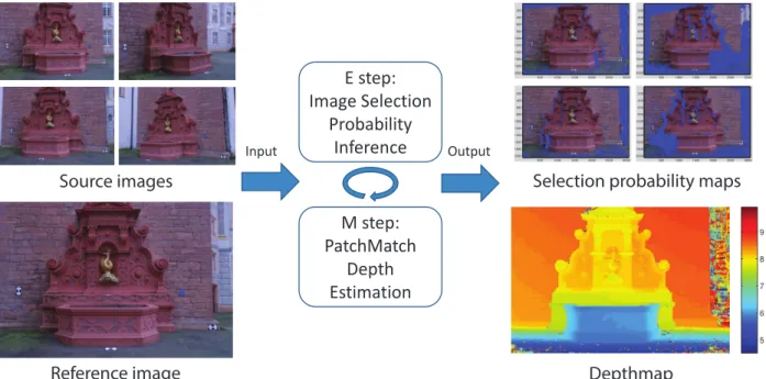
E step: Image Selection Probability Inference M step: PatchMatch Depth Estimation
Input Output 500 1000 1500 2000 2500 3000 200 400 600 800 1000 1200 1400 1600 1800 2000 500 1000 1500 2000 2500 3000 200 400 600 800 1000 1200 1400 1600 1800 2000
500 1000 1500 2000 2500 3000 200 400 600 800 1000 1200 1400 1600 1800 2000
500 1000 1500 2000 2500 3000 200 400 600 800 1000 1200 1400 1600 1800 2000 Source images Reference image
Selection probability maps
Depthmap
Figure 3.1: Overview of our approach. Input imagery is used to jointly estimate a depthmap and pixel level view associations. Blue regions in the view selection probability map indicate pixels in the reference image lacking reliable observations in the corresponding source image.
homogeneous texture). These technical challenges render multi-view depth hypothesis evaluation as a problem of robust model fitting, where a demarcation between inlier and outlier photoconsistency observations is required. We tackle this implicit data association problem by addressing the question: What aggregation subset of the source image set should be used to estimate the depth of a particular pixel in the reference image?
leads to modeling the depth estimation problem as a Markov chain where the unobserved states correspond to binary indicator variables for the selection probability of each source image.
We summarize the contributions and advantages of the framework as follows.
1. Accuracy:Mitigation of spurious data associations at the pixel level provides state-of-the-art accuracy results for single depthmap estimation.
2. Efficiency:Deployment of PatchMatch sampling and propagation enables reduced computa-tional burden as well as GPU implementation.
3. Scalability: Linear storage requirement with respect to the number of source images, as opposed to the exponential growth in the joint view selection and depth estimation model by Strecha et al. (2006), enables handling selection instances comprising hundreds of images.
3.2 Joint View Selection and Depth Estimation
In this section we provide an overview of our PatchMatch propagation scheme (Section 3.2.1), describe our probabilistic graphic model (Section 3.2.2), describe our variational inference approxi-mation to the model’s posterior probability (Section 3.2.3 and Section 3.2.4) and finalize describing our implementation (Section 3.2.5).
3.2.1 PatchMatch Propagation for Stereo
(i-1, j)
(i, j)
(i, j-1)
(i-1, j)
(i, j)
(i, j-1)
(i-1,j-1)
(i, j)
(i,j-1)
(i-1,j-1)
(i+1,j-1)
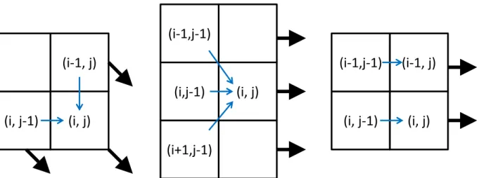
Figure 3.2: The black and blue arrows show the propagation directions and the sampling schemes. Left: Top left to bottom right propagation in (Bleyer et al., 2011). Middle: Rightward propagations in (Bailer et al., 2012). Right: Our rightward propagation.
In case of the absence of proper depth hypotheses, we can additionally draw and testHrandom depth hypotheses for each pixel during propagations. In this work, we useH = 1and hence have 3 depth hypotheses tested per pixel in a propagation, i.e. the depths of current and the neighboring pixel along with one random depth. Without loss of generality, we limit our discussion henceforth to the rightward horizontal propagation.
3.2.2 Graphical Model
In our algorithm, the depth is estimated for a reference imageXref, given a set ofM
(unstruc-tured) source images X1, X2, ...XM with known camera calibration parameters, which are the output of a typical structure from motion system such as VisualSFM (Wu, 2013). We denote the correct depth associated with each pixellon imageXref asθl.
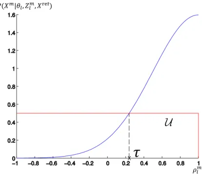
𝑃(𝑋𝑚|𝜃
𝑙, 𝑍𝑙𝑚, 𝑋ref)
𝜌𝑙𝑚
𝜏
Figure 3.3: Distribution of Equation (3.1)
reference imageXref, whereZm
l is 1 if imageXm is selected for depth estimation of pixell, and 0 otherwise.
We first define the likelihood function. We denote the color patch centered at pixell in the reference image asXlref. Given a pixelland its correct depthθlin the reference imageXref, a color patchXm
l on source imagemcan be determined through homography warping (Shen, 2013). If
Zm
l = 1, the probability that the observed color patchXlm is color-consistent withXlref should be high. We use NCC (normalized cross correlation) to compare the two color patchesXm
l andXlrefas a robust proxy to single pixel comparisons, and denote the NCC measurement asρm
l . In the case whenZlm = 0,Xlmhas arbitrary colors due to factors such as occlusion or calibration errors, so the probability of observingXlm is unrelated toXref
l and considered uniformly distributed. Therefore we propose the following likelihood function
P(Xlm|Zlm, θl, Xlref)=
1
N Ae
−(1−ρml )2
2σ2 ifZm
l =1
1
NU ifZ
m l =0,
where A equals to R−11exp{−(12−σρ2)2}dρ and N is a constant. Note that NCC value ranges in
[−1,1]and equals 1 with the best color consistency. Consistent with our intuition, a color patch
Xlm with high NCC valueρml has high probability P(Xlm|Zlm = 1, θl, Xlref). U is the uniform distribution in the range[−1,1]with probability density 0.5. Note that NCC computation is affine invariant and multiple pairs of color patches can generate the same NCC value. To simplify the analysis without affecting depthmap quality, Equation (3.1) assumes the number of color patches
Xm
l that can generate any specific NCC value is the same and equals toN. Since only the ratio
P(Xm
l |Zlm = 1, θl, Xlref)/P(Xlm|Zlm = 0, θl, Xlref)matters in the model inference discussed in Section 3.2.3 and Section 3.2.4, we can safely ignore the constantN in Equation (3.1).
In Equation (3.1)σ is the parameter determining the suitability of an image based on NCC measurementρml . As seen in Figure 3.3, a soft thresholdτ is determined byσ. Ifρml is larger than
τ, it is more likely that imagemis selected, and vice versa. SinceXlrefis observed for each pixel,
P(Xm
l |Zlm, θl, Xlref)is simply denoted asP(Xlm|Zlm, θl)in the rest of the paper.
The depths of nearby pixels are considered independent, while the pairwise smoothness is put on the nearby selection variables along the current propagation direction (Figure 3.4) through the transition probabilities:
P(Zlm|Zlm−1) = 1−γγ 1−γγ. (3.2)
Settingγclose to 1 encourages neighboring pixels to have similar selection preference for source imagesXm. To enable parallel computation, we only enforce pairwise constraint on the pixels of the same row in the horizontal propagations. Note Figure 3.4 only shows one row of selection variables for each of the source images.
𝑍
21𝑍
𝐿1𝑍
12𝑍
22
𝑍
𝐿−12𝑍
𝐿2𝑍
1𝑀𝑍
2𝑀𝑍
𝐿−1𝑀𝑍
𝐿𝑀𝑋
11𝑋
21
𝑋
𝐿−11𝑋
𝐿1𝑋
22𝑋
𝐿−12
𝑋
𝐿2𝑋
1𝑀𝑋
2𝑀
𝑋
𝐿−1𝑀𝑋
𝐿𝑀… …
𝜃
1𝜃
2𝜃
𝐿−1𝜃
𝐿𝑍
𝐿−11𝑍
11𝑋
12Figure 3.4: The graphical model. θlis the depth of pixell. Zlmis the selection of imagemat pixell.
Xlmis the observation (colors) on the source imagemgiven depthθl.
joint probability is
P(X,θ,Z) = M
Y
m=1
[P(Z1m) L
Y
l=2
P(Zlm|Zlm−1) L
Y
l=1
P(Xlm|Zlm, θl)] L
Y
l=1
P(θl), (3.3)
whereLis the number of pixels along the propagation direction of the reference image. We use an uninformative uniform distribution for priorP(Zm
1 )as well as depth priorP(θl)since we have no preference without observations. However, computingP(X)is intractable as it requires to sum over all possible values ofZandθ.
3.2.3 Variational Inference
Variational inference selects a member of a restrictedfamily of distributionsq(Z,θ)to ap-proximate the true posterior distributionP(Z,θ|X), in the sense that the KL divergence between these two is minimized (Bishop, 2006). The restriction is imposed purely to achieve tractability. The real posterior distribution is over the set of unobserved variables θ = {θl|l = 1, ..., L} and Z ={Zm|m= 1, ..., M}, whereZm ={Zm
1 , Z2m, ..., ZLm}is a chain in the graph. We put restric-tions on the family of distriburestric-tionsq(Z,θ), assuming that it is factorizable into a set of distributions (Bishop, 2006):
q(Z,θ) = YM
m=1qm(Z
m)YL
l=1ql(θl). (3.4)
For tractability, we further constrain each ql(θl),l = 1,2, ..., Lto the family of Kronecker delta functions:
ql(θl) = δ(θl =θ∗l) =
1, ifθl =θl∗ 0, otherwise
(3.5)
whereθ∗l is a parameter to be estimated. This assumption is in contrast to most other works (Strecha et al., 2004, 2006; Sun et al., 2002, 2005), which discretize the depth as a means to recover the whole posterior distribution of the depth. Once the distributionql(θl)is determined,θlis set toθl∗to maximize the approximate posterior distribution Equation (3.4), soθl∗is actually the final estimated depth. Conversely, the depthsθ can be considered as parameters shared by different chains instead of as variables. This assumption seamlessly combines the PatchMatch sampling scheme in the graphic model inference.
The variational method seeks to find a memberqopt(Z,θ)=QM
m=1q opt
m (Zm)
QL
l=1q opt
constrained to be a Kronecker delta function):
minimize
q(Z,θ) KL(q(Z,θ)||P(Z,θ|X))
subject to X
Zmqm(Z
m) = 1,m= 1, . . . , M.
(3.6)
Note the optimization is performed over distributions, but not over variables. To optimize over
qm(Zm), the standard solution (Bishop, 2006) islog (qm(Zm)) =E\m[log (P(X,θ,Z))] +const, whereE\mis the expectation oflog (P(X,θ,Z))taken over all variables not inqm(Zm)(Bishop, 2006). Then we have
qoptm(Zm)∝Ψ(Zm)YL
l=1P(X
m l |Z
m
l , θl =θ∗l), (3.7)
where Ψ(Zm)=P(Z1m)Ql=L
l=2 P(Z
m l |Z
m
l−1). The right side of Equation (3.7) has form of joint
probability of a Hidden Markov Chain with fixed transition probability from Equation (3.2) and fixed emission probability Equation (3.1). The probability of each hidden variableq(Zlm)can be efficiently inferred by forward-backward algorithm (Bishop, 2006). See Section 3.2.4 for more details. This corresponds to the E step of the GEM algorithm.
To optimize over ql(θl) we seek an optimal parameter θlopt for the distribution ql(θl) that minimizes Equation (3.6). Suppressing the terms not involvingθl gives
θoptl = argmax θ∗l
M
X
m=1
q(Zlm=1) lnP(Xlm|Zlm=1, θl=θl∗). (3.8)
By substituting Equation (3.1) into Equation (3.8), we get
θlopt =argmin θ∗l
XM
m=1q(Z
m
l = 1)(1−ρ m l )
2,
(3.9)
side of Equation (3.9) is a weighted sum of(1−ρm
l )2 with weight equal to the image selection probability. Hence, a small value ofq(Zm
l = 1), designating imagemas not favorable, contributes less in evaluating the parameterθ∗l.
Improvement: Equation (3.9) is computationally expensive for hundreds of source images.
Based on Equation (3.9), it is unnecessary to computeρm
l if the corresponding image selection probability q(Zlm = 1)is very small. Hence, we propose a Monte Carlo based approximation (Bishop, 2006). Rewriting Equation (3.9) as
θlopt =argmin θ∗l
XM
m=1P(m)(1−ρ
m l )
2 (3.10)
where the new distributionP(m) = q(Zlm=1)
PM
m=1q(Zlm=1)
can be deemed as the probability of image m
being the best for depth estimation of pixell. We draw samples based on the distributionP(m)to obtain a subsetS, then
θlopt =argmin θ∗
l
1 |S|
X
m∈S(1−ρ m
l )2. (3.11)
Empirically, 15 samples suffice to attain good results. Both distributionsqopt
m(Z)andq
opt
l (θl)are coupled. The computation ofθl∗ requiresq(Zlm)to be known (Equation (3.9)), but to inferq(Zlm)in Equation (3.7), we needθl∗available. The next subsection introduces the update scheme that computes the distributions iteratively.
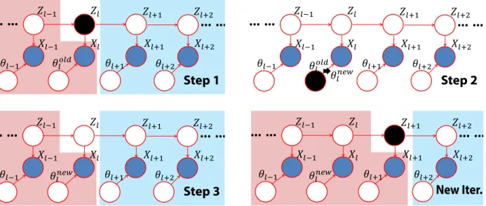
3.2.4 Update Schedule
Step 1
ܺିଵ ܺ ܺାଵ
ߠିଵ ߠௗ ߠାଵ ߠାଶ
ܼାଵ
ܼିଵ ܼ
ܺାଶ
ܼାଶ
… …
… …
ߠ௪ Step 2
ܺିଵ ܺ ܺାଵ
ߠିଵ ߠ௪ ߠାଵ ߠାଶ ܼାଵ ܼିଵ ܼ
ܺାଶ ܼାଶ
… …
… …
Step 3
ܺିଵ ܺ ܺାଵ ߠିଵ ߠ௪ ߠାଵ ߠାଶ
ܼାଵ ܼିଵ ܼ
ܺାଶ ܼାଶ
… …
… …
ܺିଵ ܺ ܺାଵ
ߠିଵ ߠௗ ߠାଵ ߠାଶ
ܼାଵ
ܼିଵ ܼ
ܺାଶ
ܼାଶ
… …
… …
New Iter. Step 1
Figure 3.5: Update schedule. See text for more details.
For more details on Hidden Markov Chain inference, we refer the reader to text (Bishop, 2006). The forward-backward algorithm is used to infer the probability of hidden variablesZl.
q(Zl) = 1
Aα(Zl)β(Zl), (3.12)
where A is the normalization factor. α(Zl)andβ(Zl)are the forward and backward message for variableZl computed using the following Equations,
α(Zl) = p(Xl|Zl, θl)
X
Zl−1
α(Zl−1)P(Zl|Zl−1), (3.13)
β(Zl) =
X
Zl+1
β(Zl+1)P(Xl+1|Zl+1, θl+1)P(Zl+1|Zl). (3.14)
Both the forward and backward messages are computed recursively (e.g.α(Zl)is computed using
α(Zl−1)). In Figure 3.5, the variables covered in red area and blue area contribute to the forward
and backward messages respectively.
We perform the following update schedule as is shown in Figure 3.5. In step 1, computeq(Zl) using Equation (3.12), (3.13) and (3.14) for each source image (i.e.q(Zm
Input: All images, depthMap (randomly initialized or from previous propagation)
Output: Updated depthMap
m– image index,l– pixel index
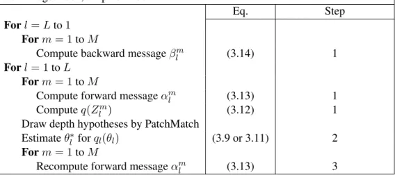
Eq. Step
Forl=Lto1 Form= 1toM
Compute backward messageβlm (3.14) 1
Forl= 1toL
Form= 1toM
Compute forward messageαml (3.13) 1
Computeq(Zlm) (3.12) 1
Draw depth hypotheses by PatchMatch
Estimateθ∗l forql(θl) (3.9 or 3.11) 2
Form= 1toM
Recompute forward messageαml (3.13) 3
Table 3.1: The algorithm of a row/column propagation.
we recompute forward messageα(Zl), which is further used to computeα(Zl+1)recursively in
Equation (3.13). Next we start at variableZl+1 with the same process until reaching the end of
the row in the image. Before the update process, the backward message for each variable can be computed recursively (Equation (3.14)) and stored in memory.
3.2.5 Algorithm Integration
leveraging GPUs. We describe the algorithm for processing one row within rightward propagation in Table 3.1.
Discussion. The estimation of the exact image-wide MAP for our graphical model would
require a Hidden Markov Random Field (MRF) formulation instead of our Hidden Markov Chain approximation. Our choice of using propagation direction specific chain models was driven by computational efficiency/tractability. The proposed framework enables us to easily interleave the propagation with hidden variable inference while fostering implementation parallelism. The enforcement of smoothness constraints on the hidden variables enables non-oscillating behavior of our evolving depth estimates. Our PatchMatch based framework has linear computational and storage complexity with respect to to input data size while being independent of the size of the depth search space. Namely, since the number of tested depth hypotheses (3 for each propagation) is small and constant, the computation complexity of our method isO(W HM), whereW,H, and
M are the width, height and number of images. Methods using complete hypotheses search, (e.g. Sun et al. (2002); Strecha et al. (2006)), requireO(W HM D)computations, where D is the size of hypotheses space normally reaching up to thousands of hypotheses.
3.3 Experiments
We evaluate the accuracy of our method on standard ground truth benchmarks and highlight our robustness on multiple crowd sourced datasets. In both evaluation scenarios we juxtapose our results with current state-of-the-art methods. We implemented our method in CUDA and executed on a Nvidia GTX-Titan GPU. For all experiments, the total number multi-directional propagations is set to 3 and we useσ = 0.45in the likelihood function (Equation (3.1)) andγ = 0.999in the transition probabilities (Equation (3.2)).
Ground truth evaluation. We evaluated on the Strecha datasets (Fountain-P11 and
2cm 10cm 2 cm 10cm
Error fountain-P11 Herzjesu-P9
Ours 0.732 0.911 0.619 0.833
Ours(P) 0.769 0.929 0.650 0.844
LC (Hu and Mordohai, 2012) 0.754 0.930 0.649 0.848 FUR (Furukawa and Ponce, 2010) 0.731 0.838 0.646 0.836 ZAH (Zaharescu et al., 2011) 0.712 0.832 0.220 0.501 TYL (Tylecek and Sara, 2010) 0.732 0.822 0.658 0.852 JAN (Jancosek and Pajdla, 2011) 0.824 0.973 0.739 0.923
Table 3.2: The percentage of pixels with absolute error less than 2cm and 10cm. EntriesOurs(P) andOursdenote our results with and without postprocessing. Reported values are from the work by Hu and Mordohai (2012).
depthmap instead of one consistent 3D scene model. We calculate the number of pixels with the depth error less than 2cm and 10cm from the ground truth and compare with (Hu and Mordohai, 2012; Furukawa and Ponce, 2010; Zaharescu et al., 2011; Tylecek and Sara, 2010; Jancosek and Pajdla, 2011). All the pixels with accessible ground truth depth are evaluated to convey both the accuracy and the completeness of the estimated depthmaps. We omit evaluation of the dataset’s two extremal views as done by Hu and Mordohai (2012).
We use slanted planes of single orientation instead of fronto-parallel planes. The single dominant orientation direction can be estimated by projecting sparse 3D points onto the ground plane as described in Gallup et al. (2007). We further apply two optional depthmap refinement schemes to increase the final accuracy. Our basic depth refinement uses a smaller NCC patch (5x5), while eliminating random depth sampling, during an additional propagation sweep. We then use deterministic fine-grain sampling (20 hypotheses) in the depth neighborhood (±1cm.) of each pixel’s depth estimate as proposed in Shen (2013). Finally, a median filter of size 9x9 is applied to each raw depthmap. Table 3.2 shows our method is comparable to the state-of-the-art methods. Note the results of Hu and Mordohai (2012); Tylecek and Sara (2010); Jancosek and Pajdla (2011) are obtained through multi-depthmap fusion, while our method directly estimates individual depthmaps.
Advantages of pixel level view selection. Figure 3.6 shows our comparison to the
1 2 3 4 5 6 7 8 9 10 0.6 0.62 0.64 0.66 0.68 0.7 0.72 0.74 0.76 0.78 0.8 K Accuracy Our (P)
Best K (10 source images) Best K (2 source images)
(b) (a) (a) (b) Ground truth (d) (d) (c) (c) (e) (e)
Figure 3.6: Left: Comparison against best-K aggregation. Right: Raw depthmap output of a partially occluded subregion with results for different dataset-aggregation combinations.
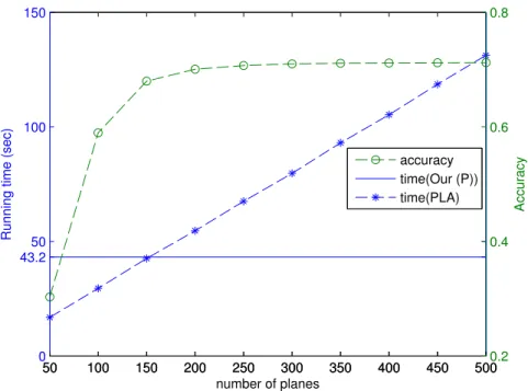
50 100 150 200 250 300 350 400 450 500
0 43.2 50 100 150
number of planes
Running time (sec)
50 100 150 200 250 300 350 400 450 5000.2 0.4 0.6 0.8 Accuracy accuracy time(Our (P)) time(PLA)
source images, it degenerates to the basic planesweeping algorithm that computes the cost using all source images. As opposed to our method with dynamic weights of images used for depth recovery, this method has a worse ability to handle occlusion. We compute depthmaps of the fountain-P11 data with varying K and otherwise fixed parameters, using 2000 planes. The percentage of pixels within 2cm difference from the ground truth is taken as a measure of the error. We run the planesweeping using two different dataset types. In the first case all 10 source images are used. Alternatively, we use the neighboring left and the right images. Figure 3.6 shows our results outperform all fixed aggregation schemes and illustrates the raw depthmap output of a partially occluded subregion.
Run times for our method are compared with an optimized GPU planesweeping code. Figure 3.7 shows the linear dependence of computation time to the number of planes as well the diminishing accuracy improvements provided by increasing the search space resolution. Our PatchMatch sampling and propagation scheme only requires depth range specification, foregoing explicit search space discretization.
Robustness to noisy SfM estimates. The advantage of pixel-level view selection across the
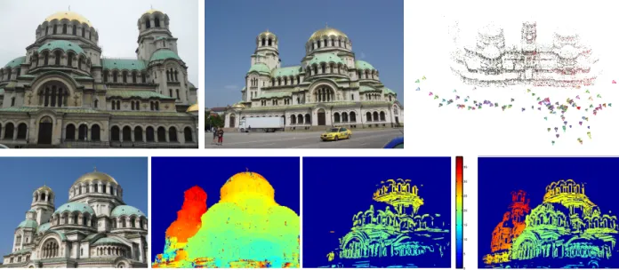
0 5 10 15 20 25 30 35
Figure 3.8: Top: Front and back of Alexander Nevsky Cathedral and estimated 3D model. Bottom: original image, depthmap of our method and the method by Goesele et al. (2007) with wrong and correct camera poses.
Robustness to varying capture characteristics. We tested our algorithm on Internet photo
collections (IPC) downloaded from the Flickr for six different scenes: Paris Triumphal Arch (195 images), Brandenburg Gate (300 images), Notre Dame de Paris (300 images), Great Buddha (212 images), Mt. Rushmore (206 images) and Berlin Cathedral (500 images). In order to control GPU memory, we optionally resize imagery to no more than 1024 pixels for each dimension. Camera poses were calculated using VisualSFM (Wu, 2013). The average run time for Berlin Cathedral is 98.3 secs/image. For illustration, sky region pixels are masked out using the method in Derek Hoiem (2005) as post-processing. To compare with the method by Goesele et al. (2007), we run the author’s code1 on the same dataset with default parameters except for setting the matching window size
to the same as ours (7x7). The results shown in Figure 3.9 illustrate that, while both approaches are robust to wide variations in illumination, scale and scene occlusions across the datasets, our approach tends to provide increased completeness of depthmap estimates. We attribute this to our more flexible view selection framework. In contrast to the method by Goesele et al. (2007), we avoid making initial hard image discriminations through an initial global image subset.
4 5 6 7 8 9 10 11 4 4.5 5 5.5 6 6.5 7 7.5 8 8.5 9 12.5 13 13.5 14 14.5 15 15.5 16 16.5 17 15 20 25 30 35 40 0 2 4 6 8 10 12 14 16 4 4.5 5 5.5 6 6.5 7 7.5 8 45 40 42 44 46 48 50 52 54 56 58 60 62 0 5 10 15 20 25 30 35 40 30 32 34 36 38 40 42 44 46 48 50 35 40 45 50 40 42 44 46 48 40 44 45 46 47 48 49 50 2 36 38 41 42 43 5 5.5 6 6.5 7 7.5 8 8.5 9 9.5 10 2.5 3 3.5 4 4.5 5 5.5 6 6.5 7 4 4.5 5 5.5 6 6.5 7 7.5 8 2 3 4 5 6 7 8
(b)
1 2 3 4 5 6 7 8 9 10 0.65
0.7 0.75 0.8 0.85 0.9 0.95 1
threshold (cm)
percentage of pixel
Our (P) GOS PLA
(b)
Figure 3.10: Fountain dataset performance.Percentage of pixels given different thresholds. PLA is the planesweep algorithm with all source images and K=3, while GOS is the method by Goesele et al. (2007).
To quantitatively compare the accuracy of our results with the work by Goesele et al. (2007), in the absence of ground truth geometry for crowd source datasets, we revisit the accuracy of both methods in the Strecha Fountain dataset. The method by Goesele et al. (2007) rejects outlier depth estimates based on the NCC values and the viewing angles. Hence, we only compare the accuracy of the reliable pixels as classified by Goesele et al. (2007) (comprising 75.4% of total image pixels). Figure 3.10 shows our approach outperforming both the method in Goesele et al. (2007) and planesweep for high accuracy thresholds. We expect the same accuracy ranking to carry over to the crowd sourced data results.
3.4 Conclusion
CHAPTER 4: JOINT OBJECT CLASS SEQUENCING AND TRAJECTORY TRIANGULATION (JOST)
4.1 Introduction
Techniques of 3D reconstruction from crowd-sourced imagery have developed rapidly over the past decade (Agarwal et al., 2011; Frahm et al., 2010; Zheng et al., 2014a; Heinly et al., 2015). Despite these advances, the state-of-the-art methods only target the static parts of a scene, treating the dynamic elements as hindrances to reconstruction. Since dynamic objects are typically the major focus of real-life images, recovering their 3D information enables applications such as better scene visualizations and dynamic event analysis. Therefore, it is of great interest to reconstruct these dynamic objects.
In this chapter, we propose a method to estimate the 3D positions of dynamic objects of the same class moving in a common path given a set of unstructured images as input. Figure 4.1a shows example input images in a dateset that captures pedestrians walking on a sidewalk. We assume no temporal correlation among the images, and that no two images observe the same dynamic object instance. The main challenge of the reconstruction problem resides in recovering 3D positions given noncurrent captures (or even single observations) of the dynamic objects, which invalidates the use of traditional 3D triangulation. The only constraint available for our problem is the fact that all observed instances of an object class move along a possibly diverging path in the 3D scene, which we define as an object class trajectory. Figure 4.2 shows one example of object class trajectory.
(a) (b)
Figure 4.1: Left: Tree images of the pedestrian dataset and the output of structure from motion. Right: Estimated 3D positions of two pedestrians that are captured in the image. Note we only reconstruct one 3D position for each dynamic object instance instead of a dense 3D model. For visualization purposes, a general mesh model is inserted into each estimated position.
To recover the object class trajectory, our method simultaneously determines the sequencing information of the objects and their 3D positions on the path, which we call joint object class sequencing and trajectory triangulation (JOST). We leverage all the observations on different images to recover the object class trajectory, which in turn provides an estimate for the 3D positions of the dynamic objects in each image (see Figure 4.1b).
4.2 Joint Object Class Sequencing and Trajectory Triangulation
We now detail our method for joint object class sequencing and trajectory triangulation from unstructured images. Our method includes three steps:
1. Spatially register the cameras to a common 3D coordinate system using structure from motion (SfM).
2. Detect object instances and estimate motion tangents from input imagery as the 2D observa-tions of the dynamic objects.
3. Leverage the observations of the object instances to simultaneously
(a) determine the sequencing information of the objects along a trajectory (i.e., the topology of the trajectory), and
(b) triangulate the geometry of the corresponding object class trajectory.
While we exploit known methods to solve for camera registration, object detection, and motion tangents in the images, our main contribution is an algorithm for tackling challenge 3. To this end, we model our problem as a nonconvex optimization problem, and develop a novel solver involving a step of discrete optimization followed by another step of continuous refinement. Next, we introduce our system in detail.
4.2.1 Spatial Registration
static background structures, we use the publicly available structure from motion tool VisualSFM (Wu, 2013) to register all the cameras. See Figure 4.1a for an example.
The obtained camera registration determines the camera centerC˜j of thej-th camera. With known camera parameters, each pixel in a camera defines a viewing ray with directionrin the 3D scene space. For our object class trajectory, we are only interested in the ray directionriassociated with the object instanceiof the desired class (for simplicity we refer to them as objects), where
i= 1, . . . , N, andN is the total number of detected objects over all frames. The rayXi(ti)in the 3D space represents a 1D subspace on which the imaged object has to lie and is described by
Xi(ti) =Ci+tiri, (4.1)
where ti ≥ 0 is the positive distance from the camera center Ci along the ray Xi(ti). In the following, we implicitly assume the conditionti ≥0. We denote the camera center associated with an object instanceiasCi withCi =C˜j, whereC˜j is the center of the cameraj in which the object instanceiis detected. This means if more than one object is detected in cameraj, there will be multipleCi with identical positions. Once we obtain the value forti, the object position can be uniquely determined.
4.2.2 Object Detection and Motion Tangent Estimation
Our proposed method leverages object detection techniques to determine the 2D observations of the dynamic objects. We identify one 2D position of each detected object on the image by the center of the detection bounding box. These object detections provide us the viewing rays where the dynamic objects are placed.
videos (Zhao et al., 2003), but in the absence of temporal coherence among the images, our method needs to estimate the motion tangent based on a single image.
The particular choice of object detection and motion tangent estimation methods depends on the specific object class and the scenes. We discuss our choices in Section 4.3, and for now we assume we have at our disposal the 2D observation defining the ray Xi(ti), as well as a coarse estimate of the motion tangentdifor each objecti.
4.2.3 Object Class Trajectory Triangulation
Assuming known viewing raysXi(ti)and the motion tangent di, we now define the object class trajectory estimation problem before delving into our data representation and our estimation framework. For ease of description, we directly leverage the viewing raysXi(ti)of the detected objectsiand thereby implicitly use the camera parameters and the 2D observations.
For a particular class of objects, an object class trajectory describes a path taken by the dynamic objects of the desired class through the 3D scene. Each observation (object detection) is a sample of the point on the trajectory. Since there are only a finite number of observations of objects along the path, we only sample a discrete set of 3D points on the path, and the combination of piecewise linear functions between the true object positionsX∗i represents the object class trajectory.
An important principle for obtaining an object class trajectory is that sampling along a path results in a collection of spatially adjacent points. A trajectory should therefore connect all observed points in such a way that total (spatial) traversal between the points is minimized. We formulate this as a minimization of the following cost function:
min p
X
(i,j)∈p
kX∗i −X∗jk22. (4.2)
here p defines the topology spanning the path with minimum cost, given as a list of adjacency relationships between all the pointsX∗i,i= 1, . . . , N.
position of each objectialong its viewing rayXi(ti). We propose to find the adjacency relation by optimizing over variablest= [t1, . . . , tN]andpjointly as
min p,t
X
(i,j)∈p
kXi(ti)−Xj(tj)k22. (4.3)
To robustly recover both tand psimultaneously, we further leverage the information of motion tangent. The direction of the local trajectory should be the same or similar to the motion tangent of the dynamic objects. Given the motion tangentsdiestimated from the images, we can further constrain the trajectory, obtaining an optimization problem:
min p,t
X
(i,j)∈p
kdi,j×(Xi(ti)−Xj(tj))k22+λkXi(ti)−Xj(tj)k22, (4.4)
where the operator×is the vector cross product, andλis a positive weight (discussed at length in Section 4.2.7). The directiondi,j is selected fromdi anddj as the motion tangent that is closest to the 3D motion directionXi(ti)−Xj(tj). More details about computation ofdi,jwill be illustrated in Section 4.2.6. The first cost term in Equation (4.4) adds the penalization if the local direction of the recovered trajectory deviates from the motion tangent. The optimization procedure simultaneously determines both the adjacencypand the object positions throught.
Optimization of the non-convex function in Equation (4.4) is inherently difficult. To achieve this, we propose a new discrete-continuous optimization strategy using a generalized minimum spanning tree (GMST).
4.2.4 Generalized Trajectory Graph