PROJECTING WILDFIRE EMISSIONS AND THEIR AIR QUALITY IMPACTS IN THE SOUTHEASTERN U.S. FROM 2010 TO MID-CENTURY
Uma Shankar
A dissertation submitted to the faculty at the University of North Carolina at Chapel Hill in partial fulfillment of the requirements for the degree of Doctor of Philosophy in the Department
of Environmental Sciences and Engineering in the Gillings School of Global Public Health.
Chapel Hill 2019
Approved by: William Vizuete Francis S. Binkowski David Leith
© 2019 Uma Shankar
ABSTRACT
Uma Shankar: Projecting Wildfire Emissions and Their Air Quality Impacts in the Southeastern U. S. from 2010 to Mid-century
(Under the direction of William Vizuete)
Wildfires can severely impair the health of ecosystems, life forms and regional economies. In the rapidly changing U. S. Southeast, both climate and socioeconomic factors (e.g., population and income) drive wildfires, and need to be represented in wildfire inventories to assess the air quality (AQ) impacts and health risks of wildfires long-term. This motivated the development of a wildfire emissions projection methodology leveraging published models of annual areas burned (AAB) based on county-level socioeconomic and climate projections for 2011-2060. It is applied to project two sets of AAB with different climate downscaling approaches, to estimate wildfire emissions for 2010 and four mid-century years. These are compared with emissions estimated using 18-year historical mean AAB without changes in climate and socioeconomics. Competing climate and socioeconomic factors result in 7% - 32% lower projected AAB than historical values, and 13% - 62% lower fine particulate matter (PM2.5) emissions than estimated from historical AAB in the selected years, with climate driving their temporal variability.
Evaluation of the emissions projection methods in air quality (AQ) simulations against those using the National Emissions Inventory (NEI), and network observations for 2010 show little difference among the methods in ozone (0.08% - 0.93%) and PM2.5 (1% - 8%). Larger,
projection methods predict primary wildfire PM better than the NEI, providing confidence that they can assess current wildfire AQ impacts, while enabling longer-term AQ assessments unachievable with static inventories.
AQ simulations using the projected wildfire emissions, and projected emission reductions in SOx and NOx from energy and transportation (by ~80% at mid-century) show peak periods and locations of wildfire impacts on ozone and PM shifting from autumn in Midwestern locations in 2010, to warmer and drier summers east and south by mid-century, following the AAB
In loving memory of my parents, Madhuram and K. V. Shankar, and my brother-in-law V. S. Mahesh, my examples in courage and joyful dedication to work.
ACKNOWLEDGMENTS
My deepest thanks go to my beloved family, including my family of friends, for their unwavering support and encouragement. I am most grateful to my friend Dr. Suzanne Elizabeth “Zz” Szabo (1951 – 2012), but for whose material support in the last two years, this work could not have been completed.
I owe thanks to many mentors: Dr. Frank Binkowski, for launching and nurturing my career; my advisor Dr. Will Vizuete, for his endless patience, critical review and advice on this work; my other committee members Dr. Jason West and Dr. David Leith, for their guidance on these analyses, and Dr. Jeff Prestemon, for inviting me into his research, and funding this work; Dr. Doug Fox, my first mentor and co-PI in wildfire research; Dr. Don McKenzie, fire science guru, for his guidance on the fire modeling approach, his excellent writing skills and good humor; and Dr. Adel Hanna, and colleagues and co-authors at the University of North Carolina– Institute for the Environment for many years of collaboration and support. I am indebted to my former colleague Jeanne Eichinger, whose extraordinary skills in technical editing have
improved me as a writer. Special thanks to my former colleague Dr. Mohammed “MO” Omary, for his critical contributions to the emissions processing in this work. MO, this is for you!
TABLE OF CONTENTS
LIST OF TABLES ... xi
LIST OF FIGURES ... xiii
LIST OF ABBREVIATIONS ... xix
CHAPTER 1: INTRODUCTION ... 1
Assessing the Impacts of Wildfire on Future Air Quality: Rationale ... 1
Research Goal, Hypotheses, and Objectives ... 3
Background ... 3
Research Goal ... 5
Research Hypotheses ... 5
Objectives ... 6
CHAPTER 2: PROJECTING WILDFIRE EMISSIONS OVER THE SOUTHEASTERN UNITED STATES TO MID-CENTURY ... 9
Introduction ... 9
Methods... 14
Annual area burned estimation ... 15
Fire Scenario Builder ... 20
Results ... 23
Comparisons of AAB estimation methods ... 24
PM2.5 predictions from wildfires ... 27
Discussion ... 30
Conclusions and Future Work ... 34
Acknowledgments... 36
CHAPTER 3: EVALUATING WILDFIRE EMISSIONS PROJECTION METHODS IN COMPARISONS OF SIMULATED AND OBSERVED AIR QUALITY ... 50
Introduction ... 50
Methods... 55
Emissions Inventories ... 56
Air Quality Simulations ... 58
Observational Networks... 59
Model Evaluation Tools and Data ... 59
Results ... 60
Ozone ... 60
PM2.5 ... 69
Conclusions ... 82
Acknowledgments... 87
Methods... 122
Emissions inputs ... 122
Meteorological inputs ... 124
Other simulation inputs ... 124
Air-quality simulations ... 124
Analysis tools and data ... 125
Results ... 125
Hourly ozone over the fire season ... 125
Hourly ozone seasonal variability ... 127
Ozone time series ... 127
Ozone impact of wildfire emissions ... 128
PM2.5 over the fire season... 130
PM2.5 seasonal trends ... 130
PM2.5 impacts of wildfire emissions... 131
PM2.5 compositional variability ... 132
Discussion ... 134
Ozone projections ... 134
PM projections ... 136
Conclusions ... 138
CHAPTER 5: CONCLUSIONS ... 163
Introduction ... 163
Study 1 ... 163
Study 2 ... 164
Study 3 ... 167
General Conclusions ... 169
LIST OF TABLES
Table 2.1. Annual area burned data used in the wildfire inventories for the south-
eastern US ... 37 Table 2.2. WRF model physics options for the D01 and D02 modeling domains ... 38 Table 3.1. Summary of cases simulated in modeling study ... 88 Table 3.2. Ozone at selected locations from statistical d-s, dynamical d-s and AQS
network observations ... 89 Table 3.3. PM2.5 at selected locations from statistical d-s, dynamical d-s and the
IMPROVE network ... 90 Table 3.S1. Model performance statistics for monthly-averaged ozone vs. AQS
observations ... 101 Table 3.S2. Model performance statistics for monthly-averaged total PM2.5 vs.
IMPROVE observations ... 102 Table 3.S3. Model performance statistics for monthly-averaged sulfate (SO4) vs.
IMPROVE observations ... 103 Table 3.S4. Model performance statistics for monthly-averaged ammonium (NH4) vs.
IMPROVE observations ... 104 Table 3.S5. Model performance statistics for monthly-averaged nitrate (NO3) vs.
IMPROVE observations ... 105 Table 4.1. Seasonal mean and maximum differences in hourly O3 between wildfire
emissions methods in each modeled year. ... 140 Table 4.2. Locations and times of seasonal maximum differences in hourly O3 between
wildfire emissions methods in each modeled year. ... 140 Table 4.3. Domain-wide maxima and locations of the seasonal average impacts of wildfire
emissions on hourly ozone (ppbV) projected by the statistical d-s method. ... 144 Table 4.4. Seasonal mean and maximum differences in daily-average PM2.5 between wildfire
Table 4.5. Locations and times of seasonal maximum differences in daily-average PM2.5
between wildfire emissions methods in each modeled year. ... 144 Table 4.6. Domain-wide maxima and locations of the seasonal average impacts of wildfire
emissions on hourly PM2.5 (µg m-3) projected by the statistical d-s method. ... 144 Table 4.7. Difference (%) between statistical d-s and dynamical d-s in PM2.5 and
constituents by season and year. ... 145 Table 4.S1. Emission growth /control factors for pollutant emissions by anthropogenic
source sector used in the Sparse Matrix Operator Kernel Emissions (SMOKE)
processing system for the future-year simulations. ... 156 Table 4.S2. Monthly mean values and differences in hourly O3 in the months and
LIST OF FIGURES
Figure 1.1. From McKenzie et al. (2014) (Fig. 3). Master flowchart for a modeling system to predict the smoke consequences of changing fire regimes in a warming
climate. RCPs: Representative Concentration Pathways; GHG: Greenhouse gases. ...8 Figure 2.1. Flow diagram of various models and data needed for estimating benchmark
(2010) and future wildfire emissions. AAB, annual area burned; FWIs, fire weather
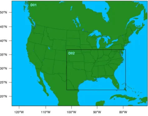
indices. ... 39 Figure 2.2. Modeling domains: D01 at 50-km x 50-km grid spacing; D02 at 12-km x
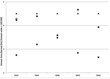
12-km grid spacing. ... 40 Figure 2.3. Time slices of total annual area burned (AAB) domain-wide (105 ha) in
domain D02 of Figure 2.2: historical (triangles) – historical mean value for 1992-2010 replicated in all years; statistical d-s (squares) – estimated using statistically downscaled meteorology from the Canadian General Circulation Model, ver. 3.1 (CGCM3.1) and A2 scenario realization; dynamical d-s (diamonds) – estimated with dynamically downscaled meteorology from the Canadian General Circulation Model, ver. 3 (CGCM3) and A2 scenario realization; open circle – historical 2010-only data. ... 41 Figure 2.4. Spatial distribution of historical mean AAB (ha) for 1992-2010. ... 41 Figure 2.5. Annual area burned (AAB) differences (ha) in future years above the historical
mean of Figure 2.4 for (L) statistical d-s (i.e., statistical d-s - historical) and (R) dynamical d-s (i.e., dynamical d-s - historical): Row 1, 2010; Row 2, 2043; Row 3,
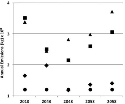
2048; Row 4, 2053; Row 5, 2058. ... 42 Figure 2.6. Time slices of annual domain-wide total wildfire PM2.5 emissions (108 kg) for
domain D02 of Figure 2.2 using historical (triangles), statistical d-s (squares) and dynamical d-s (diamonds) estimates of annual area burned (AAB). Shown for reference is the annual domain-wide total PM2.5 emissions level from point wildfires only in
the 2010 NEI (circles), replicated in all other years. ... 43 Figure 2.7. Spatial distribution of annual column total wildfire PM2.5 emissions (103 kg)
based on two AAB estimation methods: historical means (left panels) and dynamical d-s (right panels), for the future years: 1st row, 2043; 2nd row, 2048; 3rd row, 2053;
4th row, 2058. ... 44 Figure 2.8. Variability of seasonal domain-wide total wildfire PM2.5 emissions (106 kg) for
Figure 2.9. Spread of domain-wide AAB values around the annual mean for the AAB estimation methods in each of the modeled years: red: historical; green: statistical d-s; and blue: dynamical d-s. Note that the 2010 value for the historical mean
represents a multiyear average (1992-2010). ... 46 Figure 2.10. Precipitation and temperature differences between 2000 and 2060 decadal
averages for the conterminous US and the Southeast from nine downscaled climate models (L. Joyce, private communication; updated from Joyce et al. 2014). US data are represented by red squares and open diamonds, and the Southeast data, by black
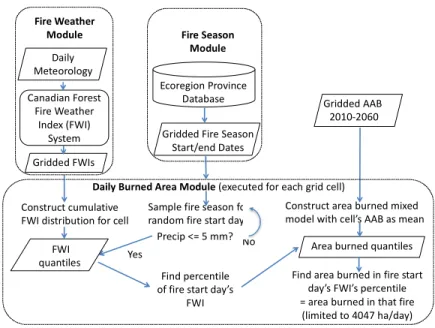
triangles and open circles. ... 46 Figure 2.S1. Schematic of the Fire Scenario Builder; FWI, Fire weather index; AAB,
annual area burned. ... 47 Figure 2.S2. Schematic of the Canadian Forest Fire Danger Rating System’s Fire Weather
Index System. Reproduced from Stavros et al. (2014). Numbers at the lower right corner of the modules denote the number of days that any given calculated index has an effect on subsequent calculated indices. (Note: T, temperature; P, pressure; RH, relative
humidity) ... 47 Figure 2.S3. From Prestemon et al., 2016 (Figure 4). Projections of all wildfires combined
for the south-eastern US in aggregate (i.e., sum of all areas burned for all counties in the region) for 2006, and 2010 – 2060, including upper and lower 90% bounds of 2250 Monte Carlo iterations of models under nine climate model realizations. Note: No
projections were made for 2005, 2007, 2008, or 2009. ... 48 Figure 2.S4. Spatial distribution of annual column total wildfire PM2.5 emissions (103 kg)
based on two annual area burned (AAB) estimation methods: historical means (left panels), and statistical d-s, (right panels) for the future years: 1st row, 2043; 2nd row, 2048; 3rd row, 2053; 4th row, 2058. ... 49 Figure 3.1. Modeling domains for the meteorological model: D01 at 50-km x 50-km grid
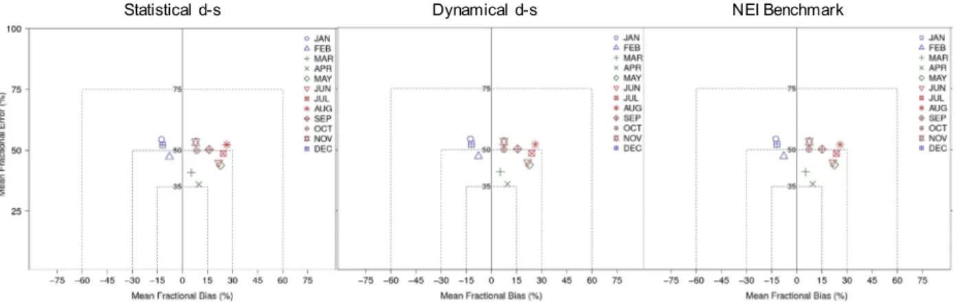
spacing; D02 at 12-km x 12-km grid spacing ... 91 Figure 3.2. Monthly average performance for 1-h ozone: mean fractional error (%) on the
vertical axis vs. mean fractional bias (%) relative to observations from the Air Quality System. L: statistical d-s; C: dynamical d-s; R: NEI benchmark. ... 92 Figure 3.3. Comparisons of wildfire emissions methods for 1-h O3 (ppb) predicted at grid
cells containing Air Quality System (AQS) monitors and wildfires in 2010. L: fire season (March – November); R: top and bottom, October; middle, July. The mean, maximum and minimum intermodel difference (vertical axis variable – horizontal axis variable), denoted, respectively, MeanDiff, MaxDiff and MinDiff, and the dates and
Figure 3.4. Seasonal comparisons of wildfire emissions methods for 1-h O3 (ppb) predicted at grid cells containing both Air Quality System (AQS) monitors and wildfires in 2010. The mean, maximum and minimum intermodel difference (vertical axis variable – horizontal axis variable), denoted, respectively, MeanDiff, MaxDiff and MinDiff,
and the dates and coordinates of their occurrence are shown in the plot legend. ... 94 Figure 3.5. Maximum absolute difference between statistical d-s and dynamical d-s in
each grid cell over the whole fire season in: Row 1, L – hourly VOC column emissions (g s-1); Row 1, R – hourly NOx column emissions (g s-1); Row 2 – hourly O3 mixing ratios (ppbV) in model layer 1. Here the fire season is defined as April 23 – November 30; almost all grid cell maxima in absolute difference in
hourly O3 occurred in this time period. ... 95 Figure 3.6. Monthly-averaged model performance for total PM2.5 and key wildfire
constituents relative to observations from the IMPROVE monitoring network.
Row 1, PM2.5; Row 2, elemental carbon (EC); Row 3, organic carbon (OC). ... 96 Figure 3.7. Domain-wide seasonally averaged total mass of PM2.5 (µg m-3) and fractional
mass of major constituents during the fire season compared to observations from the
IMPROVE monitoring network. ... 97 Figure 3.8. Comparisons of wildfire emissions methods for PM2.5 (µg m-3) predicted at
grid cells containing both Interagency Monitoring of PROtected Visual Environments (IMPROVE) monitors and wildfires in 2010. The mean, maximum and minimum intermodel difference (vertical axis variable – horizontal axis variable), denoted, respectively, MeanDiff, MaxDiff and MinDiff, and the dates and coordinates of their occurrence are shown in the plot legend. L: fire season (March – November); R: top
and middle, September; bottom – October. ... 98 Figure 3.9. Seasonal comparisons of wildfire emissions methods for PM2.5 (µg m-3)
predicted at grid cells containing Interagency Monitoring of PROtected Visual
Environments (IMPROVE) monitors and wildfires in 2010. The mean, maximum and minimum intermodel difference (vertical axis variable – horizontal axis variable), denoted, respectively, MeanDiff, MaxDiff and MinDiff, and the dates and
coordinates of their occurrence are shown in the plot legend. ... 99 Figure 3.S1. Spatial distribution of hourly ozone Mean Fractional Bias with respect to
AQS and SEARCH measurements in each season for each modeled case. ... 106 Figure 3.S2. Absolute difference between the statistical d-s and dynamical d-s cases in
1-h O3 mixing ratios (ppb) from Hour 0 - 23 (local standard time) for the 2010 fire
season (March 1 – November 30) over the whole domain (level 1). ... 107 Figure 3.S3. 1-h ozone mixing ratios (ppb) and bias (ppb) relative to AQS observations at
Figure 3.S4. Comparisons of wildfire emissions methods for maximum daily 8-h average (MDA8) O3 (ppb) predicted at grid cells containing Air Quality System (AQS) monitors and wildfires in 2010. Mean, maximum and minimum intermodel difference (vertical axis variable – horizontal axis variable), and the dates and coordinates of their occurrence are shown in the plot legend. L: fire season (March – November);
R: top, July; middle, September; bottom, October. ... 109 Figure 3.S5. Seasonal comparisons of wildfire emissions for maximum daily 8-h average
(MDA8) O3 (ppb) at grid cells containing both Air Quality System (AQS) monitors and wildfires in 2010. Mean, maximum and minimum intermodel difference (vertical axis variable – horizontal axis variable), and the dates and coordinates of their
occurrence are shown in the plot legend. ... 110 Figure 3.S6. Monthly-averaged model performance for inorganic PM constituents. Mean
fractional error (%) vs. mean fractional bias (%) relative to observations from the IMPROVE monitoring network for: Row 1, sulfate (SO4); Row 2, ammonium
(NH4); Row 3, nitrate (NO3). ... 112 Figure 3.S7. Monthly-averaged model performance comparisons for total PM2.5 between
the IMPROVE and CSN monitoring networks. ... 113 Figure 3.S8. Spatial distribution of total PM2.5 Mean Fractional Bias (MFB) with respect
to IMPROVE and CSN measurements in each season for each modeled case. ... 114 Figure 3.S9. Monthly-averaged model performance comparisons for PM constituents from
statistical d-s against multiple monitoring networks. Mean fractional error (%) vs. mean fractional bias (%) relative to observations. Row 1, organic carbon (OC);
Row 2, nitrate (NO3). ... 115 Figure 3.S10. Absolute difference between the statistical d-s and dynamical d-s cases in
PM2.5 concentrations (µg m-3) from Hour 0 - 23 (local standard time) for the 2010
fire season (March 1 – November 30) over the whole domain (level 1). ... 116 Figure 3.S11. Maximum absolute difference between statistical d-s and dynamical d-s in
each grid cell over the fire season in: L – hourly PM2.5 column emissions (g s-1), and R – hourly PM2.5 concentrations (µg m-3) in model layer 1. Here the fire season is defined as April 23 – November 30; almost all grid cell maxima in absolute hourly
PM2.5 concentration differences occurred in this time period. ... 117 Figure 4.1. Comparisons of wildfire emissions methods over the fire season for 1-hr O3
(ppb) predicted at grid cells containing Air Quality System (AQS) monitors and wildfires in each modeled year. The mean, maximum and minimum intermodel difference (statistical d-s – dynamical d-s), denoted, respectively, MeanDiff, MaxDiff and MinDiff, and the dates and coordinates of their occurrence are shown
Figure 4.2. Seasonal comparisons of wildfire emissions methods for 1-hr O3 (ppb) predicted at grid cells containing Air Quality System (AQS) monitors and wildfires
in each modeled year. The mean, maximum and minimum intermodel difference (statistical d-s – dynamical d-s), denoted, respectively, MeanDiff, MaxDiff and MinDiff, and
the dates and coordinates of their occurrence are shown in the plot legend. ... 147 Figure 4.3. Hourly ozone time series in the months and locations of maximum difference
in ozone (statistical d-s – dynamical d-s) identified in Table 4.2 over the fire season in each modeled year. Top: Chesterfield, MO, on the MO-IL border; Middle: L –
Moundsville, WV, near the WV-PA border; R – Middlesboro, KY, near the KY-TN
border; Bottom: L – Seabrook, TX, on the Gulf Coast; R – Middlesboro, KY. ... 148 Figure 4.4. Seasonal-average spatial distribution of hourly ozone mixing ratios (ppbV)
from a no-wildfire baseline simulation (Rows 1, 3 and 4) and difference in ozone (statistical d-s - baseline no-wildfire) simulations (Rows 2, 4, and 6) in each future year. Note the scale change in Row 6 to display the spatial pattern. Spr, Spring;
Sum, Summer; Aut, Autumn. ... 150 Figure 4.5. Comparisons of wildfire emissions methods over the fire season for PM2.5
(µg m-3) predicted at grid cells containing both Interagency Monitoring of PROtected Visual Environments (IMPROVE) monitors and wildfires in each modeled year. The mean, maximum and minimum intermodel difference (statistical d-s – dynamical d-s), denoted, respectively, MeanDiff, MaxDiff and MinDiff, and the dates and
Figure 4. 6. Seasonal-average hourly PM2.5 (µg m-3) from a no-wildfire baseline simulation (Rows 1, 3 and 4) and difference in PM2.5 (statistical d-s - baseline no-wildfire) simulations (Rows 2, 4, and 6) in each future year. Spr, Spring; Sum, Summer;
Aut, Autumn. ... 152 Figure 4.7. PM2.5 composition (µg m-3) averaged over IMPROVE sites in each season
in each modeled year from the dynamical d-s simulation (L) and the statistical d-s
simulation (R). ... 153 Figure 4.8. Seasonal average intermodel differences (statistical d-s – dynamical d-s) in
PM2.5 and constituents (µg m-3) in the years simulated. ... 153 Figure 4.9. Monthly total precipitation predicted by the WRF model in the summer months.
Row 1 – 5: 2010, 2043, 2048, 2053 and 2058; Row 6: October 2010 and August 2043, the months of maximum intermodel difference in ozone over the fire season in
those years. ... 154 Figure 4.10. Monthly average daily maximum temperature (°C) predicted by the WRF
model in in the summer months. Rows 1-5: 2010, 2043, 2048, 2053 and 2058; Row 6: October 2010 and July 2058, the months of maximum intermodel difference in both ozone and PM2.5 over the fire season in those years. The locations of their occurrence, also provided in Tables 4.2 and 4.4, are denoted by circles for ozone,
Figure 4.S1. Seasonal comparisons of wildfire emissions methods for PM2.5 (µg m-3) predicted at grid cells containing Interagency Monitoring for PROtected Visual Environments (IMPROVE) monitors and wildfires in each modeled year. The mean, maximum and minimum intermodel difference (statistical d-s – dynamical d-s), denoted, respectively, MeanDiff, MaxDiff and MinDiff, and the dates and
coordinates of their occurrence are shown in the plot legend. ... 158 Figure 4.S2. Seasonal-average concentrations (µg m-3) of PM2.5 and constituents over all
grid cells containing Interagency Monitoring for PROtected Visual Environments
(IMPROVE) monitors and wildfires in each modeled year from each modeled case. ... 159 Figure 4.S3. Potential evapotranspiration (PET – mm) used in the AAB estimates in July
of each future year, calculated from statistical downscaling (L), and dynamical
downscaling (R) of the meteorological inputs. ... 160 Figure 4.S4. Potential evapotranspiration (PET – mm) from statistical downscaling
averaged yearly in each of the modeled years. ... 161 Figure 4.S5. Monthly-averaged potential evapotranspiration (PET – mm) from
LIST OF ABBREVIATIONS
AAB Annual areas burned
AMET Atmospheric Model Evaluation Tool
AQ Air quality
AQS Air Quality System
AR3 Third Assessment Report (of the IPCC) AR5 Fifth Assessment Report
cb05tucl Carbon Bond 05 gas-phase mechanism with toluene and chlorine chemistry updates
CAP Criteria air pollutant
CSN Chemical Speciation Network
CFFDRS Canadian Forest Fire Danger Rating System CGCM3 Canadian General Circulation Model version 3 CGCM31 Canadian General Circulation Model version 3.1 CMAQ Community Multiscale Air Quality model CONUS Conterminous U. S.
EC Elemental carbon
EI Emissions inventory
EPA (U. S.) Environmental Protection Agency FCCS Fuel Characteristic Classification System FEPS Fire Emissions Processing System FSB Fire Scenario Builder
FWI Fire Weather Index
GHG Greenhouse gas
HadCM3 Hadley Centre Climate Model version 3
ICS 209 Incident Status Summary report by the National Interagency Fire Center IMPROVE Interagency Monitoring of PRotected Visual Environments
IPCC Intergovernmental Panel on Climate Change IVOCs Intermediate volatile organic compounds KBDI Keetch-Byram Drought Index
LBC Lateral boundary condition
LCC Lambert Conformal Conic map projection LSF Land surface feedback
MB Mean Bias
MCIP Meteorology-Chemistry Interface Processor
MDA8 maximum daily value of the 8-h running average of ozone MFB Mean Fractional Bias
MFE Mean Fractional Error
MODIS Moderate Resolution Imaging Spectroradiometer
NARCCAP North American Regional Climate Change Assessment Program NEI U. S. National Emissions Inventory
NMB Normalized Mean Bias NME Normalized Mean Error
NMVOC Non-methane volatile organic compound
NP National Park
NWR National Wildlife Refuge
PM Particulate Matter
PM2.5 PM below 2.5 µm in aerodynamic diameter POA Primary organic aerosol
RCP Representative Concentration Pathway
RCP4.5 RCP that stabilizes anthropogenic components of radiative forcing to 4.5 W m-2 by 2100
RCM Regional climate model RPA Resources Planning Act
RS Remote sensing
SEARCH Southeast Aerosol Research and Characterization
SMOKE Sparse Matrix Operator Kernel Emissions processing system SOA Secondary organic aerosol
SRS Southern Research Station, U. S. Forest Service SVOCs Semi-volatile organic compounds
VBS Volatility basis set
VOC Volatile organic compound
WRF Weather Research and Forecasting model
WRFG WRF with an improved scheme for convective parameters WSM6 WRF Single- Moment 6-Class microphysics scheme w/ graupel WUI Wildland-urban interface
CHAPTER 1: INTRODUCTION
Assessing the Impacts of Wildfire on Future Air Quality: Rationale
The adverse impacts of wildfires on the health of ecosystems, life forms and regional economies cannot be overstated. The loss of forested areas in catastrophic wildfires could increase their climate impacts through a reduction in the forest carbon sink depending on whether or not fire activity outpaces their ability to regenerate (Liu et al., 2011; King et al., 2012). Black carbon emitted in wildfires adds to the positive radiative forcing on climate, which was estimated to be as high as 1.1 W m-2 in a comprehensive review of the radiative impacts of black carbon (Bond et al., 2013). Climate change in turn has an impact on wildfires, due to an increase in conditions such as widespread drought coupled with warmer and drier weather patterns (Littell et al., 2010, 2016). These can increase the risk of fire recurring in the next wildfire season, particularly in the case of rainfall during the growing season that promotes new forest growth (Littell et al., 2010, 2016). Even when there is no further growth of vegetation to supply fuel for another fire, there is an increased risk of mudslides in sloping terrain denuded by fire, as happened in 2017 in the week following the Thomas Fire, one of the largest in California history; mudslides following wildfires resulted in 66 deaths in that year (Balch et al., 2018).
only on first responders (Wegesser et al., 2009), but on vulnerable populations exposed to the pollutant plumes in downwind areas (Fann et al., 2018; Rappold et al., 2011). These populations often lack the means for adequate protection measures and healthcare, adding to the wildfire health risks (Gaither et al., 2011). The extent of the wildland-urban interface (WUI) is increasing (USGCRP, 2018) alongside increasing wildfire, exacerbating the health risks of smoke exposure.
In this context, the economic costs associated with wildfires go far beyond those of fire suppression and recovery of values at risk. In a study of the health impacts of wildfires over the Northwestern and Southeastern U.S., Fann et al. (2018) estimated the economic impacts of wildfires in the form of additional premature deaths and hospital admissions between 2008 and 2012 in the range of $11B - $20B (2010$) per year, and far in excess of the cost of fire
suppression. Using data from the 2008 Evans Road Fire in eastern North Carolina, Rappold et al. (2014) estimated the economic benefits of avoided short-term healthcare costs through
interventions such as public health forecasts of smoke events to be a fraction ($1M) of the avoided long-term costs of additional mortality ($42M).
2017 wildfire season. Human-ignited fires are closely related to socioeconomic drivers such as population and income (Prestemon et al., 2013, 2016), especially in the Southeastern U.S., where humans both cause and suppress a majority of wildfires (Mercer and Prestemon, 2005;
Prestemon et al., 2013; Balch et al., 2017). As climate change is interconnected with changes in some of these socioeconomic drivers of wildfire, e.g., population and land use, integrated assessment methods that allow a simultaneous examination of their impacts on wildfires and downstream effects on ecosystems become even more important. Faced with fire activity patterns that are responding to evolving climate drivers as well as regional demographics, forest resource and air quality managers in the Southeast have a critical need to use such methods to develop effective plans for protecting the health and welfare of the public and the environment. The research described here is aimed at addressing this need.
Research Goal, Hypotheses, and Objectives
Background
SRS had previously developed statistical models (Prestemon and Butry, 2005; Mercer and Prestemon, 2005) to estimate AAB by broad cause (lightning- and human-ignited) to mid-century. These models were updated using inputs of monthly-averaged climate variables for temperature, precipitation, and fuel aridity from nine different climate realizations remapped to a column-row grid over the Southeastern U.S. at 12-km x 12-km resolution, with the goal of eventually using the AAB projections in air quality applications (Prestemon et al., 2016). In addition to the climate model inputs, the AAB projection models used socioeconomic inputs of income and population growth rates, and population density, projected over the Southeast from the 2010 county-level data to 2060 and beyond, under the same greenhouse gas (GHG) emission scenarios as were used in the climate realizations. These same GHG emission scenario
assumptions were also used to project county-level changes in the forest, cropland, pasture, and urban land use inputs to the AAB projections (Wear, 2013).
In addition to being used in long-term regional resource planning and land management, AAB projections such as these provide a critical input for estimating wildfire emissions that can be used to drive air quality simulations for long-term wildfire health risk assessments. However, current AAB projection methods lack the ability to allocate AAB to wildfire emissions even on monthly timescales. The need to bridge this gap to estimate wildfire emissions for assessing their future air quality impacts and health burden provides the impetus for this research.
Research Goal
The main goal of this research is to support effective land and air quality management practices in the coming decades in the Southeastern U.S. by developing reliable methods that include projected changes in the climate, socioeconomic and land use drivers of wildfires to estimate their emissions and assess their air quality impacts from the present to mid-century. The choice of the Southeast is not only motivated by changes evident in the climate system, but also by the rapid growth of this region, the expansion of the WUI, and the attendant increased access of populations to fuels as well as their increased risk of exposure to wildfire smoke.
Research Hypotheses
The following research hypotheses are tested in Chapters 2-4 of this dissertation.
Hypothesis 1: Expected changes in the climate and socioeconomic drivers of wildfires in the Southeast will cause wildfire emissions estimated with time-varying wildfire activity projection approaches to deviate significantly by mid-century from those estimated with (static) historical wildfire activity.
Hypothesis 3: Inclusion of climate and socioeconomic factors in the dynamic wildfire emissions estimation methods will result in considerably different ozone and PM2.5 spatial distributions and seasonal-average concentrations by mid-century from their 2010 levels. Objectives
The research hypotheses are tested by modeling wildfire emissions and air quality under scenarios for the Southeast that include projected changes in climate and socioeconomic factors from the present to mid-century, and by comparing those results with estimates of wildfire activity, emissions and air quality using static inventories based on historical or current data, and with observations for applicable periods. These studies address the following objectives:
1. Examine how wildfire emissions over the Southeast evolve relative to their historical levels under potential changes in climate and socioeconomic factors.
2. Evaluate how air quality predictions using the wildfire emissions projection methodology compare with those using benchmark (static) methods, and with observations when applied to a retrospective period.
3. Investigate the impacts of the projected wildfire emissions on air quality trends by mid-century relative to the retrospective period.
compared with emissions estimated using a static inventory based on 18-year historical mean AAB (1992-2010) that do not consider future changes in climate and socioeconomics. The second study (Chapter 3) evaluates the wildfire emissions projection methods by using their emissions estimates in AQ simulations of the criteria pollutants (ozone and particulate matter less than 2.5 µm in diameter, denoted PM2.5) for 2010. The simulation results are compared to those using the (empirical) U. S. National Emissions Inventory (NEI) for 2010 wildfires, and to available network observations for 2010 (Shankar et al., 2019). The third study in this
CHAPTER 2: PROJECTING WILDFIRE EMISSIONS OVER THE SOUTHEASTERN
UNITED STATES TO MID-CENTURY1
Introduction
Wildfires have serious consequences for human health due to the dramatic increase in the concentrations of pollutants of known toxicity emitted in wildfire smoke. There have been several studies (Wegesser et al., 2009; Rappold et al., 2011; Fann et al., 2013) on the adverse health impacts of wildfire-emitted particulate matter (PM) and ozone. Wegesser et al., (2009) found the inherent toxicity of PM from wildfires to be greater than equal doses of PM in ambient air. These researchers have also attributed the toxicity of PM collected from Alaska wildfire sites in their study, in part, to reactive metals as a major source of carbon-centered free radicals, following the findings of Leonard et al., (2000, 2007). Toxic polychlorinated dibenzodioxins and dibenzofurans, and aromatic compounds are also emitted from forest and grassland fires (Gullett et al., 2008). In addition to their adverse health impacts, wildfires can cause extensive damage to human communities and structures and threaten the integrity of some ecosystems that are
sensitive to disturbance. For example, in 2016, nearly $2 billion of federal funds were spent suppressing wildfires that totaled more than 2.2 million ha (5.5 million ac) on lands managed by
1 This chapter previously appeared as an article in the International Journal of Wildland Fire. The original citation is
the USDA Forest Service and the Department of the Interior (National Interagency Fire Center, 2017a). Of these, the overall South-wide costs in 2016 of wildfire suppression of more than 494,000 ha (1.22 million ac) burned were reported at $121 million (National Fire and Aviation Management, 2017). Wildfires in Smoky Mountain National Park, TN, alone caused up to $2 billion in damages by some estimates (National Park Service, 2017) in late November that year. These are not the only costs of wildfires, however. A large part of the economic impact of wildfires is due to the human health impacts of smoke exposure. Fann et al. (2018) estimate the present combined healthcare costs of mortality and morbidity due to exposure to
wildfire-attributable PM below 2.5 µm in aerodynamic diameter (termed PM2.5) to be $63 billion (2010$) for short-term exposures, and $495 billion for long-term exposures nationwide. Rappold et al. (2011, 2012, 2014) came to similar conclusions in their study of the health costs of a 45-day peat bog fire in 2008 at the Pocosin Lakes National Wildlife Refuge in rural North Carolina, which was ignited by lightning following a long drought. Rappold et al. (2014) put the costs of
emergency department visits during the fire due to excess asthma and congestive heart failure at over $1M, but their estimated costs of general health outcomes, predominantly premature mortality, were $48.4 M, far in excess of the medical costs to treat short-term health outcomes.
wildfires in this region are more strongly connected to human factors (Prestemon et al., 2002; Mercer and Prestemon, 2005; Syphard et al., 2017). Humans both ignite more fires in this region (Balch et al., 2017) and actively participate in their suppression (Prestemon et al., 2013). Half of the major wildfires in late 2016 in and around Gatlinburg, TN, were attributed to human causes, punctuating the role of humans on wildfire occurrence in this region. Human factors also play a role in wildfire impacts via the demographics and income levels of the exposed populations (Gaither et al., 2011; Rappold et al., 2011, 2014). Increased urbanization and expansion of the Wildland-Urban Interface (WUI) is only expected to increase in the South in the coming
decades, increasing the vulnerability of populations to wildfire smoke exposure. In their study of 37 regions across the continental US, Syphard et al., (2017) find wide geographical variability in both the fire-climate relationship, and the role of human presence in fire regimes; their study suggests a geographically complementary role for the two. Thus, region-specific methods of constructing wildfire emissions inventories that account for changes in both climate and societal factors are a critical need for better estimating how wildfire emissions and their air-quality impacts will change in the Southeast and managing wildfires and their associated health risks long-term.
Current wildfire-emissions inventories (EIs), like those used to provide high-resolution inputs (at 12-km x 12-km grid spacing or finer) required for air-quality simulations, are typically constructed from the most current data of fire activity and fuel loads selected for their
through the NOAA Hazard Mapping System (Ruminski et al., 2006) and reconciled with ground-based fire reports in the SMARTFIRE emissions processing system (Larkin et al., 2009). The EPA’s National Emissions Inventory (NEI), for example, includes a fire-emissions inventory that is updated yearly for its base-year air-quality assessments and forecasting applications using fire activity from the USDA Forest Service Situation Reports, MODIS fire counts from HMS, and fire perimeters from the Monitoring Trends in Burn Severity project (Eidenshink et al., 2007), all of which are processed in SMARTFIRE (Pouliot et al., 2012; Larkin et al., 2014). On-the-ground data that are reported by state and local agencies can also be included once every three years, during the NEI release.
Wildfire-emissions inventories used in global and regional air-quality modeling characterize the atmospheric loadings due to wildfire emissions of pollutants and their precursors under current conditions. Using these inventories in future-year wildfire impact assessments will be
wrong from the start (McKenzie et al., 2014) because they do not account for changes in climate, land use, population density, or income levels (which may affect emissions exposures—e.g., Rappold et al., 2012). All of these factors are regional drivers in initiating and sustaining
model simulation for the future modeling period. The results of McKenzie et al. (2006) showed that this stochastic method estimated area burned in a historical fire season (2003) over the Pacific Northwest to within 8% of actual burned areas. These estimations as such do not include the influences that future changes in population and income could have on wildfire activity. Such changes have been shown (Prestemon et al., 2002, 2016) to be important for the human factors dominating wildfire areas burned in the Southeast. Furthermore, these estimates were applied for a visibility assessment using the CALPUFF dispersion model, and were not designed for use in regional-scale grid-based air quality simulation models.
The statistical models developed by Prestemon et al. (2016) take into account the combined impacts of climate and socioeconomic factors on wildfire occurrence to estimate AAB at the county level. These multi-stage regression models of historical AABs over the Southeast were used to make multi-decadal projections of future AAB for the region, with fine-scale projections of future climate, socioeconomic factors and land use change as inputs. The statistical models were validated in each stage of their construction against out-of-sample historical observations to eliminate bias. These models of AAB thus provide a framework for the construction of wildfire EIs that allow air quality and exposure assessments to be based on an evolving landscape of natural and human factors influencing fire occurrence, and to project future air quality in the coming decades more realistically in response to potential changes in climate and society.
inventories that do account for these changes. Consequently, we suggest that historical AABs cannot be used to represent the impacts of projected changes in climate and society in the region over the next four decades adequately. Given the uncertainties in the climate change estimates, and the importance of human influences on south-eastern US wildfires, both present and future (Prestemon et al., 2016), realistic emissions inventories for the Southeast require an integrated method that accounts for expected changes in both climate and society. Model projections of changes in fire activity and fuel loads due to climate change, coupled with projections of human-caused wildfire, could lead to more effective land and wildfire management in a manner that reduces the adverse air-quality impacts of wildfires in future years (McKenzie et al., 2014; Prestemon et al., 2016). The research presented here proposes and tests such a methodology in the south-eastern US. This work is not intended to be an exhaustive study of climate and socioeconomic drivers of wildfires in the Southeast, but rather the description of a feasible, scientifically sound, and regionally relevant methodology of constructing wildfire emissions projections that include the impacts of those drivers, and how they might change in the future.
The emissions projection methodology developed in this work addresses the stochastic process of wildfires. Although prescribed burning accounts for more ignitions in the Southeast than wildfires, these are, by definition, planned fires that therefore need very different projection methodologies, e.g., incorporating demographic and socioeconomic factors explicitly rather than implicitly through the AABs, as is done here, as well as incorporating different criteria for selecting the burn days. We address these and related issues in the “Conclusions” section.
Methods
changes in climate and society over the five decades from 2010-2060. It describes our
application of the statistical AAB estimation model of Prestemon et al., (2016) and of the Fire Scenario Builder (FSB) model (McKenzie et al., 2006), which uses these AABs as constraints to estimate daily areas burned based on wildfire ignition probabilities. The daily burned areas are then used in the BlueSky fire emissions model (Larkin et al., 2009) to estimate daily wildfire emissions that are needed as inputs for future air-quality simulations. Figure 2.1 shows a
schematic of these various models and data flows in constructing a wildfire emissions inventory. Annual area burned estimation
To evaluate the effects of including changes in regional climate and socioeconomics on wildfire activity in the Southeast, our current- and future-year AAB estimates using two different climate downscaling methods are compared against a base case of AABs over the region with no projections of climate or societal influences. A summary of the three AAB estimation methods is provided in Table 2.1. These are (1) a base case of historical mean AABs at the county-level calculated with data from 1992 to 2010; (2) a case with AABs that were estimated with the published statistical model of Prestemon et al. (2016) using statistically downscaled
methods. As empirically accounted for in Prestemon et al. (2016), some counties and years of the 1992-2010 historical had potentially invalid observations of wildfire areas burned in the Short (2014) database (K.C. Short, private communication). Gap-filling of these invalid observations of historical data was done by replacing potentially invalid observations in the Short (2014) database with in-sample predictions of AAB generated with the statistical models of Prestemon et al. (2016). Gap-filling accounted for 35.1% of the observations in the region, 1992-2010. The county-level historical mean AABs were remapped using a GIS tool on a column-row grid at 12-km x 12-km grid spacing over the south-eastern US modeling domain (D02) shown in Figure 2.2 for the wildfire inventory development; their sum over this domain is estimated at 450 499 ha (Figure 2.3). The historical case is equivalent to a projection of future wildfires in the Southeast that ignores changes in climate and socioeconomic factors, and the 19-year historical mean of AAB (1992-2010) is used as its representative constant value, as shown in the time slices in Figure 2.3. For reference, the actual-year AAB for 2010 is also shown in the figure.
To compare against the historical case, two AAB projections were made that do account for changes in climate and socioeconomic factors. Both of them projected the statistical models of Prestemon et al. (2016) onto both 2010 and to future climatology. The first case, hereafter called “statistical d-s”, used monthly average values of daily maximum temperature, minimum
temperature and potential evapotranspiration (PET – Linacre, 1977), and monthly total
over the south-eastern US, to domain D02 (Figure 2.2) at 12-km x 12-km grid spacing, and aggregated to the required monthly values.
Other key inputs for the statistical model are income and population growth. Projections of these variables were based on three of the greenhouse gas (GHG) emission scenarios
(Nakicenovic and Steward, 2000) formulated by the Intergovernmental Panel on Climate Change (IPCC) in support of its Third Assessment Report (AR3), which were used in the nine climate realizations (3 GCMs x 3 GHG emission scenarios) reported in Prestemon et al. (2016). The emissions scenarios A1B, representing high economic growth and low population growth, A2, representing moderate economic growth and high population growth, and B2, representing moderate economic growth and low population growth, provided the basis for the income and population growth rates used by Prestemon et al. (2016) for the Southeast from the 2010 county-level data to 2060. Historical data needed for projecting population growth at the county county-level were obtained from the US Census Bureau (2012). Historical annual personal income data by county came from the US Bureau of Economic Analysis (2013a) and were converted to real values (in constant 2005 dollars) using the US gross domestic product deflator (US Bureau of Economic Analysis 2013b). Projections of population and income at 5-year increments for each scenario were obtained from the USDA Forest Service (2014), and linearly interpolated for the intervening years. Finally, inputs to the statistical model of changes in land use expected under the future climate scenarios, including those due to changes in the use of forest, cropland, pasture, and urban lands, were estimated at the county level by Wear (2013).
mechanistically linked to projections of economic and population growth. These internally consistent socioeconomic projections were also the basis for the county-level projections used by Prestemon et al. (2016) for income and population growth and by Wear (2013) for land uses, which provided the input variables known to be connected to wildfires in the Southeast. Updating those projections to be consistent with the RCPs would have required a complete revamp of these region-specific projection data, and was beyond the scope of their work.
The second AAB projection used dynamical, rather than statistical, downscaling of climate model results to provide the meteorological inputs to the AAB estimator, and is hereafter called “dynamical d-s”. Meteorological fields for this projection were simulated by a mesoscale
meteorological model, the Advanced Research Weather Research and Forecasting (WRF) model version 3.4.1 (Skamarock et al., 2008), forced by dynamically downscaled climate model inputs at its lateral boundaries. The dynamical d-s projection was motivated by the need to examine the effects of using consistent meteorological inputs throughout the inventory development,
beginning with the annual area burned projections, and continuing on to the daily wildfire emissions estimates, as they would also be used later in the hourly air quality impact
assessments. Dynamical, rather than statistical, downscaling has been the practice over the past few decades for generating meteorological inputs for air quality models, because it provides a complete and consistent framework of hourly, 3-D meteorological fields needed to process emissions from all the meteorologically-driven sectors (e.g., vegetation, dust, sea spray, fires) and drive the air quality simulations, at the spatiotemporal scales appropriate for tropospheric chemistry and transport of trace pollutants. It is, therefore, important to understand its
meteorological fields (minimum and maximum daily temperature, PET and precipitation) from WRF were aggregated to the temporal resolution (monthly) of the predictor variables in the statistical model. Due to its high computational cost, the dynamical downscaling for this
comparative study could be done only in selected years over the south-eastern US (domain D02 in Figure 2.2), whereas the statistical downscaling could be done for every year from 2010-2060.
The GCM realization used for the dynamical downscaling and comparison with the statistical d-s results was selected from the publicly available outputs in the North American Regional Climate Change Assessment Program (NARCCAP – Mearns et al., 2009) archive. Provided in this archive were GCM outputs that had been dynamically downscaled with WRF at km x 50-km horizontal resolution over the conterminous US (CONUS) domain D01 in Figure 2.2. We examined the NARCCAP archive for parent GCM/GHG scenario combinations that matched those used for the statistical downscaling from Joyce et al. (2014), finding only one, the
nested multi-domain simulation with D01. The nest-down feature eliminates the possibility of undesired feedbacks from inconsistent schemes between the two domains.
Wildfire emissions for the three cases were estimated for a historical year, 2010, for eventual use in air quality simulations that will be evaluated against ambient observations. Since no downscaled data were available for the 2020-2040 period in NARCCAP, the future fire
emissions were projected every five years beginning with an arbitrarily selected future year close to the beginning of the 2040-2060 period– in our case, 2043 – providing inventories for 2043, 2048, 2053 and 2058 (thus the data gap 2010-2043). The random year selection seems
reasonable in light of the interannual variability seen in the AAB projections of Prestemon et al. (2016), which nevertheless showed a small but significant increase in projected median AAB over the region, 2056-2060, relative to 2016-2020.
To ensure a robust comparison between the statistical and dynamical d-s methodologies, the AAB projections for statistical d-s were then redone in this work using only the downscaled inputs from the CGCM31/A2 climate model realization. The AABs presented here for the statistical d-s therefore differ somewhat from those published in Prestemon et al. (2016), who reported projected median and uncertainty bands of AABs calculated using all nine climate realizations, even though the underlying statistical models remain the same.
Fire Scenario Builder
key assumptions of the FSB are (a) that a fire event in a grid cell will only occur once in a fire season (assuming that fuels cannot return to the landscape within the season), and (b) that a fire season is entirely contained within the calendar year. Using mean AAB associated with some baseline climatology, which is usually historical but not necessarily, the FSB samples a fire-start day randomly from the fire season based on an assigned probability distribution of fire
likelihood. This is typically uniform unless informed by particular fire-start data. Here, we use our three estimates of mean AAB – historical, statistical d-s, and dynamical d-s – as baselines for the historical case and the two projections. Although changes in socioeconomic variables are not explicitly input to the FSB, it implicitly includes the response of wildfires to changes in
socioeconomic factors via the AAB projections. For each model grid cell, the FSB constructs a cumulative distribution of area burned with the AAB for that grid cell as the mean, using a mixed model that is a negative exponential up to the 95th percentile and a truncated Pareto distribution beyond that value. The beginning and end dates of the fire season appropriate for the Bailey ecoregion province (Bailey, 1995) allocated to each model grid cell are read from a national database maintained by the USDA Forest Service. Fires are further constrained to burn only if precipitation is less than 5 mm/day. If it is above that, another fire-start day is sampled.
al., 2014). It is computed from the dynamically downscaled daily meteorology for all selected years. We note that the use of this metric necessitated the use of dynamically downscaled meteorological data in all daily fire emissions estimates, even in the case where the AABs were estimated with statistically downscaled meteorological inputs, because the temporal aggregation (monthly) at which the statistical d-s inputs were available was too coarse to calculate daily FWI. Area burned on the randomly selected fire-start day for each case is calculated as the quantile from the cumulative distribution of AAB that corresponds to the quantile of the FWI from the climatology for that case matching that day’s FWI. Fires as treated by the FSB can burn up to 4047 ha (10 000 acres) per day; larger fires are modeled as multiday fires.
At first glance, the use of our 12-km x 12-km spatial resolution may seem too coarse for the FSB, but our selection of this resolution can be understood as follows. The FSB is really
simulating annual fire activity as a surrogate for real fire simulation. Actual fires do not burn contiguously for 144 km2 except in extreme events, but the coarse scale (relative to that of typical fires) of the FSB application for air quality modeling requires a stochastic representation of AAB, the relevant fire metric. Therefore, the area burned in a single year (“fire”) is simulated by the FSB, constrained probabilistically by the historical mean (or a future-year annual mean). Lumping all possible “fires” in a year into a single “event” would cause drastic information loss at the scale of fire-spread models, but at our coarser scale it is the only tractable way to represent AAB, and actually limits the error propagation that would ensue from attempts to partition burned area into individual “fires” (somewhere within a 12-km x 12-km grid cell).
BlueSky fire emissions model
statistical d-s, and dynamical d-s). The BlueSky model accomplishes this by using the gridded daily burned areas in conjunction with fuel load data available in the Fuel Characteristic Classification System (FCCS) database (McKenzie et al., 2007) to estimate daily fire emission rates. BlueSky is a highly modular framework that links state-of-the-science models of
meteorology, fuels consumption, and emissions, and provides flexibility in the data sources for fire activity and fuel load inputs. Fuels consumption in BlueSky is based on the CONSUME model version 3.0 (Ottmar et al., 2006), the default modeling option, which is an empirical model developed by the USDA Forest Service based on 106 different pre- and post-burn plots covering several vegetation types and fire conditions. Emissions are estimated as daily rates by a fire emissions module for CO, CO2, CH4 and PM2.5. In our application, BlueSky is used at the latitude-longitude location of each fire strictly for estimating total emission magnitudes of the various emitted species. The fire emissions estimated in BlueSky for the “fire” modeled by the FSB are processed in the SMOKE emissions processing system similarly to other point sources, which are vertically distributed in the air-quality model simulation in a later step (not presented here), using the plume-rise algorithm within that model.
Results
Comparisons of AAB estimation methods
The purpose of these analyses is to examine the sensitivity of the statistical model estimates of AABs to the downscaling method used to provide their meteorological inputs, since the AABs are used as constraints on the daily burned area estimates needed to calculate wildfire emissions. AABs from the historical mean over a 19-year period, 1992-2010 (inclusive), provide a
benchmark to compare against the modeled estimates of AABs using the downscaled climate inputs. These historical mean AABs summed over the domain D02 add up to 450 499 ha, shown as a constant value in Figure 2.3 for all years modeled. The spatial pattern of the historical mean AABs is shown in Figure 2.4. Prestemon et al. (2016) found that human-caused ignitions, whether accidental or intentional, dominate over lightning-caused ignitions in the peak locations shown in Figure 2.4. These occur in the Western part of the domain, in Oklahoma, Arkansas and Missouri, along the Gulf coast, in Florida, up the Southeast Coast, and in the Appalachian region. These are regions where there are both an abundance of fuels and ample human populations with access to those fuels.
The domain-total AAB estimate in 2048 is much lower than in the other modeled years for the case of statistically downscaled meteorology (Figure 2.3). This low estimate can be explained through the interannual variability of the AAB from 2010-2060 shown in supplemental Figure 2.S3. As previously noted, the years for our study were selected at an arbitrary interval of five years beginning at a randomly chosen 2043. In a random year such as 2048, there can be as much as ±50 000 ha difference from the domain-total mean AAB value. The statistical d-s AAB
actual AAB value for 2010, the deviation of its AABs projections from the historical mean is a clear consequence of the influences of climate and socioeconomic factors, each with its own variability.
The spatial differences in AAB for the statistical d-s case from the historical case (Figure 2.5, left panels) show that in 2010, the positive and negative differences are smaller than those in other years, and largely offset each other. In 2043, there are large negative differences (i.e., historical AABs are much greater than the statistical d-s estimates) in the ecoregion provinces to the north in northern Missouri, offset by a large positive difference in ecoprovinces in Florida and along the Gulf coast. In 2048, the positive differences in these coastal ecoprovinces are not large enough to offset the negative differences in the interior of the domain, and the domain-wide difference is a net negative, consistent with the time-slice plot in Figure 2.3. In 2053, the small net positive difference is due to the positive AAB differences in these coastal ecoregion
provinces and much of Texas, outweighing the negative differences in the interior of the domain. Finally, in 2058, the spatial pattern once again shows negative differences dominating over larger areas of the domain, and to a greater extent than in 2010, with little or no contribution from Texas. The net result overall is a negative difference, i.e., lower AAB values in the statistical d-s case than in the historical.
AAB estimates for the dynamical d-s case are significantly lower than in the other two cases in each of the five modeled years (Figure 2.3). The temporal variability in AAB is also quite different between the two downscaling methods, with the closest agreement in 2048 (a difference of 10 814 ha), and the greatest differences in 2053 and 2010 (182 591 ha and 148 249 ha,
2.5, left panels). The greatest negative differences are seen to occur along the Gulf coast and Eastern seaboard, while the portion of the domain west and northwest of Missouri is the main contributor to positive differences. These positive differences offset the negative differences across the domain significantly in 2048, consistent with the smallest domain-wide difference in all the years shown in Figure 2.3 between the historical and dynamical d-s AAB estimates. Similar spatial offsets of positive and negative differences occur to a lesser degree in 2043 and 2053, although the net result domain-wide in each of these years is still a negative difference (i.e., the historical AABs are greater than dynamical d-s estimates). Unlike the case of the statistical d-s, the Appalachian region in the right panels has a persistent large negative
difference, as do parts of the Gulf coast; these are also areas where the historical mean AABs had the largest values (see Figure 2.4). As both the downscaling methods used the same parent
climate model realization, these differences in the spatial patterns in Figure 2.5 are a result of the differences in the downscaling methods themselves.
The right panels of Figure 2.5 indicate that dynamical downscaling leads to much less wildfire activity in the Southeast, relative to the 19-year historical mean, while statistical downscaling preserves more of the large-scale circulation patterns in the region in the future decade and shows smaller differences from the historical fire activity. Liu et al. (2013) also found such spatial differences in their analyses of future wildfire activity in the dynamically downscaled results with the HRM3 regional climate model (RCM) compared to the HadCM3 climate model used in their previous analysis (Liu et al., 2010). Their study over North American regions used the Keetch-Byram Drought Index (KBDI – Keetch and Byram, 1968) as the
showed a warming overall in the 2041-2070 period over North America relative to the 1971-2000 period, there were pronounced differences in the locations of peak precipitation and temperature between the HRM3 and the HadGCM. It is worth noting that their 2013 results are at a coarser resolution (50-km x 50-km) for the various regions, and used a different GCM/RCM combination to calculate future climate change from the one used in our study (CGCM3/WRFG) over the Southeast. The HRM3 model that they used for their Southeast assessments had the smallest KBDI increase of all the RCMs in NARCCAP in the future decades in the Central Plains and Deep South, the region of our study. By comparison, the WRFG, used to provide boundary inputs for our Southeast WRF simulation, showed more mixed results, with a moderate KBDI increase from warming and drying in the Deep South, but a KBDI decrease in the Central Plains due to increased precipitation in the future. However, our WRF model results for the Southeast are from a nest-down simulation at a 12-km x 12-km spatial resolution from the dynamically downscaled WRFG model results in NARCCAP. Any biases, particularly in
precipitation, relative to the GCM will be propagated in the boundary inputs extracted from those results and input to our Southeast WRF simulations. Another major difference in our method from the Liu et al., (2013) study is that their study did not consider county-level socioeconomic factors, and used a different indicator of wildfire, the KBDI, from our fire weather metric (FWI) and would be expected to produce different results. We explain this further under “Discussion”. PM2.5 predictions from wildfires
the BlueSky fire emission model was mapped to the south-eastern US domain (D02) modeling grid using the Sparse Matrix Operator Kernel Emissions (SMOKE) processor (Houyoux et al., 2000, Baek and Seppanen, 2018), and the gridded daily emissions were vertically integrated and summed over the year in each grid column for each year modeled. Consistent with the AAB estimates from the three cases shown in Figure 2.3, the PM2.5 emissions estimates are highest for the historical case, followed by the cases using AABs estimated with statistically and
dynamically downscaled meteorology. The historical and statistical d-s total PM2.5 emission trends follow each other closely in 2010 and 2043, while the dynamical d-s trends are 50% and 20% lower in these years, and even lower in the later years, except for the maximum in 2048 leading to good agreement with a correspondingly low value mentioned previously in the statistical d-s case. The dynamical d-s estimates of PM2.5 emissions are also the closest of all three cases to the NEI 2010 emission levels from point wildfires, which are shown here for reference. There is slightly less variability in the time slices of wildfire PM2.5 emissions using the historical mean AABs than in the case using statistically downscaled meteorology. As the AAB estimates used to constrain the daily burned areas are constant for the historical case, this emissions variability can be attributed to the mesoscale model calculation of the daily FWI. The tendency of the WRF meteorology is to lower the daily wildfire activity, and therefore the emissions, and this is once again evident in these emissions estimates for the historical case, albeit to a far lesser degree than in the dynamical d-s case.
PM2.5 emissions for the historical (and statistical) case show greater spatial variability within a given year than for the dynamical d-s case and higher values in the interior Southeast due to the underlying higher wildfire activity in this case. Significant differences in the spatial distributions of emissions can be seen between the two cases in any year along the Southeast coastal areas, the Appalachian region, eastern Texas and Oklahoma, and Arkansas and Missouri. Of these, the states to the west (the southern part of ‘Central Plains’ in Liu et al., 2013, 2014) were part of the region where the NARCCAP model combination of CGCM3/WRFG tended to predict more seasonal precipitation in the future years (2041-2070), in both summer and winter, compared to the historical period (1970-2000). The remaining regions, which roughly map to the ‘Deep South’ of Liu et al., (2013, 2014), saw a decrease in precipitation in the summer in the future years, but this decrease was among the lowest for all the model combinations in the NARCCAP suite. These spatial differences in wildfire PM2.5 emissions distributions between the statistical and the dynamical d-s cases therefore suggest that precipitation increases have an overriding influence on emissions compared to the temperature increases seen in future years.
The spatial distributions of PM2.5 emissions in Figure 2.7 in each of the future years are generally consistent with the trends of annual total AABs shown in Figure 2.3. The much lower AABs in 2048 for the dynamical d-s case translate into smaller, albeit more numerous, wildfires with lower annual total PM2.5 emissions in Figure 2.7. The biggest spatial differences in 2048 relative to the historical case are seen to occur in Appalachia, North and Central Florida, in eastern Texas and Oklahoma, and around the Arkansas-Missouri state boundary.
cases show the impact of the AAB constraints imposed on the PM2.5 emission rates. Furthermore, the impact of the dynamically downscaled meteorology is seen in the seasonal variability of these emissions. Both the historical AABs and those from the dynamical d-s yield the lowest emissions of PM2.5 in the spring and the highest in the summer, while the NEI estimates for 2010 had the lowest emissions in the summer and higher PM2.5 emissions in both spring and fall. These seasonal plots indicate that the common feature among the historical and dynamical d-s cases, which is the WRF meteorology used to calculate daily FWI, dictates the seasonal variability in wildfire activity in any given year, as well as the variability among the modeled years in each season. In all years, there is also a consistently more pronounced summer high in PM2.5 emissions in the historical than in the dynamical d-s case due to its (constant) higher AAB values. The variability of PM2.5 emissions among the modeled years also somewhat reflects the AAB difference patterns shown in Figure 2.5.
Discussion
variability can also be seen in this work, in the frequency distributions of Figure 2.9 of domain-wide totals around the annual mean of the gridded AABs in each year for each of the estimation methods. Due to the wide range of the data, values of AAB below 10 ha are not shown so that the trends around the median values can be seen more clearly. The historical mean AABs used to represent 2010 have a higher median value than either of the other two estimation methods, consistent with the time slices shown in Figure 2.3. The statistical d-s AAB distributions have higher maxima than the dynamical d-s distributions in every year, even though their median values are slightly lower than for the dynamical d-s in 2048 and 2058. The higher statistical d-s AABs are also consistent with the domain-total AAB time slices for these two cases (Figure 2.3). The effects of competing climate and socioeconomic factors in the AABs for the statistical d-s are also clear in Figure 2.3: any biases due to the dynamically downscaled meteorological inputs are not applicable in these AABs. Those biases would therefore also have a smaller impact on the PM2.5 emissions in this case (Figure 2.6) than in the dynamical d-s case.
The WRF model used in the dynamical downscaling yields very different spatial patterns of AAB from the statistical d-s AAB estimates. The differences between the AABs estimated from statistical and dynamical d-s are a consequence of differences between the downscaling methods themselves, as they are both using the same climate model (CGCM3.1), as well as GHG,