Some assembly required: the structural evolution and mass assembly of galaxies at z<5

(1)

The following handle holds various files of this Leiden University dissertation:

http://hdl.handle.net/1887/61630

Author: Hill, A.

Title: Some assembly required: the structural evolution and mass assembly of galaxies at

z<5

(2)

Some Assembly Required:

The Structural Evolution and Mass Assembly

of Galaxies at

z

<

5 Proefschrift

ter verkrijging van

de graad van Doctor aan de Universiteit Leiden,

op gezag van de Rector Magnificus Prof. mr. C. J. J. M. Stolker, volgens besluit van het College voor Promoties

te verdedigen op woensdag 18 April 2018 klokke 15:00 uur

door Allison Hill

(3)

Promotiecommissie

Overige leden: Dr. K. Caputi (Groningen)

Prof. dr. P. van Dokkum (Yale) Dr. A. van der Wel (Ghent) Dr. J. Hodge

Prof. dr. J. Schaye Prof. dr. P. van der Werff Prof. dr. H. J. A. R¨ottgering

ISBN 978-94-028-1005-9

(4)

(5)

(6)

Chapter

1

Introduction

Understanding how galaxies grow and evolve is an important question whose relev-ance spans many sub-fields in astronomy and astrophysics. It is a massive under-taking, encompassing billions of years of time. Observationally one needs to ex-plain how the minuscule initial density perturbations seen in the almost uniform microwave background radiation echoing from the big bang, grow into the com-plex, and diverse structure of galaxies we see in our own cosmic backyard. This work attempts to explain a little bit of what occurs in-between.

(11)

1.1 The Birth of Extra-Galactic Astronomy

At the time of writing, the field of extra-galactic astronomy is fast approaching its 100th year (or perhaps it has already elapsed - as with all things, it depends on how you count). Prior to the early 20th century, whether or not the stars, gas and dust that made up our Milky Way galaxy was the extent of our universe was an issue of considerable debate.

For over a thousand years, nebulae, or ‘clouds’ had been observed in the night sky. These nebulae turned out to be a diversity of objects including stellar nurs-eries, stellar remnants, and galaxies, with nebulae referring to an observational class of objects which appeared ‘fuzzy’ on the night sky. Several renowned figures from history including the astronomer William Herschel, and the philosopher Im-manuel Kant had subscribed to the idea that some of these nebulae were not small clouds that were members of our ‘universe’, but instead were hugeisland universes existing outside our own.

However their extra-galactic nature remained hotly debated until Edwin Hubble surveyed variable Cepheid stars in two of these nebulae documented in the Messier catalogue, M31 and M33 (Hubble 1925). Using the tight period-luminosity rela-tion known to this class of stars, he was able to prove conclusively that these ‘nebulae’ were much too distant to be a tiny component of our own galaxy, and instead were a massive arrangement of stars and gas, and galaxies in their own right. It was a paradigm shift on the scale of when Tycho Brahe’s observations of planetary motion confirmed the Copernican heliocentric model - the observable universe had just become a lot bigger, and our proximity to the centre of it was once again displaced.

Since Hubble’s first foray beyond the confines of our Galaxy, our understanding of the physical scale of the universe continues to expand; an expansion which is both literal, and figurative in nature. In 1929, Hubble noted a linear relationship between a galaxy’s distance to us and it’s recession speed, implying that the uni-verse was getting bigger (Hubble 1929). The idea that the uniuni-verse was expanding set the stage for a radical new view of cosmology, one in which our universe had a beginning from which to expand from. This cosmology invariably leads to a uni-verse in which galaxies grown and evolve, which is a central tenant to the study of extra-galactic astronomy.

1.2 Tracing Galaxy Evolution Using Integrated

Properties

(12)

Tracing Galaxy Evolution Using Integrated Properties

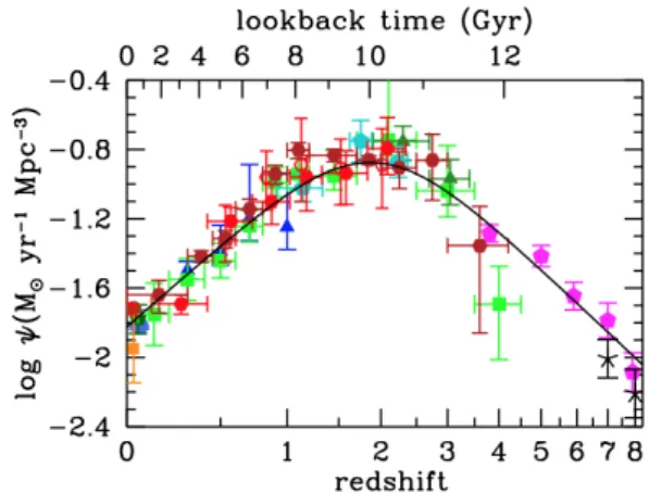
Fortunately, the invariability of the speed of light allows astronomers to ef-fectively look back in time by observing galaxies at greater and greater distances. Although we cannot observe the billion year evolution of a single galaxy in even a thousand human lifetimes, we can look at how properties of galaxies change at different redshifts and infer evolution. The most famous example of this method is the measurement of the integrated star formation rate (SFR) of all galaxies at different epochs (Fig 1.1). From Fig. 1.1, we are able to infer that galaxies were forming stars at a much higher rate than at the present day, and that this rate peaked∼10billion years ago.

Figure 1.1 The comic star-formation rate density across cosmic time from Madau & Dickinson (2014). Here we we see the peak of cosmic star formation occurred at z ∼ 2, or ∼ 10 Gyr ago. This tells us that galaxies were forming stars at a higher rate in the past and this has been on a steady decline continuing through the present day.

Although the cosmic star formation history is informative, it is an integrated property across all galaxies. It does not specify where star formation is concen-trated, in which galaxies most of the stellar mass is assembled, how the structure or morphology of galaxies change, the merger rates of galaxies, or whether these properties depend on stellar mass, dark-matter halo mass, gas fractions or any number of dependencies which might better explain the physics of what is driving evolution.

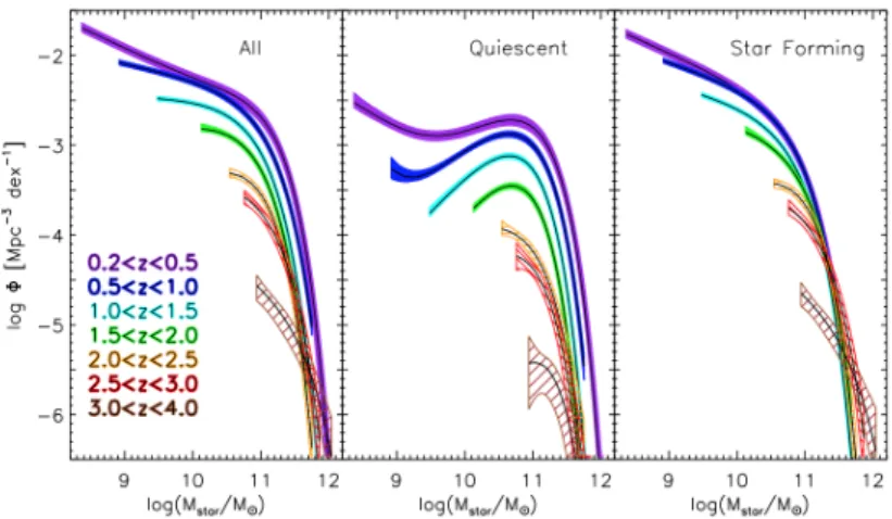
One way to achieve more specificity is to measure how the galaxy census evolves with redshift. In extra-galactic astronomy, the galaxy stellar mass func-tion (GSMF) provides the relative abundance of galaxies as a funcfunc-tion of mass in the form of number densities (e.g., Moustakas et al. 2013; Ilbert et al. 2013; Muzzin et al. 2013b). By measuring the GSMF at different redshifts, the changes in relative abundances can be determined (Fig. 1.2).

(13)

Figure 1.2 The evolution of the total (left), quiescent (centre) and star-forming (right) galaxy stellar mass functions from Muzzin et al. (2013b).

does not change significantly with redshift, suggesting these galaxies form at re-latively early times. Muzzin et al. (2013b) also separated the GSMF based on galaxies which are quiescent (i.e. not actively forming stars or are forming them at insignificant rates), and those that are actively star-forming. We see the corol-lary in the center and right panels of Fig. 1.2 - there is a decrease in the number density of the most massive star-forming galaxies, with a corresponding increase in the number density of the most massive quiescent galaxies. This suggests that the most massive galaxies were actively forming stars at high redshift, and have since quenched.

Together, the conclusions drawn from Fig. 1.1 and Fig. 1.2 are significant, and already reveal salient truths about how galaxies evolve. However, the questions posed earlier still remain unanswered. The GSMF obfuscates much of the specific evolution and does not explain the underlying processes that drive evolution. For instance - why do the most massive galaxies quench at high redshifts? Do they exhaust their gas reservoirs? Does feedback play a role? Is the feedback driven by star-formation, or from quasars? In order to answer these questions, it is necessary to develop a method to connect progenitors to descendants.

1.3 Progenitor Selection

The most straight-forward way to look at galaxy evolution as a function of stellar mass is to choose a fixed stellar mass, and see how galaxy properties change as a function of redshift (we have already implicitly done this with the example of the evolution in the GSMF from Fig. 1.2 and the discussion in Sec. 1.2 when we examined the change in number density of galaxies with a stellar mass of

(14)

The Structural Evolution of Galaxy Progenitors

galaxy evolves.

If we were to infer an evolutionary link from fixed-mass analysis, we have implicitly assumed that in almost 10 billion years of cosmic time galaxies do not merge, and that they form no new stars. From Fig. 1.1 we already know that the assumption that galaxies do not form new stars is an unreasonable one, and it has been shown that galaxies do in fact merge, necessitating alternative methods to connect progenitor to descendant.

There are many methods which have been used to select progenitors and draw direct evolutionary connections in the literature; via fixed central velocity dis-persion (e.g., Bezanson et al. 2012), the evolution of the SFR-stellar mass relation (e.g., Patel et al. 2013b), fixed central surface-mass density (e.g., van Dokkum et al. 2014; Williams et al. 2014) and more generally, number density arguments (e.g., Brammer et al. 2011; Papovich et al. 2011; van Dokkum et al. 2010, 2013; Muzzin et al. 2013a; Patel et al. 2013a; Marchesini et al. 2014; Ownsworth et al. 2014; Morishita et al. 2015). The required assumptions in some of the aforementioned methods are only applicable in specific regimes (i.e., massive elliptical galaxies, or field galaxies that have undergone no major merging). Since we wish to apply the method more generally, in this thesis we focus on number density selection arguments to choose progenitors.

The first example of using number density arguments to select progenitors was by van Dokkum et al. (2010), who used a constant number density to select the progenitors of today’s massive (∼1011.5M) galaxies out toz=2. By using a constant number density, van Dokkum et al. (2010) assumed that galaxies maintain rank order across cosmic time, that is, the most massive galaxy atz=2is still the most massive galaxy atz=0. This assumes that the two methods of mass growth, star formation, and merging, do not affect the number density across cosmic time. Mergers will certainly effect the number density, and the only way star formation will keep galaxies at the same rank order is if the specific star formation rate is independent of mass (which is not the case; Schreiber et al. 2015). One would expect the regime of validity of these assumptions to break down at flatter regions in the mass function (i.e., lower mass) as well as comparisons across large redshift ranges, where the errors associated with scatter in the mass accretion histories will begin to add up.

(15)

1.4 The Structural Evolution of Galaxy

Progen-itors

Using a constant number density selection, van Dokkum et al. (2010) investigated the structural and stellar mass evolution of the progenitors of today’s massive galaxies (1011.4_{) out to} _z ₌ _2. _{The authors traced the stellar-mass growth as}

well as the structural evolution using stacking analysis from galaxies in the NEW-FIRM survey, a NIR medium band survey designed to obtain accurate photometric redshifts from the rest-frame optical SED. From these stacks, surface brightness profiles were converted into surface mass density profiles to trace where mass was being accreted as a function of redshift. The most profound finding of this work was that the central regions in massive galaxies have undergone no appreciable mass evolution since z = 2, and all mass added has been in the outskirts, con-sistent with findings by other observationally driven studies (Hopkins et al. 2009; Bezanson et al. 2009). By comparing star-formation rates to the mass profile evolution, they conclude that star-formation was insufficient to explain the mass growth, and that minor mergers are the best candidate to explain the lack of self-similar growth between the interior regions and the outskirts; a viewpoint affirmed in subsequent studies (e.g., Hopkins et al. 2010; Trujillo et al. 2011; Newman et al. 2012; McLure et al. 2013; Hilz et al. 2013; Patel et al. 2013a). Sersic fits to the pro-genitor surface mass density profiles also show that the effective radius, and sersic index both decrease with increasing redshift, with a corresponding increase in the star-formation rate suggesting star-forming (and potentially disky) progenitors.

Using the abundance matching technique of Behroozi et al. (2013), Marchesini et al. (2014) re-visited the progenitors of massive galaxies. With a new selection, as well as the first data release of the deep, and wide (compared to surveys targeting similar redshift ranges, i.e. CANDELS) NIR UltraVISTA survey, Marchesini et al. (2014) targeted the more massive, and rarer ultra-massive galaxies (M∗∼1011.8). In addition to the corrected cumulative number density selection, the authors also used a constant cumulative number density selection as a comparison between the two techniques. As expected, the mass evolution for an abundance matched number density selection is steeper than a constant cumulative number density. This means the progenitors are less massive than would have been selected in previous works, with the mass differences greater than the uncertainties in the mass functions atz>2.

1.5 Galaxy Ages and Assembly Times

Arguably the most important ramification of the steeper mass evolution with red-shift found using abundance matching (as opposed to a constant cumulative num-ber density as discussed in the previous sections) is the effect this has on galaxy assembly times. If the progenitors at a given redshift are less massive than origin-ally thought, this implies that massive galaxies assemble their mass more quickly at later times. This results in a different ages of assembly for massive galaxies.

(16)

This Thesis

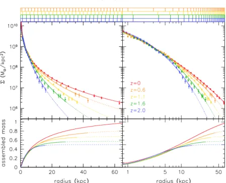
Figure 1.3 The stellar surface mass density profiles from van Dokkum et al. (2010) in linear (left) and log (right) units at redshifts spanning 0 <z < 2. From this figure, it is evident that massive galaxies grow more substantially at larger radii sincez=2.

the mechanisms involved in galaxy growth and evolution. Equipped with a reliable progenitor selection, the assembly time scales of galaxies can be gleaned by simple inferrence from the stellar mass evolution over time. Although constant cumulative number density over-predicts the assembly age, a comparison of the stellar mass evolution of a diverse mass range of descendants in Muzzin et al. (2013b) implies that massive galaxies have an earlier mass assembly than less massive galaxies (Fig. 1.4), and less massive galaxies have more rapid recent assembly.

(17)

Figure 1.4 Left: the average stellar mass evolution of galaxies with progenitors chosen at a constant cumulative number density which shows that massive galaxies assembled the bulk of their stellar mass at earlier times than less massive galaxies. Right: the derivative of the stellar mass evolution from the left hand plot as a function of redshift. Here we see that less massive galaxies show more rapid recent assembly. (Fig. 14 from Muzzin et al. (2013b))

1.6 This Thesis

As much work as has been done, there remain some open questions which this thesis addresses. van Dokkum et al. (2010) found that the surface mass density profiles of massive galaxies remain essentially unchanged sincez=2, which begs the question, when do the interiors assemble, and what do the progenitors of massive galaxies look like atz>2? Does the potential bias towards more massive progenitors in a fixed cumulative number density selection affect the median evolution in previous works? Does this bias also effect the inferred assembly times from Muzzin et al. (2013b)? We address these issues in Chapters 2 and 3.

The focus on the progenitors ofz=0massive galaxies in the literature is partly out of accessibility. Massive galaxies are host to the oldest stars, and also tend to be more luminous making them ideal candidates to trace out to higher redshifts. They are also large, and can be resolved to within 1reat higher-zthan lower mass galaxies. As such there is currently a dearth of information regarding the evolution of galaxies with M∗ <1011 at high-z z>2. We attempt to bridge this divide in Chapters 3, 4 and 5.

Chapter 2

(18)

This Thesis

masses are consistent within the uncertainties in the mass function. In accordance with previous trends, we find that the progenitors of massive galaxies have smaller effective radii, as well as smaller sersic indices. In contrast to previous findings, our progenitor selection shows stellar mass continues to be accreted at all radii at z< 2, although the build-up is more significant at larger radii. At z >4, we see evidence of significant mass growth in the central regions, probing an era of significant mass growth. We also compare our findings to the EAGLE simulation and find similar assembly at small radii. This work appeared in Hill et al. (2017)

Chapter 3

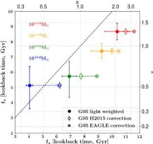
We use the same progenitor selection and mass functions of the previous chapter to measure the main progenitor stellar mass growth of galaxies as a function of stellar mass atz∼0.1, and measured the assembly time, which we defined as the time at which half the total mass of the descendent was assembled. We compare this assembly time to the light-weighted stellar ages from a sample of low-redshift SDSS galaxies from the literature. Our findings suggest that massive galaxies form a higher proportion of their mass ex-situ than lower-mass galaxies. We compare our timescales to the EAGLE simulation, as well as the semi-analytic models of Henriques et al. (2015). We find the semi-analytic models perform better than EAGLE in reproducing the observed stellar mass versus assembly time and light-weighted stellar ages. This work appeared in Hill et al. (2017b).

Chapter 4

In this chapter, we investigate the median flattening through the axis ratio of galax-ies atz<0.5 in the CANDELs fields, and its relationship to parameters such as stellar mass, sersic index, and size. We find that at atz<2, quiescent galaxies are rounder than their star-forming counterparts, however atz>2the median appar-ent axis ratios are indistinguishable, suggesting the structure in star-forming and quiescent galaxies at high redshift are similar. We also find that in star-forming galaxies, atz<1, the median axis ratio depends strongly on stellar mass, whereas quiescent galaxies do not show the same dependence. The strongest observable dependence for quiescent galaxies is sersic index. For star-forming galaxies, the size is the best predictor for flattening, with larger star-forming galaxies exhibiting smaller axis ratios. From our findings, we believe that the axis ratio is tracing the bulge-to-total galaxy mass ratio which would explain why smaller/more massive star-forming galaxies are rounder than their extended/less massive analogues, as well as why we do not observe strong mass and size dependencies in quiescent galaxies, as the majority of the quiescent population is not expected to have a strong disk complement. This work is to be submitted.

Chapter 5

(19)

sur-vey, with a measured photometric redshift ofz=2.4 (Muzzin et al. 2012). From the discrepancy in the spectroscopic and photometric redshifts, we highlight the importance of spectroscopy for redshift determination for red objects with prom-inent rest-frame optical breaks. From the spectrum, we measure a stellar velocity dispersion and are able to determine a dynamical mass which is a more direct method and avoids the pitfalls of estimating mass than through the SED, with the associated uncertainties in the initial mass function and effects of dust. We are also able to confirm quiescence through strong Balmer absorption and the absence of any emission lines, as well as establish that intermediate mass galaxies do quench at these redshifts. This work appeared in Hill et al. (2016).

References

Behroozi, P. S., Marchesini, D., Wechsler, R. H., et al. 2013, ApJL, 777, L10 Bezanson, R., van Dokkum, P., & Franx, M. 2012, ApJ, 760, 62

Bezanson, R., van Dokkum, P. G., Tal, T., et al. 2009, ApJ, 697, 1290

Brammer, G. B., Whitaker, K. E., van Dokkum, P. G., et al. 2011, ApJ, 739, 24 Clauwens, B., Franx, M., & Schaye, J. 2016, MNRAS, 463, L1

Henriques, B. M. B., White, S. D. M., Thomas, P. A., et al. 2015, MNRAS, 451, 2663

Hill, A. R., Muzzin, A., Franx, M., & Marchesini, D. 2017b, ApJL, 849, L26 Hill, A. R., Muzzin, A., Franx, M., et al. 2017a, ApJ, 837, 147

Hill, A. R., Muzzin, A., Franx, M., & van de Sande, J. 2016, ApJ, 819, 74 Hilz, M., Naab, T., & Ostriker, J. P. 2013, MNRAS, 429, 2924

Hopkins, P. F., Bundy, K., Hernquist, L., Wuyts, S., & Cox, T. J. 2010, MNRAS, 401, 1099

Hopkins, P. F., Cox, T. J., Younger, J. D., & Hernquist, L. 2009, ApJ, 691, 1168 Hubble, E. P. 1925, Popular Astronomy, 33

Hubble, E. P. 1929, Proceedings of the National Academy of Science, 15, 168 Ilbert, O., McCracken, H. J., Le F`evre, O., et al. 2013, A&A, 556, A55 Madau, P., & Dickinson, M. 2014, ARA&A, 52, 415

Marchesini, D., Muzzin, A., Stefanon, M., et al. 2014, ApJ, 794, 65

McLure, R. J., Pearce, H. J., Dunlop, J. S., et al. 2013, MNRAS, 428, 1088 Morishita, T., Ichikawa, T., Noguchi, M., et al. 2015, ApJ, 805, 34

Moustakas, J., Coil, A. L., Aird, J., et al. 2013, ApJ, 767, 50 Muzzin, A., Labb´e, I., Franx, M., et al. 2012, ApJ, 761, 142

Muzzin, A., Marchesini, D., Stefanon, M., et al. 2013a, ApJS, 206, 8 —. 2013b, ApJ, 777, 18

Newman, A. B., Ellis, R. S., Bundy, K., & Treu, T. 2012, ApJ, 746, 162

Ownsworth, J. R., Conselice, C. J., Mortlock, A., et al. 2014, MNRAS, 445, 2198 Papovich, C., Finkelstein, S. L., Ferguson, H. C., Lotz, J. M., & Giavalisco, M. 2011, MNRAS, 412, 1123

(20)

REFERENCES

Schreiber, C., Pannella, M., Elbaz, D., et al. 2015, A&A, 575, A74 Torrey, P., Wellons, S., Machado, F., et al. 2015, MNRAS, 454, 2770 Trujillo, I., Ferreras, I., & de La Rosa, I. G. 2011, MNRAS, 415, 3903

van Dokkum, P. G., Whitaker, K. E., Brammer, G., et al. 2010, ApJ, 709, 1018 van Dokkum, P. G., Leja, J., Nelson, E. J., et al. 2013, ApJL, 771, L35

van Dokkum, P. G., Bezanson, R., van der Wel, A., et al. 2014, ApJ, 791, 45 Williams, C. C., Giavalisco, M., Cassata, P., et al. 2014, ApJ, 780, 1

(21)

(22)

Chapter

2

The Mass, Color, and

Structural Evolution of

Today’s Massive Galaxies Since

z

∼

5

In this paper, we use stacking analysis to trace the mass-growth, colour evolution, and structural evolution of present-day massive galaxies (log(M∗/M)=11.5) out to z = 5. We utilize the exceptional depth and area of the latest UltraVISTA data release, combined with the depth and unparalleled seeing of CANDELS to gather a large, mass-selected sample of galaxies in the NIR (rest-frame optical to UV). Progenitors of present-day massive galaxies are identified via an evolving cumulative number density selection, which accounts for the effects of merging to correct for the systematic biases introduced using a fixed cumulative number density selection, and find progenitors grow in stellar mass by ≈ 1.5 dex since

z = 5. Using stacking, we analyze the structural parameters of the progenitors and find that most of the stellar mass content in the central regions was in place byz∼2, and while galaxies continue to assemble mass at all radii, the outskirts experience the largest fractional increase in stellar mass. However, we find evidence of significant stellar mass build up atr <3 kpc beyond z >4 probing an era of significant mass assembly in the interiors of present day massive galaxies. We also compare mass assembly from progenitors in this study to the EAGLE simulation and find qualitatively similar assembly withzatr<3 kpc. We identifyz∼1.5as a distinct epoch in the evolution of massive galaxies where progenitors transitioned from growing in mass and size primarily through in-situ star formation in disks to a period of efficient growth inre consistent with the minor merger scenario.

Allison R. Hill, Adam Muzzin, Marijn Franx, et al. The Astrophysical Journal

(23)

2.1 Introduction

The mass growth and structural evolution of today’s most massive galaxies is an important tracer of galaxy assembly at early times. These systems are host to the oldest stars, suggesting they were the first galaxies to assemble. Because they are the oldest systems, their progenitors can theoretically be traced to higher redshifts than their low mass counterparts and can be studied from the onset of re-ionization to give a complete history of galactic evolution. Additionally, the most massive systems tend to be the most luminous, and they are the easiest to observe at high redshift with high fidelity. Massive galaxies also provide important constraints on the physics involved in cosmological simulations, as they impose upper limits on growth as well as the efficiency of various feedback mechanisms such as active galactic nuclei, mergers and supernovae.

Today’s massive (log M∗/M ∼ 11.5) galaxies, to first order, are a uniform population. They are homogeneous in morphology and star formation, appearing spheroidal and have low specific star formation rates, and high quiescent fractions (e.g., Thomas et al. 2005; Gallazzi et al. 2005; Kuntschner et al. 2010; Thomas et al. 2010; Cappellari et al. 2011; Mortlock et al. 2013; Moustakas et al. 2013; Ilbert et al. 2013; Muzzin et al. 2013b; Davis et al. 2014; McDermid et al. 2015). In contrast to today’s massive galaxies, massive galaxies at high redshift show increasing diversity (e.g., Franx et al. 2008; van Dokkum et al. 2011). With increasing redshift, massive galaxies become increasingly star forming (e.g., Papovich et al. 2006; Kriek et al. 2008; van Dokkum et al. 2010; Brammer et al. 2011; Bruce et al. 2012; Ilbert et al. 2013; Muzzin et al. 2013b; Patel et al. 2013a; Stefanon et al. 2013; Barro et al. 2014; Duncan et al. 2014; Marchesini et al. 2014; Toft et al. 2014; van Dokkum et al. 2015; Barro et al. 2016; Man et al. 2016; Tomczak et al. 2016), and the massive galaxies which are identified as quiescent at high redshift are structurally distinct from their low redshift counterparts as seen in their small effective radii (re) and more centrally concentrated stellar-mass density profiles (Daddi et al. 2005; Trujillo et al. 2006; Toft et al. 2007; Cimatti et al. 2008; van Dokkum et al. 2008; Damjanov et al. 2009; Newman et al. 2010; Szomoru et al. 2010; Williams et al. 2010; van de Sande et al. 2011; Bruce et al. 2012; Muzzin et al. 2012; Oser et al. 2012; Szomoru et al. 2012, 2013; McLure et al. 2013; van de Sande et al. 2013; Newman et al. 2015; Straatman et al. 2015; Hill et al. 2016).

(24)

Sample Selection

the epoch when galaxies’ central regions assemble their mass.

Obtaining a census of massive galaxies across a broad redshift range is tech-nically challenging, as they have low number densities on the sky (Cole et al. 2001; Bell et al. 2003; Conselice et al. 2005; Marchesini et al. 2009; Bezanson et al. 2011; Caputi et al. 2011; Baldry et al. 2012; Ilbert et al. 2013; Muzzin et al. 2013b; Duncan et al. 2014; Tomczak et al. 2014; Caputi et al. 2015; Stefanon et al. 2015; Huertas-Company et al. 2016) and their rest-frame optical emission shifts into the near-infrared (NIR) at intermediate redshifts. To study the evolution of massive galaxies across cosmic time, as a population, necessitates deep and wide NIR surveys to both probe large volumes and obtain rest-frame optical emission to significant signal-to-noise (S/N).

In this study we use stacking analysis to obtain high-fidelity profiles of the progenitors of massive galaxies out to significant radii (at lowz, r>60 kpc). We take advantage of the unparalleled combination of depth and area in the third data release of the UltraVISTA survey (McCracken et al. 2012) to study the structural evolution of massive galaxies out toz=3.5. Due to incompleteness in UltraVISTA at the highest redshifts considered in this study, we also use the deeper CANDELS F160W data from the 3DHST photometric catalogs (Brammer et al. 2012; Skelton et al. 2014; Momcheva et al. 2016) to extend the redshift coverage toz=5. This is a significant gain in redshift over previous studies, and provides the most extensive redshift range over which the profiles of massive galaxies have been traced.

2.2 Sample Selection

2.2.1 Number-density selection

Linking the progenitors of present day galaxies to their high redshift counterparts is challenging, as the merger and star formation history (SFH) of any individual galaxy is not well constrained. One way to circumvent these issues is to assume that galaxies maintain rank-order across cosmic time (i.e., the most massive galaxies today will have been the most massive galaxies yesterday, cosmologically speak-ing). This assumption predicts a constant co-moving number-density with redshift, an outcome used by van Dokkum et al. (2010) to trace the mass and size growth of galaxies from z= 2 (corresponding to n =2×10−4 _Mpc−3_dex−1_{). Subsequent}

studies have used the same assumptions to select progenitors based on a constant cumulative number density (e.g., Bezanson et al. 2011; Brammer et al. 2011; Pa-povich et al. 2011; Fumagalli et al. 2012; van Dokkum et al. 2013; Patel et al. 2013a; Ownsworth et al. 2014; Morishita et al. 2015), which has the advantage over its non-cumulative counterpart of being single valued in mass.

(25)

cos-mology to connect progenitors and their descendants. It is important to note, that we have used the prescription to traceprogenitorsof low redshift massive galaxies, not thedescendantsof high redshift massive galaxies, of which the former yields a steeper evolution in cumulative number density due to the shape of the halo mass function, and scatter in mass accretion histories (see Behroozi et al. 2013; Leja et al. 2013).

2.2.2 The implied stellar mass growth of the progenitors of

massive galaxies since

z

∼

5

In Fig. 3.1 we show the integrated Schecter fits of the mass functions of Muzzin et al. (2013b) between0.2<z<3.0, and Grazian et al. (2015) between3.5<z<5.5. These mass functions are based on photometric redshifts determined via ground and space based NIR imaging from the UltraVISTA and CANDELS surveys re-spectively. In the left-panel of Fig. 3.1, we show our evolving cumulative number density selection based on the abundance matching of Behroozi et al. (2013). The masses implied from a fixed-cumulative number density selection are also shown to illustrate the effect of the bias when the effects of mergers are ignored in the selection. In the right-panel of Fig. 3.1 the implied progenitor masses from the left-panel are plotted for both the fixed and evolving cumulative number density selection, as a function of redshift. The error bars are the uncertainties from the mass functions, which take into account the uncertainties in the photometric red-shifts, SFHs, and cosmic variance. The solid grey region represents the scatter in the number densities from the abundance matching of Behroozi et al. (2013), and the hatched regions illustrate an estimate of the mass completeness which is discussed in detail in Sec. 2.2.3.

Belowz=2, Fig. 3.1 shows that both constant and evolving cumulative num-ber density selections yield progenitor masses which are consistent within the un-certainties in the mass-functions. However beyond z = 2, the bias in the fixed cumulative number density becomes significant, and over-predicts the median pro-genitor mass. Using the abundance matching technique, we see an overall increase in stellar mass of 1.5 dex sincez∼5. Our fractional mass growth out to z=3 is consistent within the uncertainties with Marchesini et al. (2014) who use the same abundance matching selection for ultra-massive log(M∗/M)∼11.8) descendants, and with Ownsworth et al. (2014), who use a constant cumulative number density selection which is corrected for major mergers to trace progenitors. Using their correction, they find75±9%of the descendant mass is assembled afterz=3, which is consistent with∼80%which we find in the current study.

(26)

(27)

linearly interpolated the mass between adjacent redshift bins. We also observe a trend of the uncertainties in the mass function monotonically increasing from low to high redshift. Thus, we similarly linearly interpolated the uncertainties to estimate the uncertainty in mass for3.0<z<3.5due to uncertainties in photo-z, SFH and cosmic variance. We also use the uncertainties in the progenitor mass selection as the upper and lower mass bounds for the galaxies that contribute to the resulting stack, thus we select a larger range of masses at higher redshift, than at lower redshift.

It has been shown that the Behroozi et al. (2013) prescription for selecting progenitors performs well in terms of recovering the average stellar mass of the progenitors of present-day high-mass galaxies, however this method fails in captur-ing the diversity in mass of all progenitors as implied by simulations (e.g., Torrey et al. 2015; Clauwens et al. 2016; Wellons & Torrey 2016), which also predict that the scatter in progenitor masses tends to increase with redshift. Given this large scatter, there is no guarantee that the evolution of other galaxy properties, such as size, will follow from the Behroozi et al. (2013) selection. However, in an upcoming paper (Clauwens et al., in prep) we will show that for the property of interest in our study (i.e. the average radial build-up of stellar mass for the progenitors of massive galaxies), the Behroozi et al. (2013) selection yields average agreement with progenitors within the EAGLE simulation.

2.2.3 Data

UltraVISTA

In order to study the evolution of the average properties of massive galaxies, it was necessary to utilize both wide field ground-based, and deep space-based imaging for our stacking analysis. Massive galaxies (log(M∗/M)∼11) are exceedingly rare objects, with low number densities (∼ 10−5 Mpc−3) on the sky (e.g., Cole et al. 2001; Bell et al. 2003; Baldry et al. 2012; Muzzin et al. 2013b; Ilbert et al. 2013; Tomczak et al. 2014; Caputi et al. 2015; Stefanon et al. 2015), and require wide-field surveys to characterize a significant population. To that end, we utilize the NIR imaging from the DR3 of the UltraVISTA survey (McCracken et al. 2012) for our stacking analysis.

The DR3 UltraVISTA catalog (Muzzin et al., in prep) is a K-selected, multi-band catalog constructed from the UltraVISTA survey. Briefly, the survey covers the COSMOS field with a total area of1.7 deg2_{, with deep imaging in the}_Y_,_J_,_H_and

K sbands. The survey also contains ultra-deep stripes with longer exposures which cover a0.75 deg2 _{area, and also includes imaging in the VISTA NB118 NIR filter}

(Milvang-Jensen et al. 2013). The newest data release is constructed with the same techniques as the DR1 30-band catalog (Muzzin et al. 2013a), with the inclusion of new and higher-quality data to determine photo-z’s, and stellar population parameters. The DR3 survey depths in the ultra-deep stripes are∼1.4magnitudes deeper than DR1 (with5σlimiting magnitudes in the ultra-deep regions of 25.7, 25.4, 25.1, and 24.9 inY,J,H andK s).

(28)

Sample Selection

NB816). Most importantly for this analysis we also include the latest data from SPLASH (Capak et al. 2012) and SMUVS (PI Caputi; Ashby et al., in prep). These are post-cryo Spitzer-IRAC observations that improve the [3.6] and [4.5] depth from 23.9 to 25.3. Overall this is a 38-band catalog (compared to 30 in Muzzin et al. 2013a), and the substantial increase in depth in theY,J,H,K s,[3.6] and[4.5]bands make it a powerful dataset for studying massive galaxies at inter-mediate and high redshifts.

In the right panel of Fig. 3.1 we have indicated our estimated mass completeness limits with the filled hatched regions. To estimate our mass completeness atz<4, we used the limits on the mass functions from Muzzin et al. (2013b) (which were derived using UltraVISTA DR1), and adjusted the mass limit according to the gain in K-band depth (the K-band limit is 1.5 magnitudes deeper between DR1 and DR3) assuming a constant mass-to-light ratio. Since galaxy mass-to-light ratios decrease with redshift (e.g. van de Sande et al. 2015), this likely represents a conservative estimate of the limiting mass at high redshifts.

CANDELS

As UltraVISTA DR3 is only mass complete for our selection out toz = 3.5, we use the reddest band available from CANDELS in order to explore redshifts un-obtainable through UltraVISTA. We select galaxies using the photometric data products from the 3DHST survey (Brammer et al. 2012; Skelton et al. 2014) from all 5 CANDELS fields. As an estimate of our mass completeness in CANDELS, we adopt the limiting mass derived from the75% magnitude completeness limit (F160W = 25.9) in the shallower pointings in the GOODS-S and UDS fields as described in Grazian et al. (2015). They estimated their mass completeness using the technique of Fontana et al. (2004), which assumes the distribution of mass-to-light ratios immediately above the magnitude limit holds at smass-to-lightly lower fluxes, and compute the fraction of objects lost due to large mass-to-light ratios. The estimated completeness for CANDELS is indicated in the right panel of Fig. 3.1 as the grey cross-hatched region.

Although the aforementioned estimates of mass completeness take into account galaxies with varied mass-to-light ratios, it is worth stressing inherent uncertainties when determining mass limits at high redshift. Atz>3.5, we increasingly rely on photometric redshifts, as high-fidelity spectroscopic redshifts are fewer in number (Grazian et al. 2015). In addition, sub-mm galaxies (SMGs) likely account for at least a fraction of the progenitors of massive galaxies at high redshift (e.g., Toft et al. 2014), and they have been shown to have high optical extinction (e.g., Swinbank et al. 2010; Couto et al. 2016). As the progenitors selected atz>3.5of this study tend to be less massive than a typical SMG, we do not expect that they will form a significant fraction of the sample. However, we cannot rule out a tail of less, but still obscured sources to lower masses in the distribution of SMGs. This would have the effect of biasing our high redshift progenitor selection to bluer, less-obscured sources.

(29)

Table 2.1. Number of galaxies in each redshift range by catalog

z-range UV IS T A 3DHS T

0.2<z<0.5 16 0

0.5<z<1.0 56 5

1.0<z<1.5 96 22

1.5<z<2.0 166 31

2.0<z<2.5 276 79

2.5<z<3.0 466 104

3.0<z<3.5 160 69

3.5<z<4.5 ... 110

4.5<z<5.5 ... 154∗ ∗_{We are incomplete in mass for this} point

Note. — Above are the number of galaxies found within the mass ranges outlined in Fig. 3.1.

density selection (see Sec. 2.2.1) from both the UltraVISTA and 3DHST catalogs. In order to boost the number of galaxies in UltraVISTA, we have used galaxies from both the deep (DR1) and ultra-deep (DR3) catalog out to2.0<z<2.5where we are complete in mass for the shallower catalog (DR1). For the3.0<z<3.5bin, we have only utilized the DR3 catalog, as we are incomplete in DR1. As evident from Table 4.1, UltraVISTA has a larger population of massive galaxies at low redshift, while there are 0 galaxies in all 5 CANDELS fields which are massive (log(M∗/M)∼11.5) atz=0.35, and only 5 galaxies in the next highest redshift bin. However CANDELS is crucial to continue the progenitor selection beyond

z>3.5 as we are mass incomplete in this region with UltraVISTA. Additionally, as galaxies had smallerreat high redshift (see discussion in Sec. 5.1 and references therein), the space-based seeing of CANDELS is necessary to properly map the density profiles at these epochs. Thus we utilize both data sets in our analysis.

2.3 Rest-Frame Color Evolution

Cumulative number density selection is a method which selects solely on stellar mass, and is therefore blind to other galaxy properties such as levels of star-formation activity. A simple, but effective way to establish star-forming activity in a population of galaxies is to observe where they are located in rest-frameU−V

andV−Jcolor space, commonly referred to as aUV J-diagram. First proposed by Labb´e et al. (2005), it is observed that galaxies exhibit a bi-modality in rest-frame

UV J colour space which is correlated with the level of obscured and unobscured star formation. Actively star-forming and quiescent galaxies separate into a ‘blue’ and ‘red’ sequence in theUV J-diagram (e.g., Williams et al. 2009, 2010; Whitaker et al. 2011; Fumagalli et al. 2014; Yano et al. 2016).

(30)

Rest-Frame Color Evolution

(31)

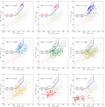
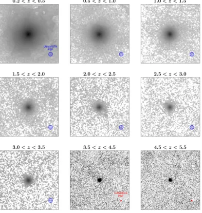
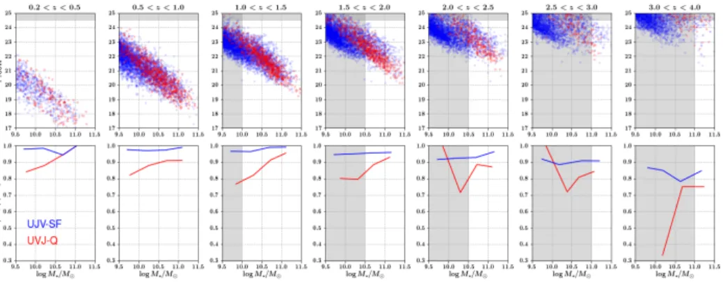
provide a diagnostic of star-formation activity within each stack. Each of the nine panels represents a different redshift range, with galaxy masses selected according to their expected evolving cumulative number density (see Fig. 3.1). The first seven panels are galaxies from UltraVISTA DR3, and the last two panels contain galaxies from the 3DHST photometric catalog. It is important to note that we are mass incomplete for the4.5<z<5.5bin (see Fig. 3.1). However we have chosen to include it as part of our analysis, with the caveat that we are likely biased towards bluer galaxies. Overlaid in each panel are the colour selections used by Muzzin et al. (2013b) to separate quiescent and star forming sequences.

As one progresses in redshift, it becomes apparent from Fig. 5.2 that the num-ber of galaxies selected dramatically increases. This is a result of two competing effects. The first, is that the size of our mass range becomes progressively larger with redshift, as seen in the error bars on the right-panel of Fig. 3.1. By selecting in a wider mass range, we will inevitably select more galaxies. The second effect is that as the number densities of progenitors increases with redshift, we are progress-ing towards the lower mass end of the mass-functions (Ilbert et al. 2013; Muzzin et al. 2013b; Grazian et al. 2015). Thirdly, at low redshift, the probed co-moving volume is also smaller than at high redshift. The combined effect is to have our lowest redshift, and least populated stack contain only 16 galaxies, whereas our most populated stack at2.5<z<3.0 contains 276 objects (Table 4.1).

The most prominent trend in Fig. 5.2 comes in the colour evolution of the progenitors across redshift. They begin very blue in both U −V and V −J in the lower-left of the forming sequence and progress red-ward along the star-forming sequence to the upper-right until2.5 <z<3.0 before reddening inV−J

and joining the quiescent sequence. Assuming our number density selection is valid, this represents a true evolution inUV J colour.

Fig. 2.3 show the averageUV Jcolour evolution for each redshift bin, separated into star-forming and quiescent progenitors, and highlights explicitly the trends observed in Fig. 5.2. In this figure, we see most of the early (z>3) colour evolution is driven by the star-forming progenitors. Atz<3, star-forming progenitors are beginning to quench in large numbers and the two tracks are broadly parallel until

z<1 where the quiescent progenitor fractions are high, andUV J colour evolution is driven by the quiescent progenitors. This seems to indicate that massive galax-ies begin their existence as star forming galaxgalax-ies, which progress along the blue sequence (via aging of the stellar populations, and increase in stellar mass through star formation), before quenching and joining the red sequence.

(32)

Evolution in Far-Infrared Star Formation Rates

Figure 2.3 Above is the average rest-frameUV Jcolour evolution for the progenitors of the quiescent (red symbols) and star-forming (blue symbols) progenitors. The entire sample is plotted in small grey symbols to best illustrate the scatter. The size of the red and blue symbols indicates the quiescent/star-forming fraction (e.g., a large red circle correspond to a high quiescent fraction, and a small blue circle corresponds to a low star-forming fraction). The redshift evolution proceeds from bottom-left to top-right. Purple arrows indicate the direction of quiescence and are labelled for points which bracket a quiescent fraction of20%. Thez=5point is plotted as an open circle to remind the reader that we are incomplete in that redshift bin, and are likely biased to bluer galaxies.

galaxy properties between the samples is likely attributed to differences in stellar mass.

(33)

Figure 2.4 TheFIR implied star formation rates (dashed blue line), compared to the derivative of the mass-redshift evolution (solid black line), with their associated uncertainties (shaded regions). The implied mass assembly from star formation is higher than the derivative of the mass evolution, atz>1.5, and lower at z<1.5. At low redshifts, we see the star formation rates drop precipitously, and that mass assembly cannot be proceeding via in-situ star formation, and growth is likely merger driven.

2.4 Evolution in Far-Infrared Star Formation Rates

In Fig. 5.2 and Fig. 2.3, we see evidence that the evolution of massive galaxies can be broadly separated into two epochs. Atz>1.5, galaxies have colours which are consistent with growth mainly through in-situ star formation. At z < 1.5, galaxy colours are consistent with quenched systems, with mergers becoming the dominant mechanism for growth. We can estimate this epoch more directly by comparing star formation rates to the mass assembly implied from the evolving cumulative number density selection.

(34)

Analysis

via the relation from Kennicutt (1998), with a factor of 1.6 correction to convert between the Salpeter IMF used in Kennicutt (1998), to the Chabrier IMF used for the DR3 catalog.

In order to more directly compare the net stellar mass growth as implied from the abundance matching technique to the stellar mass growth from star formation, a 50%conversion factor has been applied to the SFR to account for stellar mass which is lost in outflows from stellar winds (see van Dokkum et al. 2008, 2010). From Fig. 2.4, we see that SF is able to account for all of the stellar mass growth at

z>1.5, with little to no contribution from mergers. In contrast, the SFR atz<1.5 are insufficient to explain the mass growth, suggesting stellar mass is accreted via mergers.

Between 1.5 < z < 2.5, the stellar mass growth predicted from star forma-tion is greater than what is found from the abundance matching techniques by 0.1−0.2 dex. This discrepancy is also seen in model and observation comparis-ons (see Somerville & Dav´e 2015; Madau & Dickinson 2014), with potential for the FIR SFRs to be over estimated during this epoch (see Madau & Dickinson 2014 and discussion therein). In spite of this, the FIR SFR support the notion that massive galaxies grow via star-formation untilz∼1.5, where merger driven growth dominates, consistent with the rest-frameUV J colours, and what is found in the literature (see Sec. 5.1 and references therein).

2.5 Analysis

2.5.1 Stacked Images

For galaxies atz<3.5, images were stacked using4800×4800cutouts taken from the UltraVISTA mosaics, which contain both deep and ultra-deep stripes. For each cut-out, SEDs were generated using the ancillary data available in the UltraVISTA and CANDELS source catalogs. These SEDs were used to flag potential active galactic nuclei (AGN), which were removed from the resultant stack. The indi-vidual cut-outs were also visually inspected to remove objects which were identified as doubles, or triples (i.e., were not separated by SExtractor; Bertin & Arnouts 1996) or in close proximity to saturated stars to maintain image fidelity. In total,

<4%of the entire sample was discarded.

Cutouts were centered using coordinates taken from the UltraVISTA DR1 (only deep stripes) and DR3 (only ultra-deep stripes) catalogs, with cubic spline interpol-ation performed for sub-pixel shifting. For galaxies atz>3.5, images were stacked using2400×2400 cutouts, taken from the 5 CANDELS fields (AEGIS, COSMOS, GOODS-S, GOODS-N and the UDS), with images centred using the coordinates from the 3DHST photometric catalogs (Brammer et al. 2012; Skelton et al. 2014) with sub-pixel shifting also performed using cubic spline interpolation.

(35)

(36)

Analysis

For the UltraVISTA stacks, the ultra-deep and deep cutouts were weighted differently in the final stack as the ultra-deep stripes have an exposure time a factor ∼ 10× greater than the deep stripes. The images are weighted by the expected S/N gain, based on the exposure time (i.e. an image with a factor of

∼10more exposure time, will result in a S/N gain of∼3). The exact exposures varied between the Y, J, H and Ks bands, with the relative weights between the deep and ultra-deep also changing slightly.

The cutouts were normalized to the sum of the flux contained in the central 1.500×1.500 (corresponding to10×10 pixelfor UltraVISTA images and25×25 pixel for CANDELS images). A weighted sum was performed on the masked cutouts, with the cutouts contained in the ultra-deep stripes given a heavier weight than those in the deep stripes. This summed image was divided by the weight-map to provide the final stack.

For the UltraVISTA stacks, PSFs were generated similarly to the stacked-galaxy images. Stars within a magnitude range were chosen such that the stars had sufficiently high S/N without being saturated (≈16.5 K s-band magnitude). The stars were treated in the same manner as the stacks of the galaxies (i.e. normalized and averaged). To account for variations in the PSF across the mosaic, 12 different PSFs for each band were generated corresponding to 12 different regions of the mosaic ultra-deep stripes, and 9 for the deep stripes. A final PSF for the relevant band was generated from a weighted average of the 12/9 PSFs, with the weights corresponding to the number of galaxies from each field that went into the making of the stack. Thus, each stack has a uniquely generated PSF.

For the CANDELS F160W stacks, PSFs for each of the 5 fields were taken from the 3DHST-CANDELS data release (Grogin et al. 2011; Koekemoer et al. 2011; Skelton et al. 2014). In a similar manner to the UltraVISTA stacks, the PSF for the relevant band was generated from a weighted average of the PSF from each field, with the weights corresponding to the number of galaxies from each field that contributed to the final stack, thus each F160W stack similarly has a uniquely generated PSF.

Fig. 2.5 displays the results from the stacking analysis. Each panel contains a 24×2400_{display of one of the UltraVISTA bands (either Y,J,H, or Ks), except the} last two panels which are stacks of the CANDELS F160W data. The UltraVISTA stacks are all displayed at the same colour scale to highlight the differences in background, which increases with increasingz. The F160W stacks were plotted at a different colour scale for clarity, as the background is much higher.

In addition to the stacks in Fig. 2.5, 100 bootstrapped images were also gen-erated for each stack to constrain uncertainties in the structural parameters de-termination (see Sec. 2.5.2). Each bootstrapped image also comes with its own unique PSF that reflects the proportion of galaxies from various fields in the same manner as the original stacked images.

2.5.2 Sersic Profile Fitting

(37)

Figure 2.6Top: Best-fit effective radius in units of arc seconds as a function ofzfor all bands. Points originating from UltraVISTA are plotted in black, with different symbols corresponding to the specific bands as indicated in the legend. HST

(38)

Analysis

being to restrict the value of the Sersic indices to between 1 < n < 6. Fig. 2.6 shows the best fitre and n for each band, and each redshift bin, with the uncer-tainty derived from the1σdistribution of the bootstrapped fits. The UltraVISTA derived values are in black, with each symbol corresponding to a different band. The F160W values are indicated with red diamonds, with the last symbol plotted unfilled to mark where we are incomplete. The HWHM of the UltraVISTA and CANDELS PSFs are indicated on the top panel in light-grey and dark-grey re-gions respectively. As seen from the top panel of Fig. 2.6, we resolve the stacked images to within an effective radius for UltraVISTA belowz=2, and thereis fully resolved for CANDELS in all redshift bins. Additionally, for the redshift bins for which we have stacks for CANDELS and UltraVISTA, the derived sizes and Ser-sic indices are roughly consistent with one another, suggesting our ground-based structural parameters are reliable.

Absent from Fig. 2.6 are best-fit values forreandnbelowz=1for the F160W band. In these redshift bins, at the mass ranges considered, there were no galaxies present in the catalogue to contribute to a stack (see Table 4.1). Similarly, best-fit values for the UltraVISTA bands are not present for all redshift bins with the Y, J, H and Ks dropping out at z=2,2.5,3 and 3.5 respectively, due to insufficient signal-to-noise in the resultant stack (and that we are incomplete in UltraVISTA atz>3.5).

2.5.3 Evolution in

r

e

Due to the progression of redshift between the stacks, there and nare measured at varying rest-frame wavelengths. In order to measure as closely as possible the same rest-frame wavelength, we have measured how re and n change with wavelength. In the left panel of Fig. 2.7 we have plotted re as a function of rest-frame wavelength. Different colours correspond to different redshift bins, and different symbols demarcate the observed band (with the same symbol convention as in Fig. 2.6). The desired rest-frame wavelength of0.5µm was chosen to minimize extrapolation, as well as still be red-ward of the optical-break.

Atz<3, we have measurements in multiple bands, and find the effective radii decrease with increasing rest-frame wavelength which is consistent with results from previous studies (e.g., Cassata et al. 2011; Kelvin et al. 2012; van der Wel et al. 2014; Lange et al. 2015). However between 2 < z < 3, the uncertainties are consistent with little to no evolution inrewith rest-frame wavelength. When

(39)

(40)

Analysis

representative of there at0.5 µm. This is assuming that the size-gradient will be flat for low-mass, late-type galaxies at high redshift.

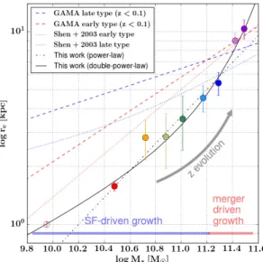
Figure 2.8 The implied mass-size evolution of the progenitors of massive galaxies. Circles are measurements from the stacks from the present study, with each point representing a different redshift. There plotted above are the same values taken from the right-panel of Fig. 2.7. Symbol color plotting convention is the same as Fig. 3.1, with the lowest-zpoints corresponding to the most massive galaxies, and monotonically decreasing to the highest-z. We have plotted the highest-zpoint as an open face symbol to remind the reader we are mass incomplete for thatz-bin. Plotted above are theg-band local mass-size relations for late (dashed blue line) and early type (dashed red line) galaxies from the GAMA survey (Lange et al. 2015), as well as the mass-size relations from Shen et al. (2003). For the lowest 2z

bins (i.e. z<1), our galaxies fall precisely on the local mass-size relation for early type galaxies, but are systematically below the relations at higherz. Also plotted above are the best fit single and double power-law relations to our data.

In the right panel of Fig. 2.7, we have plotted re at 0.5 µm as a function of

(41)

not surprising, and the consistency is reflected in the right panel of Fig. 3.1, where atz<2, the mass of the progenitors chosen using a fixed vs. evolving cumulative number density are within the uncertainties in both the mass function and the semi-analytic models. Although we measure a slightly steeper relation than van Dokkum et al. (2010), it is surprising how well the relation is extrapolated at

z > 2 given that we are selecting galaxies which are distinct in mass from the fixed-cumulative number density selection.

In Fig. 2.8 we investigate the evolution of the mass-size plane. We have taken the values of re from the right panel of Fig. 2.7, and plotted them against their respective progenitor masses, with the highest mass associated with the lowest redshift bin. For comparison purposes, we have over-plotted the mass-size relations from Shen et al. (2003) and Lange et al. (2015) for both early and late type galaxies. For Lange et al. (2015), who investigate the mass-size relations as a function of rest-frame wavelength, we use their g-band relations which corresponds most closely to a rest-frame wavelength of0.5µm. The measuredrefrom our stacking analysis fall on the SDSS and GAMA mass-size relations for early-type galaxies atz<0.1. However for all other redshift bins, our galaxies fall below the local-mass size relation, consistent with van Dokkum et al. (2010). Also plotted in Fig. 2.8 are simple single (dash-dot line) and double (solid line) power-law fits of the form

re=aM_∗b (2.1)

re=γM_∗α 1+M∗

M0

!α−β

(2.2)

From Fig. 2.8, we see that the double power-law is a more appropriate fit for our data, with the parameters γ = 2.9×10−4_, _α ₌ ₀_._35, _β ₌ ₂_.₁_×₁₀3 _and

log(M0/M)=14.77. Continuing with the plotting convention in previous figures, our 4.5 < z < 5.5 point has been plotted as an open-face symbol to highlight incompleteness issues within that bin. It is interesting to note that this point has not been included in any of the power-law fits, and the fact that it falls on on the extrapolation of the double power-law is not designed.

(42)

Analysis

2.5.4 Evolution in

n

Fig. 2.10 is analogous to Fig. 2.7, except we investigate how the Sersic index n

changes with rest-frame wavelength in place ofre. From the left panel of Fig. 2.10 we see little to no evolution innwith wavelength at any redshift. We have therefore taken an average n weighted by the bootstrapped uncertainty in each band to measure a representativenfor each redshift bin. Atz>3where we only have one measurement for each stack, the measurement was considered representative. The resulting values are plotted in the right panel of Fig. 2.10.

Fig. 2.10 shows a clear downward trend of n with redshift, consistent with previous findings outz=2(e.g., van Dokkum et al. 2010). This trend is also ex-pected given the evolution in the quiescent fraction. Actively star forming galaxies tend to have lowern/are more centrally concentrated than their quiescent coun-terparts (e.g., Lee et al. 2013; Freeman 1970; Lange et al. 2015; Mortlock et al. 2015), thus at z >1 the decrease in n is likely driven by morphological changes between each redshift bin which we also see reflected in the evolution of the mass-size relations (Fig. 2.8). van Dokkum et al. (2010) also foundn to decrease with redshift, although their relation is steeper than the one measured in the current study. However the n−z relation from van Dokkum et al. (2010) was derived from galaxies atz< 2, where the slopes are comparable, but where we measure systematically highern.

2.5.5 Mass Assembly

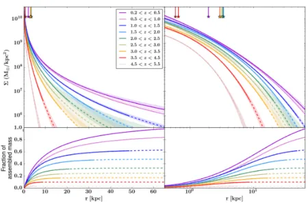
Equipped with measurements ofre andn, we can investigate surface-density pro-files, and mass assembly as a function of radius. To generate these propro-files, we have assumed that the mass-to-light ratio is constant across the profile, and that all the mass can be found within a radius of75 kpc. Given these assumptions, and that the integrated mass within 75 kpc must equal the total mass found in the right panel of Fig 3.1 (i.e., the same constraints used in van Dokkum et al. 2010), we have generated stellar-mass density profiles which can be found in Fig. 2.9.

Fig. 2.9 shows the Sersic fits using the values of re andn for each redshift bin in the right panels of Fig. 2.7 and Fig. 2.10 respectively. The transition between the solid and dashed lines for each profile marks the point when the error in the background becomes significant. Since many of the values ofre and n are either interpolated, or averaged (see Sec. 2.5.3 and Sec. 2.5.4), the profiles from which this transition point was determined were the closest to the rest-frame wavelength of0.5µm (these are the same bands which are displayed in Fig. 2.5).

(43)

Figure 2.9Top: The projected surface mass-density profiles for our stacks (presen-ted in both log-linear and log-log scales). Each profile is a Sersic, with thereand

(44)

(45)

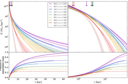
In Fig. 2.11, we have divided the surface mass density profile for each redshift bin from Fig. 2.9 by the surface mass density profile at0.2<z<0.5. In this way, we are able to trace the fractional mass assembly as a function of radius. At the highest redshift bins, we see the central regions are the first to form, with very little of the stellar mass beyond3 kpcin place atz∼5. Between3.0<z<4.5, we see rapid growth, with the fraction of mass assembled in the inner regions more than doubling. It is also in this redshift interval that a not insignificant fraction of stellar mass is assembled between3 and 10 kpc. We can trace the redshift of formation as a function of radius by tracing the horizontal dashed-line in Fig. 2.11, which marks the point at which half of the stellar mass was assembled. As you trace from small to large radii, the dashed line crosses different coloured regions, indicating that the interior regions were the first to assemble, with the outer regions assembling at later and later times, indicative of ‘inside-out’ growth.

Figure 2.11 The fractional build-up of stellar mass, as a function of radius, as-sembled at various z intervals (i.e. each mass profile in Fig. 2.9 divided by the mass profile for 0.2 < z<0.5). The horizontal dashed lines markes the 50% as-sembly point, and the vertical dot-dashed line is drawn at the 3 kpc point for clarity. From this plot, the formation redshift for the interior vs. exterior re-gions can be seen, with the inner rere-gions containing 50% of their final stellar mass between2.0<z<3.0, with the outer regionzof formation lagging behind.

We can trace this growth quantitatively by considering the total mass in and outside the3 kpc boundary. We have de-projected the surface density profiles of Fig. 2.9, and separated the mass growth into stellar mass assembly that is within

(46)

Analysis

and is the same mass assembly seen in the right panel of Fig. 3.1. From the red line, we see continuous, albeit decelerating, mass assembly from z =5 to z =0. This is inconsistent with previous works such as van Dokkum et al. (2010) and Patel et al. (2013a) who found the interior regions are consistent with no assembly sincez=2, oft cited to be evidence of ‘inside-out’ growth, although it depends on precisely what is meant by this term.

Figure 2.12 The total projected mass within3 kpc(red-line) and outside3 kpcas implied by integrating the profiles from Fig. 2.9. The last symbol is plotted as open faced to remind the reader that we are mass incomplete in thatz-bin. There is growth in both radial regions, however the growth is not self-similar with the growth outsider=3 kpcproceeding at a faster pace than the inner regions.

It is important to note from Fig. 2.11 and Fig. 2.12 that even though the regions outside3 kpcexperience a greater growth rate than the inner regions, there is still significant mass build-up fromz=5to z=0 in the interior. Although the growth between the inner and outer regions is not self-similar, the growth is not necessarily ‘inside-out’ as described in previous works (e.g., van Dokkum et al. 2010; van de Sande et al. 2013), especially when considering the mass assembly atz >3. At these redshifts, significant stellar mass is assembled at all radii (although mass accretion is concentrated in the central regions).

2.5.6 Comparisons with simulations

(47)

Vogelsberger et al. 2014; Schaye et al. 2015). In fact, the EAGLE simulation has been calibrated to reproduce the galaxy stellar mass function atz=0. However, there remain few examples (e.g, Snyder et al. 2015; Wellons et al. 2015) in the literature which explicitly compare the evolution of structure in simulations to observations . In this section, we endeavour to make such a comparison.

Figure 2.13 Above show the the build-up of stellar mass inside (red line) and out-side (blue line) a3 kpcaperture as predicted by the EAGLE simulation, as well as the total stellar mass evolution (black line). The faded colours is the mass evolution from this study, with the colours corresponding to the same regions as the simulations. The simulations show rapid build up of the outer regions, which is qualitatively similar to the data. The main difference between the observa-tions and the simulaobserva-tions is the total mass evolution proceeds more rapidly in the simulations, with most of the effects see in the build up of the outer regions.

(48)

Discussions and Conclusions

amounted to 24 galaxies. The aperture masses from EAGLE quoted above are averages from the progenitors of these 24 galaxies.

A qualitative comparison between the simulations and the observations show remarkable agreement. For the mass within3 kpc, the agreement is always within a factor of 2, which is within the uncertainty associated with the assumptions made when determining stellar masses from photometry (Conroy et al. 2009). Both methods predict the same overall trend i.e. that there is a steady build up of stellar mass within3 kpc, and rapid assembly at later times at radii larger than3 kpc. The main difference between the simulations and observations is that EAGLE predicts a more rapid assembly of the progenitors. The progenitors in EAGLE must assemble more mass in the same period of time in order to result in the final stellar mass oflog M∗/M=11.5at z∼0.3. This offset is not entirely unexpected, given differences between the evolution of the observed and simulated galaxy stellar mass functions at high-zin the mass ranges considered for this study (∼1010−1011 M, Furlong et al. 2015).

The progenitors in EAGLE must assemble more mass in the same period of time in order to come to the same descendant mass by z ∼ 0.3; and given the agreement with observations at r < 3 kpc, nearly all of this mass growth must occur in the outer regions. This suggests the progenitors in EAGLE are more centrally concentrated than observed, except at z > 4. Between 4 < z < 5, the fraction of stellar mass outside a 3 kpc aperture is broad agreement with the observations, which does not follow the trend atz < 4. One possible reason for this is the effective radius at these redshifts is close to1 kpc, which suggests nearly all of the total bound mass in the galaxy would be within3 kpc, which is not true at lower redshifts.

Some caveats that could affect the above comparison are some assumptions that were made in the observations, in particular the assumption of a constant mass-to-light ratio for our surface mass density profiles. If there is a strong gradient of stellar age with radius in the progenitors, and the interiors are older (which would be consistent with what we see in Fig. 2.11), then we would over-predict the fraction of the total stellar mass which is located at large radii, bringing us closer to agreement with the simulations. A similar effect would be expected if there are also strong gradients in dust. An analysis of forthcoming virtual observations from EAGLE with the effects of dust and inter-cluster light taken into account would be a better comparison, the investigation of which is beyond the scope of this paper.

Some assembly required: the structural evolution and mass assembly of galaxies at z<5

The following handle holds various files of this Leiden University dissertation:

http://hdl.handle.net/1887/61630

Author: Hill, A.

Title: Some assembly required: the structural evolution and mass assembly of galaxies at

z<5

Some Assembly Required:

The Structural Evolution and Mass Assembly

of Galaxies at

z

<

5

Proefschrift

Table of Contents

Chapter

1

Introduction

1.1

The Birth of Extra-Galactic Astronomy

1.2

Tracing Galaxy Evolution Using Integrated

Properties

1.3

Progenitor Selection

1.4

The Structural Evolution of Galaxy

Progen-itors

1.5

Galaxy Ages and Assembly Times

1.6

This Thesis

References

Chapter

2

The Mass, Color, and

Structural Evolution of

Today’s Massive Galaxies Since

z

∼

5

2.1

Introduction

2.2

Sample Selection

2.2.1

Number-density selection

2.2.2

The implied stellar mass growth of the progenitors of

massive galaxies since

z

∼

5

2.2.3

Data

2.3

Rest-Frame Color Evolution

2.4

Evolution in Far-Infrared Star Formation Rates

2.5

Analysis

2.5.1

Stacked Images

2.5.2

Sersic Profile Fitting

2.5.3

Evolution in

r

2.5.4

Evolution in

n

2.5.5

Mass Assembly

2.5.6

Comparisons with simulations

2.6

Discussions and Conclusions

2.6.1

Mass and size growth at

z

<