ESSAYS IN FINANCIAL ECONOMICS
Sunjin Park
A dissertation submitted to the faculty at the University of North Carolina at Chapel Hill in partial fulfillment of the requirements for the degree of Doctor of Philosophy in the Department
of Finance in the Kenan-Flagler Business School.
Chapel Hill 2017
Approved by: Riccardo Colacito Mariano M. Croce Eric Ghysels Anh Le
c
2017
Sunjin Park
ABSTRACT
Sunjin Park: Essays in Financial Economics (Under the direction of Riccardo Colacito)
ACKNOWLEDGMENTS
I would like to emphasize that my Ph.D. career at the Kenan-Flagler Business School would not have been possible without the support and encouragement of many wonderful people I met and have known.
I am indebted to my advisor Riccardo Colacito for his invaluable mentorship and dedication in directing my doctoral education. I am grateful to Eric Ghysels for his continued support and guidance since my Masters program and to Christian Lundblad for his valuable feedback and on-going encouragement on various aspects. I am also indebted to Anh Le for his endless support and patience from the very beginning of my research career. Lastly, I thank Mariano Croce for serving as a committee member and providing insightful feedback.
I have benefited tremendously from the conversations with my Ph.D. colleagues as well as the faculty members in our department. I am appreciative of their comments on my research as well as suggestions as a researcher and a presenter, all of which I do not take for granted.
I am grateful to my parents, my brother and my friends for their encouragement and caring throughout my academic training in Chapel Hill over the past 12 years. Finally, I would like to emphasize my gratitude to my wife Youngeun for her endless love and for bringing to the world our soon-to-be-born baby girl.
TABLE OF CONTENTS
LIST OF TABLES vi
LIST OF FIGURES vii
1 GLOBAL MACROECONOMIC CONDITIONAL SKEWNESS
AND THE CARRY RISK PREMIUM 1
Introduction . . . 1
1.1 Literature Review . . . 3
1.2 Model . . . 6
1.2.1 Setup of the Economy . . . 6
1.2.2 Equilibrium and Solution of the Model . . . 8
1.2.3 Asset Pricing . . . 10
1.2.4 Skewness in Forecasts and Carry Risk Premium . . . 11
1.2.5 Dynamic model . . . 16
1.3 Global Measures of Risk: Data Sources and Stylized Facts . . . 19
1.4 Empirical Results . . . 23
1.4.1 Predictive Regressions of Currency Returns . . . 24
1.4.2 Robustness . . . 33
1.4.3 Trading Conditional on Global Skewness . . . 34
1.5 Conclusion . . . 36
2 RISK AND RETURN TRADE-OFF IN THE U.S. TREASURY MARKET 37 Introduction . . . 37
2.1 Motivating Exercises . . . 41
2.2 Model . . . 45
2.2.1 The Risk-Neutral Dynamics and Bond Pricing . . . 46
2.2.3 Econometric Identification . . . 50
2.2.4 Discussion of Modeling Choices . . . 52
2.3 Results . . . 53
2.3.1 Estimation . . . 54
2.3.2 Model Diagnosis . . . 55
2.3.3 Parameter Estimates . . . 57
2.3.4 Economic Significance . . . 60
2.3.5 Matching Return Predictability and Conditional Volatilities in the Data . . . 63
2.4 Conclusion . . . 63
A APPENDIX 66 A.1 Appendix for: Global Macroeconomic Conditional Skewness and the Carry Risk Premium . . . 66
A.2 Appendix for: Risk and Return Trade-off in the U.S. Treasury Market . . . 74
LIST OF TABLES
1.1 Regression from simulated data . . . 19
1.2 Start date of forecasts data and summary statistics of the number of forecasters . . . 21
1.3 Predictive regression results of carry returns onto global measures . . . 25
1.4 Predictive regressions of individual buckets of currencies onto global skewness . . . . 30
1.5 Predictive regressions of individual buckets of currencies onto global expected growth . . . 31
1.6 Regressions of carry trade returns onto global skewness and other explanatory variables . . . 34
1.7 Summary statistics of the ordinary carry returns and the new strategy returns . . . 36
2.1 Predictability of weekly excess returns . . . 43
2.2 Validating model choices . . . 56
2.3 Parameter estimates . . . 58
2.4 Two robustness checks of the model . . . 59
2.5 Risk premium decomposition . . . 61
A.1 Calibration of the two-period model . . . 66
A.2 Calibration of the dynamic model . . . 67
A.3 Details about foreign exchange rate data . . . 68
A.4 Predictive regression results with the exclusion of the recent crisis . . . 69
A.5 Predictive regression results with global measure aggregated by taking the first principal component . . . 70
A.6 Predictive regression results with global measure aggregated by taking the GDP-weighted average . . . 71
A.7 Predictive regression results with alternative global measures . . . 72
LIST OF FIGURES
1.1 Subjective probability density function for each agent . . . 7
1.2 Global skewness, carry risk premia and interest rates . . . 11
1.3 Individual agent’s consumption over the possible endowment shocks . . . 12
1.4 Global measures of risks . . . 22
1.5 Estimated beta loadings for different sets of currencies . . . 27
1.6 Comparison of cumulative returns to the ordinary carry and the new strategy . . . . 35
2.1 Model-implied risk premium . . . 62
2.2 Campbell-Shiller regression coefficients . . . 64
CHAPTER 1 GLOBAL MACROECONOMIC CONDITIONAL SKEWNESS AND THE CARRY RISK PREMIUM
Introduction
The carry trade is a well known investment strategy that exploits the profitability of borrow-ing in the low interest rate currencies to invest in the high interest rate currencies. In this pa-per I document that the time-variation in the distribution of global growth prospects has pre-dictive power for carry trade returns. I study the macroeconomic risks that the carry trade in-vestor faces. Interestingly, I find evidence that the time-variation in conditional skewness in global growth prospects has significant predictive power, namely that a one standard deviation decline in the skewness measure increases the next-quarter carry trade risk premium by 5.24% per annum. The novel contribution of the paper is that global macroeconomic conditional skew-ness plays an important role in the variation in the carry risk premium.
I empirically test if the variation in the cross-sectional measures of macroeconomic prospects explains the currency market. I collect analysts’ forecasts for the growth rates of real GDP for a list of major countries including nine of the G10 countries as well as China. The currencies of these countries constitute 85.75% of the total foreign exchange turnover1. The individual fore-casts are contributed by analysts in different sectors of the economy and are collected primar-ily by Consensus Economics and Bloomberg. At each point in time and for each country, I con-struct measures of the cross-sectional mean, dispersion and skewness of the distribution of fore-casts across analysts. Then for each quarter, I calculate the cross-sectional average of the means across countries and, similarly, the average of the dispersion and the average of the skewness across countries. This yields time-varying measures of the distribution of, what I shall refer to as,
global growth prospects. The main empirical strategy proposed in this paper tests if my proposed global measures predict carry trade returns in the time-series.
1
I find evidence that the time-variation in global conditional expected growth and global con-ditional skewness can help predict next-quarter carry trade returns. The estimated coefficients are negative, indicating that when global expected growth or global skewness is low or negative, subsequent carry trade returns tend to be high or positive, i.e., yielding a positive risk premium. Notably, global skewness appears to be the most robust predictor among the different moments, especially as I repeat the exercise with strategies based on a larger set of currencies of up to 33 developed and emerging markets. I conduct a series of robustness tests, such as forming dynamic and static portfolios, changing the number of currencies in the formation of portfolios, and aggre-gating country-specific measures, e.g., by taking the first principal component or by computing the GDP-weighted average across countries. I also try jointly regressing on the global skewness measure along with other known explanatory variables.
A key benefit of my approach is that it yields a time-varying proxy for conditional skewness of macroeconomic growth prospects. A skewness measure is related to, but has an interesting dis-tinction from, the notion of disaster. Disasters are one-sided by nature and are often referred to as events that rarely happen. On the contrary, I observe frequent fluctuations of my skewness measure between positive and negative domains, even outside of times of heightened concerns about severe recessions. Moreover, my empirical strategy allows obtaining real-time measures based on a collection of professional forecasters’ views each time a survey is reported, thus reveal-ing information about macroeconomic prospects that are otherwise not easy to detect. Further-more, my results are robust to the exclusion of the Great Recession of 2008-09, confirming that they are not driven by extreme left-tail events.
I build a model in which agents have heterogeneous beliefs, so that it can be mapped directly to my empirical investigation. In this economy, there are two countries, each populated by three agents. In each country, one agent has the correct beliefs about the future growth rate of the economy, while the other two agents have expectations that are either larger (”the optimist”) or smaller (”the pessimist”) than the true growth rate. Depending on the specific degree of op-timism and pessimism of those two agents, the cross-sectional distribution of beliefs within each country can take on any possible extent of skewness.
Assuming that financial markets are complete, the exchange rate between the currencies of the two countries is equal to the ratio of marginal utilities of the two agents with correct beliefs by a simple no-arbitrage argument (as in Backus, Foresi, and Telmer (2001)).
Let us consider the situation in which the cross-sectional skewness is negative in one country and equal to zero in the other country. According to the definition that I adopt in my empir-ical approach, this situation corresponds to one in which the global skewness is negative. It is intuitive to conclude that the risk-free rate should be lower in the first country, in which the pes-simist drives up the demand for the risk-free asset by a larger extent. Carry trade would thus involve borrowing in the currency of the first country with negative skewness and investing in the currency of the other country with zero skewness.
A key feature of the model with heterogeneous beliefs is that agents want to consume the most in states of the world that they think are the most likely. This means that the marginal investor consumes less than the pessimist in bad times. This helps explain why shorting the cur-rency of the negatively skewed country is a risky strategy. In bad times, the marginal utility (consumption) of the marginal investor goes up (drops) more in the negatively skewed country. This, by no-arbitrage, results in an appreciation of the currency of this country. Equivalently, the carry trade is risky because it loses money in bad times. A similar argument can be used to show that it gains money in good times.
This example illustrates why the risk premium is higher in times in which the global skewness is more negative. Based on this idea, the model implies that carry trades are risky when the in-vestor faces negatively skewed global prospects.
1.1 Literature Review
Siwasarit (2016) find that negative cross-sectional skewness precedes recessions and helps pre-dict future stock returns. I base upon some papers that study the source of the cross-sectional dispersion of GDP forecasts (Patton and Timmermann (2010) and Andrade, Crump, Eusepi, and Moench (2016)) and interpret the cross-section of forecasts as macroeconomic disagreement among forecasters.
I argue in this paper that my measure of macroeconomic conditional skewness is a global mea-sure of risk. The implication for the currency market is that the global meamea-sure should affect the stochastic discount factors of countries based on the exposure to the risk so that the movement of the foreign exchange rate is also affected. This fits in with the literature following Lustig, Rous-sanov, and Verdelhan (2011) that currency risk premia can be explained by the exposure to a systematic risk. I focus on the risks about macroeconomic growth based on the evidence that the currency risk premia can be explained by consumption growth risk as documented in Lustig and Verdelhan (2007). Specifically given my model with disagreement, currency risk premia are driven by the cross-sectional skewness in growth forecasts because the resultant risk-sharing among agents will drive the stochastic discount factors and hence also drive the riskiness in the foreign exchange rate.
The literature has been studying the dispersion of analysts’ forecasts and its asset pricing implications. Anderson, Ghysels, and Juergens (2005) find that dispersion in analysts’ forecasts about expected earnings is a priced factor in the equities market. Buraschi, Trojani, and Vedolin (2014) provide evidence that belief disagreement, also constructed from earnings forecasts, can explain the cross-section of corporate bond and stock returns.
model of Dumas, Lewis, and Osambela (2016) home and foreign investors disagree because of their differing interpretations of home versus foreign news, and one implication of the model is the co-movement of returns and international capital flows.
We may relate the role of skewness to that of disaster risk. Farhi and Gabaix (2016) and Farhi, Fraiberger, Gabaix, Ranciere, and Verdelhan (2015) find that rare disaster risk can ac-count for a large fraction of the carry trade risk premia. However, notice that a measure of skew-ness is not restricted to the notion of a rare, extreme event. In fact, my time-series of global macroeconomic conditional skewness tends to be low, well in advance of the onset of the reces-sions. Moreover, a skewed distribution in growth prospects has the further benefit that it mea-sures both negative and positive directions of asymmetry, which cannot be captured by disaster risk.
The literature provides many competing explanations for currency risk premia, one of which emphasizes the role of commodities. In the model of Ready, Roussanov, and Ward (2014), the high interest rate countries, which correspond to the investment currencies, tend to be the com-modity exporters, while the low interest rate countries, which correspond to the funding curren-cies, tend to be the exporters of the finished goods. The authors show empirical support that the strategy of sorting based on net exports in basic goods, which measure how much one special-izes in producing and exporting basic commodities, yields high returns. Chen, Rogoff, and Rossi (2010) and Bakshi and Panayotov (2013) provide empirical evidence on the relationship between exchange rates and commodity prices.
dom-inating other macro uncertainty variables like the dispersion in GDP forecasts. My paper looks specifically at the GDP forecasts and instead examines different moments of the distribution.
My paper also sheds some perspectives on the macro-finance literature that bridges inter-national asset prices and consumption dynamics. Colacito and Croce (2013) provide evidence that the highly correlated long-run growth prospects can explain the Backus and Smith (1993) anomaly that the correlation between consumption differentials and exchange rate movements is low. Gourio, Siemer, and Verdelhan (2013) develop a standard real business cycle framework, in which the risk premia vary with the probability of a disaster that leads to a decline in invest-ment. My measures of global risks are not directly from consumption or growth data, but they are derived from analysts’ views of future real economic growth prospects.
This paper is organized as follows. Section 2 introduces a model that yields testable predic-tions. Section 3 provides an explanation on the forecasts data and highlights stylized facts about the proposed global measures of risks. Section 4 presents the main currency predictability results. Lastly, section 5 provides concluding remarks.
1.2 Model
In the following section I focus on a static model with heterogeneous agents to highlight the economic mechanism of how the cross-sectional skewness in forecasts affects the riskiness of a currency trade. The static model can be understood as a snapshot of the dynamic version which follows subsequently.
1.2.1 Setup of the Economy
Consider a two-period, complete market economy with two countries, which I call home and foreign. The home country produces good X, and the foreign country produces good Y. The true data generating processes for the endowment goods X and Y are as follows
logX= logX0+εX logY = logY0+εY (1.1)
where the endowment shocksεX ∼ N(µ, σ2) and εY ∼ N(µ, σ2) have a correlation ofρ.
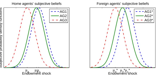
Home agents’ subjective beliefs
Subjective probability density functions
µ3 µ2µ1
Endowment shock
Foreign agents’ subjective beliefs
µ3* µ
2*µ1*
Endowment shock AG1
AG2 AG3
AG1* AG2* AG3*
Figure 1.1: Subjective probability density function (pdf) for each agent. Each line corresponds to each agent’s subjective pdf about the endowment shock of his respective country. µi orµ∗i
corresponds to the subjective mean forecast made by an agent. Above is an illustration on a 2-dimensional graph, but in my model endowment shocks (εX, εY) have an additional dimension.
the foreign country. Each agent forms a subjective probability density function about the en-dowment shocks. I assume that all agents correctly form the underlying distributional shape, the variance and the covariance of the shocks but that agents can have biased expectations about the mean of the shocks, which I will interchangeably refer to as the forecast or the prediction. For each country, there will be an optimist and a pessimist as well as an unbiased forecaster whose prediction coincides with the correct mean. Furthermore, for simplicity I assume that all agents correctly forecast the mean of the other country’s endowment shock. Mathematically, each home agentAGi forms a joint probability distribution πi(εX, εY) ∼ N((µi, µ)0,Σ), and each foreign
agentAG∗i formsπi∗(εX, εY) ∼ N((µ,µ∗i)0,Σ). In the coming discussion I will denote each agent
by sorting agents within a country based on the means on a descending order: AG1 forms the highest mean, whileAG3 forms the lowest mean.
Figure 1.1 presents an example in which the three home agents form much more negatively skewed set of forecasts about their endowment shocks relative to the foreign agents. I define
effect of variance, or dispersion, across forecasts. Notice that, because the cross-sectional variance across agents’ predictions are all fixed to be the same, negatively skewed set of forecasts must accompany a pessimist being extremely pessimistic as well as an optimist whose prediction is rel-atively close to that of the unbiased agent. Details of the calibration can be found in Table A.1.
I discipline the skewness of forecasts in each country α andα∗ to be entirely determined by the global skewness αg. Specifically,
α=δαg α∗ =δ∗αg
In the language of the dynamic model, the time-series variation in the skewness in each country will be only driven by the global skewness and not by idiosyncratic shocks. Although this is a simplification, I impose it in the interest of obtaining a global measure of risk and abstracting away from idiosyncratic risks.
In terms of the preferences of the economy, I assume that agents have power reward functions with risk aversion parameterγ and subjective discount factor β. I also assume for simplicity that agents have complete home bias in the consumption of goods. This means the home agents will only consume goodX, and the foreign agents will only consume good Y. Finally, I assume that all six agents currently constitute the same, one-sixth share of the overall economy.
1.2.2 Equilibrium and Solution of the Model
The social planner optimizes the weighted average of the expected utility of each agent with Pareto weights λi and λ∗i. Since the model has only two periods, the planner forms the optimal
allocation by choosing next period consumption for each agentCi andCi∗
Π =λ1E1 h
βC 1−γ
1
1−γ
i
+λ2E2 h
βC 1−γ
2
1−γ
i
+λ3E3 h
βC 1−γ
3
1−γ
i
(1.2) +λ∗1E1∗
h
βC
∗1−γ
1
1−γ
i
+λ∗2E2∗
h
βC
∗1−γ
2
1−γ
i
+λ∗3E3∗
h
βC
∗1−γ
3
1−γ
i
(1.3)
with each expectationEi orEi∗ taken over the subjective distributionπi orπ∗i formed by the
of the economy, the Pareto weights attached to agents are all equal by assumption. This can be interpreted as a particular snapshot of the dynamic model in Section 1.2.5 at a point in which the Pareto weights happen to be all equal like in the steady state.
As a result of complete home bias, the social planner satisfies the following budget constraints
X=X1+X2+X3 and Y =Y1+Y2+Y3 (1.4)
whereXi is the home agent AGi’s optimal consumption of the home goods X next period, and Yi is the foreign agent AG∗i’s consumption of the foreign goodsY next period. I will use Xi,0 and
Yi,0 to denote the current period consumption, which is equal across all agents based on our as-sumption that all agents currently are of equal size.
Upon solving the above optimization problem we can write down the allocation next period as
Ci =
π1i/γ
P3
i=1π 1/γ i
×X (1.5)
Ci∗ = (π
∗
i)1/γ
P3
i=1(πi∗)1/γ
×Y (1.6)
1.2.3 Asset Pricing
The home (or foreign) interest rate can be computed via the marginal utility of any home (foreign) agent. To see this, the subjective marginal utility of a home agent can be written as
˜
Mi=β
Ci Ci,0
−γ (1.7) =β 1 3 γ
exp{−γεX}
π11/γ+π21/γ+π31/γ
γ 1
πi
(1.8)
which is useful for pricing the bond in the home country
B =Ei[ ˜Mi] =E
˜
Mi πi
π
| {z }
M
(1.9)
where the expectation Eis taken over the true underlying objective distributionπ. The second
equality helps write the price of a bond in terms of the true, objective marginal utilityM by ap-pending an adjustment term πi/π to the subjective marginal utility. Hence, upon adjusting for
an agent’s misperception, asset pricing can be done by any agent in the economy. The price of the bond can be written as
B=E
β 1 3 γ
exp{−γεX}
3 X
i=1 (πi)1/γ
γ 1
π
(1.10)
I denote the interest rate on the risk-free bond asi=−log(B) and similarly for the foreign coun-try i∗.
With the assumption that financial markets are complete, the change in the real exchange rate between the two countries is
∆s= logM∗−logM (1.11)
−0.5 0 0.5 0
0.2 0.4 0.6 0.8 1
Carry risk premium (%)
Global skewness
−0.5 0 0.5 7.7
7.8 7.9 8 8.1 8.2 8.3
Interest rates (%)
Global skewness Home
Foreign
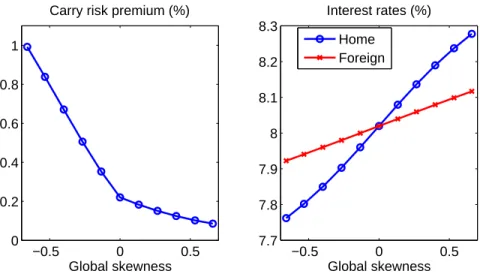
Figure 1.2: Global skewness, carry risk premia and interest rates. Comparative statics of chang-ing global skewness αg, which drives home forecasts to be more skewed than foreign (δ > δ∗). The left and right panels show the resulting carry risk premium and the interest rates for each country, respectively.
1.2.4 Skewness in Forecasts and Carry Risk Premium
From a currency investor’s perspective, the excess return on investing in the foreign currency and shorting the home currency can be written ascxr = i∗ −i+ ∆s. Since the carry trade is taking a long position in the currency of the higher interest rate country while shorting the other currency, the carry risk premium in levels can be written as
carry risk premium =
logE[exp{i∗−i+ ∆s}] ifi∗> i
logE[exp{−(i∗−i)−∆s}] ifi∗< i
Let us consider the comparative statics of varying global skewness αg, which will drive each
coun-try’s skewness in forecast. I specify δ > δ∗, so that the home country’s forecast skewness α is driven by global skewnessαg to a larger extent than the foreign country. This is to generate
dif-ference in riskiness between the two countries. In our exercise, any change in global skewnessαg
will drive the home forecasts to be more skewed than the foreign forecasts whether it be negative or positive.
−0.05 0 0.05 0.1 −0.15
−0.1 −0.05 0 0.05 0.1 0.15
Endowment shock
Log consumption growth
Home agents
−0.05 0 0.05 0.1 −0.15
−0.1 −0.05 0 0.05 0.1 0.15 0.2
Endowment shock Foreign agents
AG1 AG2 AG3
AG1* AG2* AG3*
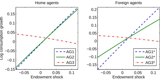
Figure 1.3: Individual agent’s consumption over the possible endowment shocks. For illustration on a 2-dimensional graph, I display only the diagonal slice of the (εX, εY) domain in which εX
and εY are equal in value. Above is the case ofα =−0.9 and α∗ =−0.3.
premium rises. The time-series implication that is testable in the data is that if more negative global skewness tends to be followed by higher average excess returns on the carry.
The right panel indicates that the skewness in forecasts has implications for the sorting of in-terest rates. Notice that on the negative domain of skewness, the home inin-terest rate is lower than the foreign rate. Recall that on the negative domain, the home skewness α is more negative than foreign skewness α∗. In this region, the pessimist of the home country is so pessimistic that he will drive up the overall demand for the risk-free bond for precautionary motives and thus push down the equilibrium interest rate at home. The opposite happens in the positive domain in which α > α∗ because the optimist drives down the overall demand for bonds. Thus, the home interest rate is higher than the foreign interest rate on the positive domain.
From the investor’s point of view, the sorting of interest rates is important. When the skew-ness in forecasts is negative, the carry trade would involve investing in the foreign currency and shorting the home currency, while the long-short position would be swapped when the skewness in forecasts is positive instead. In addition to determining the investment strategy for the carry, the home and foreign interest rates also affect the level of the carry risk premium. The risk pre-mium will be determined by the sign and magnitude of the foreign exchange rate component rel-ative to the interest rate differential.
skewed than the foreign forecasts. Figure 1.3 plots individual log consumption growth rates over the possible realizations of the endowment shocks. Notice that the optimal consumption of the unbiased agent in the foreign country (AG∗2) is roughly in the middle of that of the optimist and the pessimist. On the contrary, the unbiased agent of the home country (AG2) consumes more ”like” the optimistAG1. This is because the subjective belief of the unbiased agent AG2 is close to that of the optimist AG1 yet very far from that of the pessimist AG3 as observed in Figure 1.1.
The economic interpretation of the consumption path of AG2 is that in the bad state of the worldAG2 ends up providing large insurance to the pessimist of the home country, resulting in a low consumption for himself. Recall the determinants of each agent’s optimal consumption shown in Equation (1.5). Because of the subjective probability density in the numerator, each agent will want to consume more in the states that he thinks are the most likely. Since the bad state of the world is the state in which the pessimist is more correct, the pessimist enjoys a larger share of the pie, leaving less for AG2 to consume.
What does the consumption ofAG∗2 and AG2 imply for asset pricing? Recall that these agents are those with the unbiased predictions about the underlying distribution of endowment shocks. This makes their consumption directly applicable for computing the (objective) marginal utility of consumption in each country
M =β
C2
C2,0 −γ
and M∗=β
C2∗ C2∗,0
−γ
(1.12)
so I will often refer to these agents as the marginal agents within the respective countries. The above marginal utility of consumption will drive the growth rate in the foreign currency value as previously mentioned
∆s= log(M∗)−log(M) (1.13)
more relative to the foreign agent’s. That makes the foreign exchange rate to depreciate, which would be a loss to the carry investor because his investment currency, the foreign currency, is val-ued less in terms of the home currency. Upon a good endowment shock in both countries, the home marginal agent now consumes relatively more than the foreign marginal agent, instead. This is because the home marginal agent’s consumption contract is relatively similar to that of the home optimist, both of which serves as the party highly disagreeing with the home pessimist. Since the home marginal agent happened to be quite correct in making prediction, he enjoys a large consumption along with the optimist in the same country. Consequently, ∆swould appre-ciate, delivering a positive return to the carry investor. Importantly, notice that the above carry trade is risky strategy to implement because the investor loses in the bad state of the world. The no-arbitrage argument suggests that prices would adjust so that there should be a high risk pre-mium for implementing this risky strategy.
In order to fully characterize the riskiness of the strategy in this two-country environment, I will also need to consider what happens in the case of a bad endowment shock in one country and a good shock in another country. Consider the case of a bad shock at home but a good shock abroad. The foreign marginal utility of consumption will be low, while the home marginal utility of consumption will be high, thus pushing down ∆swith the same sign. In addition, the home marginal agent suffers even more so because he had to provide significant insurance to the pes-simist based on the promised allocation. In other words, this combination of bad and good shock makes a bad news even worse. This causes ∆sto drop significantly, which contributes to an even higher risk for the carry strategy.
Now let us consider the case of global skewness αg being positive instead. Here the home skewness in forecasts α is larger than the foreignα∗, so keep in mind that the investment cur-rency is the home curcur-rency. The important distinction is that here AG2 serves more ”like” the pessimist AG3 in that he buys insurance from the optimist. That means the home marginal agent enjoys a large share of the pie upon a bad shock, which implies that a bad news is actually not too bad. As a result, the overall riskiness of the carry is not as high as the negative skewness case. Similarly by the argument of no-arbitrage, the less risky case of positive skewness would yield a lower carry risk premium compared to the negative skewness case.
domain is not as steep. This is due to the construction of the carry, in that the interest rate dif-ferential −(i∗−i)(>0) increases withαg, which pushes up the slope of the curve on the positive domain. Although the kink on the negative line could be of interest in future work, I argue that for now the negative association by itself is the primary object of interest. In my empirical exer-cise, I find no conclusive evidence regarding the magnitude or the specific location of a kink. As long as each country’s skewness is at least partially exposed to global skewness, the negative as-sociation between the skewness in forecasts and the carry risk premium should exist, and I only focus on this in this paper.
In summary, the negative association between the carry risk premium and the skewness in forecasts can be rationalized by the appropriate compensation for the consumption risk that is being faced by the marginal agent. When global skewness becomes more negative, in which case the home forecasts become more negatively skewed, the home marginal agent has to provide sig-nificant insurance to the pessimist in the bad state of the world thus causing the carry trade to become a risky strategy. In the empirical section, I test for the model implication in the time-series to see if the expected excess returns on the carry tend to be higher following a more nega-tive global skewness.
One comment to be made is that I assumed that the home forecast skewness is driven by global skewness to a larger extent than the foreign forecast skewness. I could alternatively con-sider the flip sideδ < δ∗. The interesting observation is that the carry risk premium again has the same pattern across global skewnessαg. The carry strategy will swap for the negative and positive skewness domains, but because of the switching of the strategy, the riskiness of the carry is identical. Hence, in terms of focusing on the carry risk premium, the more important assump-tion isδ 6= δ∗ regardless of the specific order. For the purpose of my study, I do not pin down which countries in the data correspond to the home or the foreign country in the model. As long as the exposure to global skewness is different across countries, the negative association between skewness in forecasts and the carry risk premium remains.
of research, my empirical work faces data limitation in that, for some countries in my sample, skewness is not tightly measured enough to tease out information about the idiosyncratic compo-nent. Hence, in my theory and empirical sections, I focus entirely on the systematic component based on the argument that for a large enough cross-section of currencies, only the systematic risk should be priced.
1.2.5 Dynamic model
The static model described above serves the purpose of highlighting the intuition of a model with heterogeneous beliefs. In this section, I discuss the dynamic model, which served as the ba-sis of the static version in terms of finding the optimal allocation. I develop an economy in which skewness in forecasts varies over time and thus drives the variation in the carry risk premium.
I similarly model an economy with two countries, each of which is occupied by three agents. Importantly, I allow time-variation in the beliefs of the optimists and the pessimists{µ1,t, µ3,t, µ∗1,t, µ∗3,t}, while the beliefs of the unbiased agentsµ2,t and µ∗2,t are kept equal to the true average
growth rate µ. Specifically I let the variation in the beliefs to be driven by the time-variation in skewness in forecasts
αt=
µ1,t+µ3,t−2µ2,t µ1,t−µ3,t
α∗t = µ
∗
1,t+µ∗3,t−2µ∗2,t
µ∗1,t−µ∗3,t (1.14)
In particular, I model the time-series such that the variable for global skewness follows an AR(1) process
agt =ρaagt−1+σaεa,t withεa,t∼ N(0,1) (1.15)
which drives each country’s skewness in forecasts determined by
at=δagt a
∗
t =δ∗a g
t (1.16)
For each individual country I employ the mappingαt = at/
p 1 +a2
t (and similarly forα∗t) to
resolve the issue that αt that is described in Equation (1.14) must be bounded between -1 and 1.
to the global skewness αgt compared to foreign skewnessα∗t. The calibration can be found in the Appendix in Table A.2. Although one can implement a more general time-series model of beliefs, I impose the above structure to keep it stylized so that I can highlight the role of time-varying skewness in forecasts.
I adopt a model with heterogeneous beliefs laid out in Anderson, Ghysels, and Juergens (2005). The social planner maximizes
Π = 3 X
i=1
λi,0 T X t=0 Ei,0 h βC 1−γ i,t
1−γ
i +
3 X
i=1
λ∗i,0
T X
t=0
Ei∗,0 h
βC
∗1−γ
i,t
1−γ
i
(1.17)
with initial Pareto weightsλi,0 and λ∗i,0. Again with perfect home bias and the budget constraint
Ci,t =Xi,t Ci,t∗ =Yi,t (1.18)
X1,t+X2,t+X3,t =Xt Y1,t+Y2,t+Y3,t=Yt (1.19)
for everyt, the planner chooses consumption{Ci,t, Ci,t∗ }to solve for the Pareto-optimal
alloca-tion.
The first order condition with respect to X1,t can be written as
λ1,0π1,t(ω|ω0)βtC1−,tγ−λ3,0π3,t(ω|ω0)βtC3−,tγ = 0 (1.20) λ1,0π1,t(ω|ω0)X1−,tγ =λ3,0π3,t(ω|ω0)
Xt−X1,t−X2,t
−γ
(1.21)
where the second line simplifies the first line and applies the budget constraint. ω denotes a state, i.e. a realization of the home and foreign endowment shocks. ωt denotes the history of the path of realizations up to timet. Let us recursively define Pareto weights as
λi,t(ω|ωt−1) =
λi,t−1(ωt−1)πi,t(ω|ωt−1)
P3
i=1λi,t−1(ωt−1)πi,t(ω|ωt−1) + P3
i=1λ∗i,t−1(ωt−1)πi,t∗ (ω|ωt−1)
(1.22)
λ∗i,t(ω|ωt−1) = λ
∗
i,t−1(ωt−1)πi,t∗ (ω|ωt−1)
P3
i=1λi,t−1(ωt−1)πi,t∗ (ω|ωt−1) +
P3
i=1λ∗i,t−1(ωt−1)πi,t∗ (ω|ωt−1)
(1.23)
condi-tion as
λ1,t(ω|ωt−1)X1−,tγ =λ3,t(ω|ωt−1)
Xt−X1,t−X2,t
−γ
(1.24)
A similar first order condition with respect toX2,t yields
λ2,t(ω|ωt−1)X2−,tγ =λ3,t(ω|ωt−1)
Xt−X1,t−X2,t
−γ
(1.25)
Combining these two, we can write the solution as
Ci,t =
λ1i,t/γ(ω|ωt−1)
λ11/γ,t (ω|ωt−1) +λ1/γ
2,t (ω|ωt−1) +λ
1/γ
3,t (ω|ωt−1)
×Xt (1.26)
Similarly repeat above for the foreign agents’ consumption to obtain
Ci,t∗ = λ
∗1/γ
i,t (ω|ωt−1) λ∗11,t/γ(ω|ωt−1) +λ∗1/γ
2,t (ω|ωt−1) +λ
∗1/γ
3,t (ω|ωt−1)
×Yt (1.27)
Notice that in the static model, which would be a snapshot of the dynamic setup, I do not have to keep track of the Pareto weights. Instead only the subjective beliefsπi matter as displayed in
Equation (1.5). Here, however, consumption also depends on the previous Pareto weightsλi,t−1.
One can think ofλi,t−1 as a term that accumulates the history of the realization of past con-sumption. The optimal consumption is then determined by agents’ subjective beliefs, adjusted for the current standing of the Pareto weights. Nonetheless, one can imagine the point in time such that all Pareto weights happen to be all equal. In that specific case, Equation (1.26) simpli-fies to a form like Equation (1.5). Consequently, the intuition of the result from the static model can be similarly applied to the dynamic model in that I expect the carry risk premium to be high when global skewness is more negative.
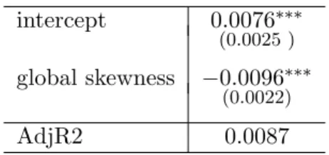
I perform a brief simulation exercise. Instead of simulating the model for a very long number of periods, I fix the number of periods toT = 20 and start over and repeat 100 times. The pur-pose of this is that I do not want to consider periods in which one of the agents ends up being infinitesimally small (λi,t≈0) which can happen after many periods.
intercept 0.0076∗∗∗ (0.0025 ) global skewness −0.0096∗∗∗
(0.0022)
AdjR2 0.0087
Table 1.1: Regression of the subsequent carry trade returns on global skewness αgt based on sim-ulation. The regressor is standardized. Statistical significance is calculated based on Newey-West standard errors.
level of global skewness αgt. Table 1.1 shows that the loading on global skewness is negative and statistically different from zero with sizable t-statistics. The magnitude of the loading is compa-rable to the magnitude of the unconditional risk premium, which is also positive and different from zero.
The above predictive regression suggests a negative time-series relationship between the carry risk premium and global skewness. The result is in line with the earlier discussion on the static model, and moreover it provides testable time-series implications.
1.3 Global Measures of Risk: Data Sources and Stylized Facts
Constructing a measure of conditional skewness on macroeconomic growth prospects is chal-lenging. The standard Pearson measure of skewness requires high frequency of data points for an appropriate time window given our interest in a conditional measure of skewness. For our purpose, measuring the time-varying skewness of macroeconomic variables then becomes far from obvious because most macroeconomic indicators are available only at quarterly frequency. Instead, I use the third moment from the cross-sectional distribution of individual forecaster’s macroeconomic forecasts. I construct global measures of risks by: (i) computing cross-sectional moments of each country and then (ii) aggregating across countries to obtain global expected growth, global uncertainty and global skewness. In terms of aggregation, I take the simple aver-age across countries, i.e. I take the averaver-age of each country’s expected growth across countries, and so forth. I also supply alternative specifications of aggregation as robustness tests, using the 1st principal component or taking the weighted average based on GDP weights.
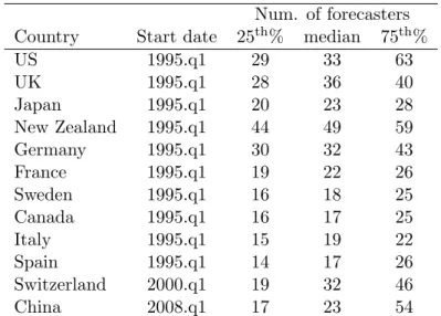
sur-veying reputable institutions of their forecasts of future macroeconomic variables for the major countries of the world. The publication provides individual forecasts of real GDP growth rates broken down by each forecaster. Bloomberg is another popular data source that makes available individual forecasts, but since only post-2008 data were available to me I augment Bloomberg data to the data from Consensus Forecasts. In addition, I also include a few country-specific forecasts datasets, one of which is New Zealand and is kindly provided by the Reserve Bank of New Zealand. New Zealand’s forecasts data are available through Bloomberg but the data from Consensus Forecasts was not available to me. Since the dataset from the Reserve Bank of New Zealand does not make available the name of the institution, I do not augment Bloomberg fore-casts data. For Sweden and Switzerland, whose forefore-casts data are available by Consensus Fore-casts and Bloomberg, the number of analysts who cover these countries are not sufficient for the early part of the sample, so I also augment national sources. The respective forecasts data have been generously provided by the National Institute of Economic Research (NIER) in Sweden and the KOF Swiss Economic Institute. Lastly, I include China starting from the first quarter of 2008, for which I only have Bloomberg’s individual forecasts data. To alleviate the concern that China’s economic growth plays a large role in global markets, I augment the cross-sectional first moment of real GDP growth forecasts in China all the way back to the beginning of 2000 using an alternative forecasts survey called Blue Chip Economic Indicators. Note that other mea-sures, such as uncertainty and skewness, are not available for China for the period from 2000 to 2007 because of the lack of data on forecasts broken down by individual forecaster. I end up with the following list of countries: United States, United Kingdom, Japan, New Zealand, Germany, France, Sweden, Canada, Italy, Spain, Switzerland, and China. I choose the sample period from the first quarter of 1995 up to the first quarter of 2015 at quarterly frequency with the exception of Switzerland which starts in the second quarter of 1998 and China as just described. Table 1.2 shows the sample period for each country and the descriptive statistics on the number of fore-casters.
Num. of forecasters Country Start date 25th% median 75th%
US 1995.q1 29 33 63
UK 1995.q1 28 36 40
Japan 1995.q1 20 23 28
New Zealand 1995.q1 44 49 59
Germany 1995.q1 30 32 43
France 1995.q1 19 22 26
Sweden 1995.q1 16 18 25
Canada 1995.q1 16 17 25
Italy 1995.q1 15 19 22
Spain 1995.q1 14 17 26
Switzerland 2000.q1 19 32 46
China 2008.q1 17 23 54
Table 1.2: Start date of forecasts data and summary statistics of the number of forecasters. Since the number of forecasters for each country is changing through time, I report the quantiles.
quartile-based cross-sectional moments of individual forecasts: (i) expected growth is measured by the median; (ii) uncertainty is measured as the 75th percentile minus 25th percentile; and (iii) skewness is measured as (75th perc. + 25th perc. - 2×median)÷(75th perc. - 25th perc.). The quartile-based measures of moments are simple ways to make them robust to a few outliers. This becomes particularly important for the third moment because the usual approach of calculating sample skewness is highly sensitive to large deviations. The quartile-based measure, on the other hand, is not affected by one very large deviation but still captures the extent of skewness of the distributional shape.
The reader may have noticed that the number of analysts making projections for a given country along with the number countries to aggregate are important empirical considerations. I provide justification at the end of Section 1.4.1 by presenting a Monte Carlo exercise to show that the given number of analyst coverage and country coverage is sufficient for my analysis on predicting future carry returns.
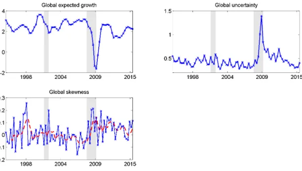
Figure 1.4: Global measures of risks. Shown are the three cross-sectional measures of global growth prospects. For global skewness, I also present a 4-quarter trailing average on the dashed line for ease of visual representation.
prospects of the variable being forecasted. Similar to how the median forecast can serve as the expectation of growth rate, the extent of how dispersed the predictions are can serve as the proxy for variance. Moreover, if one notes a pronounced asymmetry in the distribution of predictions in that a fraction of respondents are making very low (or very high) predictions, then one may in-fer that there are some beliefs that the growth rate can tank significantly (or boost significantly), while there still prevails non-extreme beliefs about growth. Analogously, a negatively (or posi-tively) skewed distribution of macroeconomic prospects indicates there are some chances of left-tail (or right-left-tail) events while the remaining mass of the distribution is at the non-extreme part of the domain. Hence, our cross-sectional skewness of forecasts can arguably be interpreted as a measure of skewness risk about the macroeconomic prospects.
dis-plays an interesting pattern a number of quarters before the recessions. What we can observe is that global skewness tends to be low and negative a number of quarters before the onset of each recession. Intuitively, this means that a fraction of forecasters makes significantly pessimistic pre-dictions relative to the non-pessimistic crowd at periods before a recession begins. When a bad event actually realizes, most of the survey respondents revise their predictions downward, so that the skewness of the distribution is no longer low. It is precisely this dynamic that I believe cap-tures important time-series information about global macroeconomic risks.
Data on personal consumption and population are mostly from national sources and have been downloaded through Datastream. These data include: Federal Statistical Office of Germany, State Secretariat for Economic Affairs of Switzerland, Cabinet Office of Japan, Australian Bu-reau of Statistics, Statistics New Zealand and Statistics Norway. World Bank and IMF Interna-tional Financial Statistics have been also used for population data.
Foreign exchange data are obtained primarily from Thomson Reuters through Datastream. I obtain foreign exchange spot rates and 3-month forward rates on 33 currencies from Thom-son Reuters: United Kingdom, Japan, New Zealand, Australia, Sweden, Switzerland, Norway, Canada, South Africa, Singapore, Denmark, Euro, Austria, Belgium, Finland, France, Germany, Greece, Italy, Netherlands, Portugal, Spain, Ireland, South Korea, Czech Republic, Hungary, India, Malaysia, Mexico, Philippines, Poland, Taiwan, and Thailand. However, the data I have from Thomson Reuters only go back to the end of 1996, so for the period of 1995 through the third quarter of 1996 I use the 3-month interest rates and the spot rates for the major and Euro-joining currencies: United Kingdom, Japan, New Zealand, Australia, Sweden, Switzerland, Nor-way, Canada, South Africa, Singapore, Denmark, Austria, Belgium, Finland, France, Germany, Greece, Italy, Netherlands, Portugal, Spain, and Ireland. The sample period differs for different currencies either because of foreign exchange regimes, unreliable volatile periods, or data unavail-ability. The details about the foreign exchange data that I use can be found in Table A.3 in the Appendix.
1.4 Empirical Results
1.4.1 Predictive Regressions of Currency Returns
A common approach to understand the currency market is to study the returns to the carry trade. In practice this trading strategy involves taking long positions in currencies with high forward discount and taking short positions in those with low forward discount. This is roughly equivalent to forming long-short portfolios based on the aforementioned interest rate differentials, given that the covered interest rate parity approximately holds.
Based on the ordering of the forward discount, which is defined as the difference between the log forward ratefti and the log spot ratesit, I separate currencies into usually five buckets from the highest to the lowest. For exercises that restrict the investable set of currencies to, a smaller number of currencies, say the G10, then I separate them into three buckets instead. The dynamic strategy means that I take long positions in the currencies in the high bucket and short positions in the currencies in the low bucket, while re-balancing the portfolio every quarter based on the sorting of currencies. For the static strategy, I instead form a static portfolio based on the time series average of the forward discount for each currency. As an example with the most actively traded currencies in the world, the static strategy would involve taking long positions on the Australian dollar, New Zealand dollar, and Norwegian Krone, while taking short positions on the Deutsche Mark (soon replaced by the Euro), Swiss Franc, and Japanese Yen. The predictive re-gression exercise is to regress the next-quarter carry trade returns onto one or more of our global measures of risks Xt:
xrt+1=α+βXt+εt+1 (1.28)
wherexrt+1 indicates the return on the carry trade strategy from time tto the next quarter t+ 1, which consists of a long position in the high bucket and a short position in the low bucket. The currency excess return on a single foreign exchange rate iis defined as xrti+1 =sit+1−fti, and the portfolio return on a particular bucket is the average of the individual excess return xrti+1 for the currencies in the bucket. For the period before 1996.Q4, in which I use bonds data, the excess returns on the currencyiare defined as xrit+1 = iti −iU St + ∆st+1 and the forward discount is defined asf dit=iit−iU St .
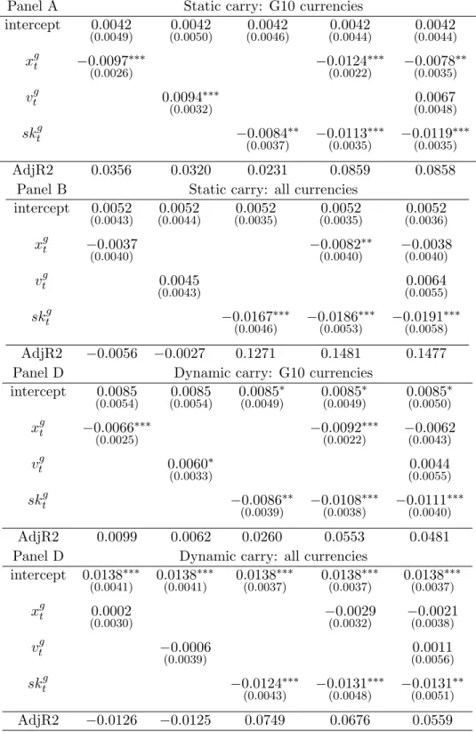
stan-Panel A Static carry: G10 currencies
intercept 0.0042 0.0042 0.0042 0.0042 0.0042 (0.0049) (0.0050) (0.0046) (0.0044) (0.0044)
xgt −0.0097∗∗∗ −0.0124∗∗∗ −0.0078∗∗
(0.0026) (0.0022) (0.0035)
vgt 0.0094∗∗∗ 0.0067
(0.0032) (0.0048)
skgt −0.0084∗∗ −0.0113∗∗∗ −0.0119∗∗∗ (0.0037) (0.0035) (0.0035) AdjR2 0.0356 0.0320 0.0231 0.0859 0.0858
Panel B Static carry: all currencies
intercept 0.0052 0.0052 0.0052 0.0052 0.0052 (0.0043) (0.0044) (0.0035) (0.0035) (0.0036)
xgt −0.0037 −0.0082∗∗ −0.0038
(0.0040) (0.0040) (0.0040)
vtg 0.0045 0.0064
(0.0043) (0.0055)
sktg −0.0167∗∗∗ −0.0186∗∗∗ −0.0191∗∗∗ (0.0046) (0.0053) (0.0058) AdjR2 −0.0056 −0.0027 0.1271 0.1481 0.1477 Panel D Dynamic carry: G10 currencies
intercept 0.0085 0.0085 0.0085∗ 0.0085∗ 0.0085∗ (0.0054) (0.0054) (0.0049) (0.0049) (0.0050)
xgt −0.0066∗∗∗ −0.0092∗∗∗ −0.0062 (0.0025) (0.0022) (0.0043)
vtg 0.0060∗ 0.0044
(0.0033) (0.0055)
sktg −0.0086∗∗ −0.0108∗∗∗ −0.0111∗∗∗ (0.0039) (0.0038) (0.0040) AdjR2 0.0099 0.0062 0.0260 0.0553 0.0481 Panel D Dynamic carry: all currencies
intercept 0.0138∗∗∗ 0.0138∗∗∗ 0.0138∗∗∗ 0.0138∗∗∗ 0.0138∗∗∗ (0.0041) (0.0041) (0.0037) (0.0037) (0.0037)
xgt 0.0002 −0.0029 −0.0021
(0.0030) (0.0032) (0.0038)
vtg −0.0006 0.0011
(0.0039) (0.0056)
sktg −0.0124∗∗∗ −0.0131∗∗∗ −0.0131∗∗ (0.0043) (0.0048) (0.0051) AdjR2 −0.0126 −0.0125 0.0749 0.0676 0.0559
dardize all global measures so that each has a mean of 0 and a standard deviation of 1. Panels A and B show the results for the static carry, and panels C and D show for the dynamic carry. Panels A and C present the results for portfolios formed using the G10 currencies, one of which is the Euro which replaced the Deutsche Mark in 1999. Panels B and D correspond to port-folios formed using all 33 currencies, in which the set of currencies being considered is chang-ing through time (See Table A.3 in Appendix). One can observe that the static carry trade re-turns based on the major currencies loads significantly on the global expected growth and global skewness with a negative sign and loads positively on global uncertainty, given the regression is done separately. If all three regressors are used altogether, then global expected growth and global skewness remain significant predictors of the carry trade returns. Moving onto the sec-ond panel, we can see that global uncertainty is no longer a significant predictor of the returns. Global skewness remains a reliably significant predictor of carry trade returns, while the loadings on global expected growth is not particularly significant. Likewise, the bottom panels C and D on the dynamic carry trade shows that the signs are consistent with those in the top panels A and B.
The economic magnitude of global conditional skewness is large. For the case of the dynamic carry trade based on a large set of currencies regressed on all three global measures, the loading on global skewness is -0.0131. Since my global measure is standardized, the coefficient suggests that a one standard deviation decline in global skewness indicates a rise in 5.24% risk premium per annum. Many of the other regressions suggest a per annum effect of at least 4%. Therefore, global conditional skewness risk appears to contribute to the time-variation in the carry risk pre-mium with large economic significance.
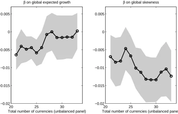
20 25 30 −0.02
−0.015 −0.01 −0.005 0 0.005
Total number of currencies (unbalanced panel)
β on global expected growth
20 25 30
−0.02 −0.015 −0.01 −0.005 0 0.005
Total number of currencies (unbalanced panel)
β on global skewness
Figure 1.5: Estimated beta loadings for different sets of currencies. Above are based on the dy-namic carry portfolio. Estimated βs and their 90% confidence intervals are shown. We have an unbalanced panel of currencies, so the number of currencies changes over time.
becomes stronger in describing a larger set of currencies in the world, which includes not just the major currencies but also a number of emerging market currencies. On the contrary, global ex-pected growth loadings become less negative as we consider a larger number of currencies. Hence we can argue that global expected growth has less predictive power in explaining the risk premia for a wider universe outside of the G10 currencies.
The negative loadings on global conditional expected growth and global conditional skewness inform us about the time-varying compensation for risk in the currency risk premium. When global conditional expected growth is low, the currency risk premium on the carry trade portfolio is high, meaning that there is a large risk premium arising from pessimistic prospects on global expected growth. Similarly, when global conditional skewness is low, or negative, the carry trade offers a high risk premium due to the perception of a negatively skewed distribution of global prospects, i.e., a high chance of a very significant downturn in the global economy. Conditional on such cases, the carry trade portfolio is considered risky, thus offering a high expected return.
when the recent crisis period is excluded. I define the recent crisis period consistent with the cor-responding NBER recession, i.e., the fourth quarter of 2007 through the second quarter of 2009. Upon excluding 7 quarters of this period, I repeat the above exercise and find that carry trade returns load significantly on global conditional skewness (see Table A.4 in Appendix). I uncover that global conditional skewness has strong predictive ability for explaining the currency markets even during normal periods. This is a distinct feature from the disaster literature, as one might expect negative skewness to be only about the possibility of a very bad event. Instead, global skewness continues to explain next period currency returns in normal times.
The loading on global uncertainty merits some discussion as the literature has emphasized the role of volatility in explaining asset returns. From various regression exercises, I conclude that the direction of the predictive ability of global uncertainty appears consistent with the literature but not statistically strong in our context. The economic story of a positive loading is that when global uncertainty is perceived to be high, the carry trade portfolio tends to yield high expected excess returns, meaning that there is a large risk premium when global uncertainty is ex ante high. This is consistent with the argument that when agents expect high economic uncertainty, they require high compensation for investing those risky currencies. As noted before, however, the statistical significance of the loading on the second moment is not very pronounced. If all three regressors are included on the right hand side of the regression, the coefficient on global uncertainty is never statistically different from zero. Although global economic uncertainty does have explanatory power in currency returns, it is usually subsumed by the other moments. Note that global conditional skewness contains the information about the direction of the risks, in that a negative skewness is very different from a positive value. Hence, we may argue that skewness contains information about whether the impending uncertainty is good or bad. Since skewness effectively informs the sign of the uncertainty, the role that the second moment can play is rela-tively diminished in explaining returns. Given the relarela-tively weaker explanatory power of global uncertainty, for subsequent analyses I exclude the results for it.
Switzer-land and China. The results are presented in Table A.5. I have alternatively tried an aggrega-tion method of taking the average weighted by each country’s GDP share. The results are in Ta-ble A.6. These robustness exercises generally convey a consistent message that global expected growth and global skewness seem to have predictive ability in explaining carry trade returns.
I further show predictive regressions using alternative measures of skewness in Table A.7. I denote the component of global conditional skewness that is not explained by global expected growth assktg,+. In other words, I regress global skewness onto global expected growth xgt and take the residuals that are not explained by xgt. The first and third columns show that this mea-sure still significantly predicts carry trade returns. The second and fourth columns use the alter-native measure that is constructed as p3
skgt ×pvtg. It measures the third moment raised to the power of one third and captures the direction of the uncertainty. I find evidence that this mea-sure is also a significant predictor of the carry trade returns, which is consistent with the equity return results shown in Colacito, Ghysels, Meng, and Siwasarit (2016).
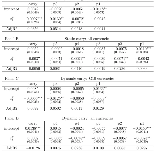
We may take a closer look at the carry trade regressions by examining the individual portfo-lios. Recall that carry trade is a high minus low strategy, i.e., it takes a long position in the high portfolio and takes a short position in the low portfolio. What we can instead study is to look at the returns on the high and low portfolios as well as the intermediate portfolios. We can take the time series of the returns on each portfolio, regress them onto our global measures of risks and compare the loadings across the portfolios.
Table 1.4 presents the results of regressing the individual portfolio returns onto global con-ditional skewness. The first column repeats the loadings on global skewness for reference, while the latter columns correspond to the high bucket portfolio, the middle, and the low, respectively. One can observe that the beta coefficients are negative and statistically significant for the high and medium portfolio, while the loading for the low portfolio is close to zero. A similar pattern holds in the case of the dynamic trading strategy.
port-Panel A Static carry: G10 currencies
carry p3 p2 p1
intercept 0.0042 −0.0020 −0.0051 −0.0118∗∗ (0.0046) (0.0068) (0.0045) (0.0054)
skgt −0.0084∗∗ −0.0093∗∗ −0.0098∗∗∗ 0.0005 (0.0037) (0.0038) (0.0033) (0.0044) AdjR2 0.0231 0.0202 0.0513 −0.0126
Panel B Static carry: all currencies
carry p5 p4 p3 p2 p1
intercept 0.0052 −0.0002 −0.0018 −0.0037 −0.0075 −0.0110∗∗∗ (0.0035) (0.0047) (0.0053) (0.0039) (0.0048) (0.0039)
skgt −0.0167∗∗∗ −0.0155∗∗∗ −0.0093∗∗∗ −0.0033 −0.0046 0.0026 (0.0046) (0.0050) (0.0030) (0.0056) (0.0040) (0.0029) AdjR2 0.1271 0.0851 0.0433 −0.0049 0.0027 −0.0068
Panel C Dynamic carry: G10 currencies
carry p3 p2 p1
intercept 0.0085∗ 0.0008 −0.0065 −0.0133∗∗ (0.0049) (0.0064) (0.0048) (0.0055)
skgt −0.0086∗∗ −0.0096∗∗ −0.0094∗∗ 0.0004 (0.0039) (0.0037) (0.0038) (0.0042) AdjR2 0.0260 0.0244 0.0371 −0.0126
Panel D Dynamic carry: all currencies
carry p5 p4 p3 p2 p1
intercept 0.0138∗∗∗ 0.0045 −0.0021 −0.0055 −0.0073 −0.0150∗∗∗ (0.0037) (0.0049) (0.0044) (0.0048) (0.0047) (0.0044)
skgt −0.0124∗∗∗ −0.0133∗∗∗ −0.0045 −0.0082∗∗ −0.0066 0.0004 (0.0043) (0.0045) (0.0042) (0.0038) (0.0041) (0.0028) AdjR2 0.0749 0.0772 −0.0014 0.0333 0.0132 −0.0125
Panel A Static carry: G10 currencies
carry p3 p2 p1
intercept 0.0042 −0.0020 −0.0051 −0.0118∗∗ (0.0049) (0.0069) (0.0048) (0.0053)
xgt −0.0097∗∗∗ −0.0130∗∗ −0.0072∗ −0.0042 (0.0026) (0.0054) (0.0036)
AdjR2 0.0356 0.0514 0.0218 −0.0041
Panel B Static carry: all currencies
carry p5 p4 p3 p2 p1
intercept 0.0052 −0.0002 −0.0018 −0.0037 −0.0075 −0.0110∗∗∗ (0.0043) (0.0053) (0.0054) (0.0041) (0.0047) (0.0038)
xgt −0.0037 −0.0071 −0.0091∗∗ −0.0039 −0.0071∗∗ −0.0043 (0.0040) (0.0054) (0.0043) (0.0035) (0.0032) (0.0026) AdjR2 −0.0056 0.0081 0.0410 −0.0019 0.0236 0.0033
Panel C Dynamic carry: G10 currencies
carry p3 p2 p1
intercept 0.0085 0.0008 −0.0065 −0.0133∗∗ (0.0054) (0.0066) (0.0052) (0.0053)
xgt −0.0066∗∗∗ −0.0125∗∗ −0.0050 −0.0069∗ (0.0025) (0.0052) (0.0038) (0.0037) AdjR2 0.0099 0.0502 0.0013 0.0129
Panel D Dynamic carry: all currencies
carry p5 p4 p3 p2 p1
intercept 0.0138∗∗∗ 0.0045 −0.0024 −0.0055 −0.0077 −0.0150∗∗∗ (0.0041) (0.0053) (0.0044) (0.0051) (0.0048) (0.0041)
xgt 0.0002 −0.0063 −0.0075∗∗ −0.0059 −0.0057 −0.0074∗∗ (0.0030) (0.0048) (0.0034) (0.0035) (0.0038) (0.0030) AdjR2 −0.0126 0.0075 0.0238 0.0109 0.0085 0.0297
folios. We can conclude that the the returns on the higher forward-discount portfolios load more negatively on global skewness, thus explaining the high minus low carry strategy that I showed earlier.
The results for regressing on global expected growth are presented in Table 1.5. Although we can find a similar monotonic pattern if the set of currencies was limited to the G10 currencies, this is not necessarily the case if we include many other currencies. The loadings on the ’high’ bucket are not significantly negative and are not necessarily larger in magnitude than the others. Therefore, I argue that global conditional skewness seems to be the stronger predictor that pro-duces a monotonic pattern when comparing across the portfolios formed on the forward discount.
In summary, the empirical results show that my measures of global expected growth and global skewness have predictive ability in explaining the carry trade returns. In particular, the explanatory power of global skewness becomes more robust as I include a larger number of cur-rencies.
Before I conclude this section, I address the following concern about robustness with regards to whether I have sufficient analyst coverage in constructing a robust measure of global skewness. To be more precise, I need enough number of analysts projecting forecasts for a given country and also for a sufficient number of countries, over which I aggregate. To justify this I conduct the following Monte Carlo exercise. Taking the data of quantile-based skewness in forecasts for each country as given, for every point in time tand for every countryc I generate Ic,t random
ana-lysts’ forecasts from the skewed distribution based on Matlab’s random number generation from a Pearson system that intakes the observed skewness2. I then calculate the quantile-based skew-ness of on the randomly generatedIc,t analysts’ forecasts. Repeat this for every country to
con-struct the global measure of skewness and then repeat this for all t. Run a time-series regression of the dynamic carry returns with the set of all available currencies onto the randomly generated measure of global skewness to obtain an estimate of the loading. Repeat this for a 1,000 simula-tions and then obtain the distribution of the estimated loading. The 90% confidence interval of the estimated loading is (-0.0142, -0.0015884), indicating that the Monte Carlo simulation exer-cise indicates my given data of analyst coverage is sufficient in terms of justifying the predictive
2
regression result.
1.4.2 Robustness
In order to provide evidence that global skewness is indeed a robust predictor, I consider a few variables known to have explanatory power for the foreign exchange market. The first variable I consider is the innovations to liquidity ∆liquidityt, where liquidity is proxied by the negative of
the TED spread (LIBOR minus the 3-month Treasury Bill rate), retrieved from the FRED. The literature has documented that changes in liquidity can help predict subsequent carry trade re-turns as shown in Brunnermeier, Nagel, and Pedersen (2009) and Bakshi and Panayotov (2013).
Table 1.6 shows the results when next-quarter carry trade returns are regressed jointly on global skewness and the liquidity innovation. The predictive ability of the carry trade returns remains robust, when the liquidity channel is controlled for.
I also consider two other explanatory variables that are contemporaneous instead of lagged. I consider the innovations in foreign exchange volatility ∆fxvolt+1, in which foreign exchange
volatility is defined as
fxvolt=
1 9
9 X
i=1 v u u t
X
τ∈quartert
(∆sdailyτ )2
(1.29)
fori∈ {G10 currencies}. This variable is in line with Menkhoff, Sarno, Schmeling, and Schrimpf (2012) who find that the long-end of the carry trades tends to deliver low returns during periods of unexpected high global FX volatility. Following their argument, unexpected volatility proxy should be a contemporaneous variable instead of a predictor, namely that the timing of unex-pected volatility ∆fxvolt+1 is consistent with the timing of the carry trade returnscxrt+1.
Another explanatory variable of interest is the growth rate of a commodity index called the Commodity Research Bureau BLS Spot Index, retrieved from Datastream. Despite the proposed relationship between commodity prices and foreign exchange rates, there is mixed evidence of whether commodity prices can predict future foreign exchange rates (Chen, Rogoff, and Rossi (2010)). I instead consider the contemporaneous innovation ∆commodt+1.
by a large extent. In addition, correlations among the covariates likely change the coefficient es-timates. Nonetheless, global skewness appears to be a statistically significant predictor of future carry trade returns.
A similar exercise for the carry based on the G10 currencies is reported in the Appendix (Ta-ble A.8). The predictive power of global skewness given a control for the liquidity proxy remains significant. Given the control for the role of FX volatility or commodity, the role for global skew-ness is statistically weak, but the lack of power is due to the high R2 arising from the contempo-raneous variables.
Panel A: dynamic Panel B: static
intercept 0.0136∗∗∗ 0.0132∗∗∗ 0.0130∗∗∗ 0.0049 0.0043 0.0037 (0.0035) (0.0036) (0.0040) (0.0033) (0.0032) (0.0037)
sktg −0.0131∗∗∗ −0.0103∗∗ −0.0102∗∗∗ −0.0173∗∗∗ −0.0137∗∗∗ −0.0130∗∗∗ (0.0043) (0.0042) (0.0033) (0.0046) (0.0041) (0.0034)
∆liquidityt 2.8612∗∗∗ 2.5495∗∗
(0.7725) (1.1047)
∆fxvolt+1 −0.9988 −1.4434∗∗∗
(0.6031) (0.4860)
∆commodt+1 0.1754 0.2957∗∗∗
(0.1192) (0.0973)
AdjR2 0.1511 0.1955 0.1277 0.1773 0.3590 0.2772 Table 1.6: Regressions of carry trade returns onto global skewness and other explanatory vari-ables. Above carry trades are formed based on all available set of currencies. The left three columns are based on the dynamic carry, and the right three columns are based on the static carry. ∆liquiditytis a lagged innovations to liquidity, defined as the minus of TED spread.
∆fxvolt+1 is a contemporaneous innovations to the foreign exchange volatility constructed from the G10 currencies. ∆commodt+1 is a contemporaneous growth rate of the CRB BLS Spot In-dex.
1.4.3 Trading Conditional on Global Skewness
2000 2005 2010 2015 0.1
0.2 0.3 0.4 0.5 0.6 0.7 0.8
Dynamic carry based on G10
Carry New
2000 2005 2010 2015 0
0.1 0.2 0.3 0.4
Cumulative returns
Static carry based on G10
Carry New
2000 2005 2010 2015 0.2
0.4 0.6 0.8 1 1.2 1.4
Dynamic carry based on all currencies
Carry New
2000 2005 2010 2015 0.2
0.4 0.6 0.8 1 1.2
Cumulative returns
Static carry based on all currencies
Carry New