MODELING NON-LINEARITY IN RELIGIOSITY’S RELATIONSHIPS TO PREMARITAL SEXUAL ATTITUDES AND BEHAVIORS AMONG ADOLESCENTS AND YOUNG
ADULTS
George M. Hayward
A thesis submitted to the faculty at the University of North Carolina at Chapel Hill in partial fulfillment of the requirements for the degree of Master of Arts in the Department of Sociology
in the College of Arts and Sciences.
Chapel Hill 2016
Approved by:
Lisa D. Pearce
Samuel P. Morgan
ABSTRACT
George M. Hayward: Modeling Non-linearity in Religiosity’s Relationships to Premarital Sexual Attitudes and Behaviors among Adolescents and Young Adults
(Under the direction of Lisa D. Pearce)
Using data from three waves of the National Study of Youth and Religion, this paper
examines the relationships of religiosity with premarital sexual attitudes and behaviors for
adolescents and young adults. Following past research that shows evidence for non-linear
relationships between these variables, particularly among the highly religious, this paper
explicitly compares three functional forms of these relationships. The results show that nearly all
of these relationships are best defined when non-linearity in the functional form is accounted for.
That is, a linear-only approach often obscures large differences between the most religious
individuals and their less-religious peers. These findings hold for both age groups of interest,
suggesting that religious influence is markedly non-linear for these outcomes from adolescence
into young adulthood. Further, these findings lay the groundwork to revisit religious influence
across other domains and to test whether religiosity has been conceptualized and modeled in the
ACKNOWLEDGEMENTS
The author would like to thank Roger Finke for his guidance and encouragement at the
early stages of this paper. The author would also like to thank Lisa Pearce, Phil Morgan, and
Michael Shanahan for helpful suggestions throughout the development of this paper. This
research received support from the Population Research Training grant (T32 HD007168) and the
Population Research Infrastructure Program (P2C HD050924) awarded to the Carolina
Population Center at The University of North Carolina at Chapel Hill by the Eunice Kennedy
Shriver National Institute of Child Health and Human Development. The National Study of
Youth and Religion, http://youthandreligion.nd.edu/, whose data were used by permission here,
was generously funded by Lilly Endowment Inc., under the direction of Christian Smith, of the
Department of Sociology at the University of Notre Dame and Lisa Pearce, of the Department of
TABLE OF CONTENTS
LIST OF FIGURES ... vi
LIST OF TABLES ... vii
INTRODUCTION ... 1
THEORY AND BACKGROUND ... 3
Empirical Studies with Apparent Threshold Effects ... 6
Identifying the “Highly Religious” ... 10
Life Course Variation ... 11
Conceptualizing the Optimal Form of Religious Influence ... 13
DATA AND METHODS ... 16
Dependent Variables ... 17
Independent Variables ... 19
Analytic Strategy ... 22
RESULTS ... 24
DISCUSSION ... 31
APPENDIX 1: CODING OF RELIGIOUS INDEX ... 36
APPENDIX 2: FIGURES AND TABLES ... 39
LIST OF FIGURES
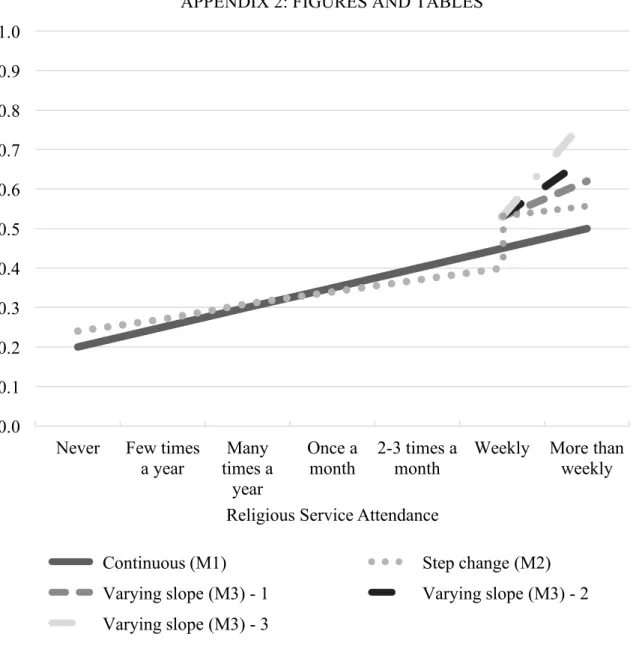
Figure 1 – Functional Forms of the Relationship between Religious Service
Attendance and the Odds of a Hypothetical Outcome...39
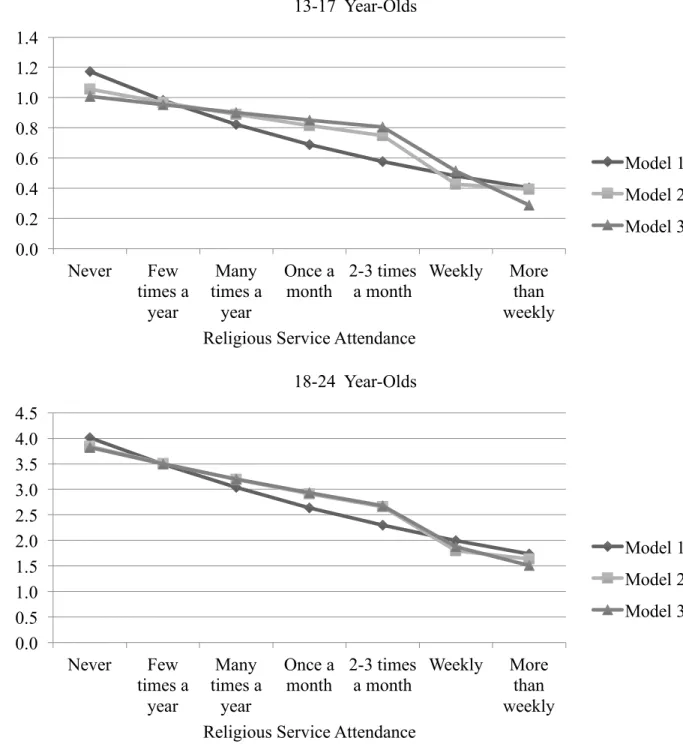
Figure 2 – Expected Number of Sexual Partners for 13-17 Year-Olds and 18-24
LIST OF TABLES
Table 1 – Functional Forms of the Relationship between Religious Attendance
and a Hypothetical Outcome using Logistic Regression...41
Table 2 – Descriptive Statistics for All Variables...42
Table 3 – Logistic Regression Models Predicting Favorable Attitudes toward Abstinence before Marriage...43
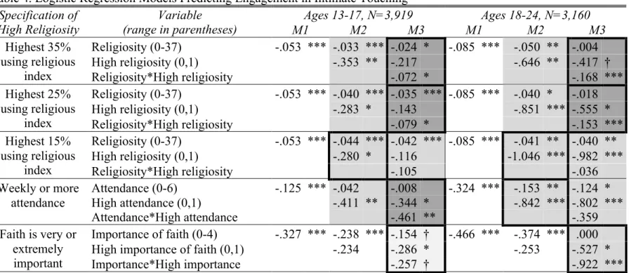
Table 4 – Logistic Regression Models Predicting Engagement in Intimate Touching...44
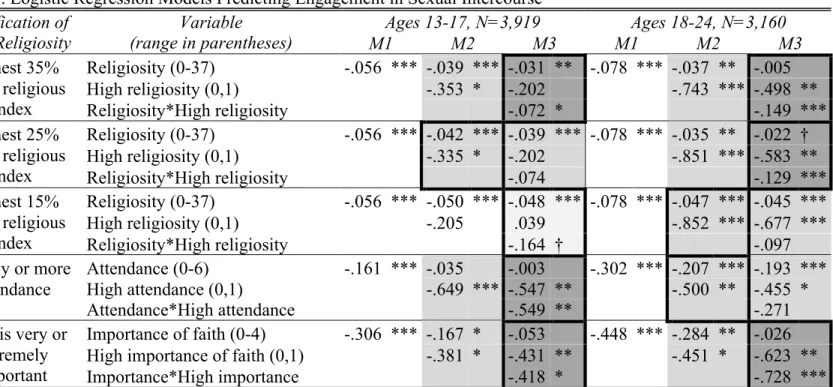
Table 5 – Logistic Regression Models Predicting Engagement in Sexual Intercourse...45
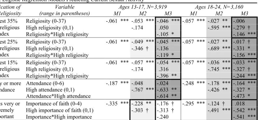
Table 6 – Logistic Regression Models Predicting Current Sexual Activity...46
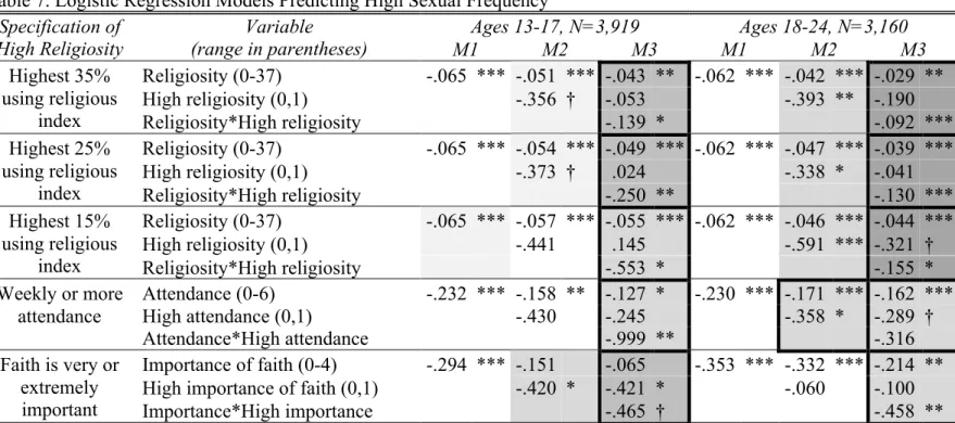
Table 7 – Logistic Regression Models Predicting High Sexual Frequency...47
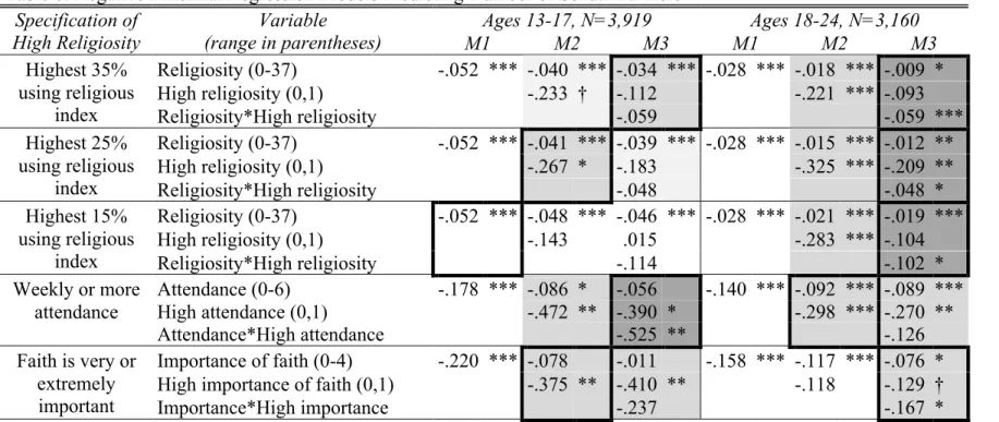
Table 8 – Negative Binomial Regression Models Predicting Number of Sexual Partners...48
INTRODUCTION
Risky sexual activity during adolescence has attracted substantial scholarly attention. The
prevalent consequences of risky sexual behavior, such as unintentional pregnancies and sexually
transmitted diseases, point to the importance of this issue across disciplines and the need for
further research. In 2008, for example, about 82 percent of pregnancies for females ages 15 to 19
were unintended – totaling about 612,000 pregnancies – and approximately 36 percent of those
pregnancies ended in abortion (Finer and Zolna 2014). Additionally, 10 million sexually
transmitted infections (STIs) are contracted in the United States each year among adolescents
and young adults ages 15 to 24 (Centers for Disease Control and Prevention 2013). These STIs,
in turn, can lead to health issues, infertility, ectopic pregnancy, and death, while costing the
healthcare system approximately $16 billion in direct medical costs (Centers for Disease Control
and Prevention 2013, 2014). Despite these risks, the majority of adolescents become sexually
active between the ages of 15 and 21. In this span of six years, the percentage of adolescents who
have engaged in sexual intercourse increases from 25 to 85 percent (Mosher, Chandra, and Jones
2005).
Among the factors associated with the transition to sexual activity, researchers have
given considerable attention to religion. Numerous studies have shown religious beliefs and
involvement to play a major role in influencing sexual attitudes and behaviors. For example,
religious youth are more likely to believe that sex should be reserved for marriage, to become
sexually active at later ages, to pledge abstinence until marriage, and to have fewer sex partners
these findings, though, shows that youth are not all influenced by religion in the same way. In
fact, how religiosity is measured often presupposes that there is a linear relationship between
religiosity and sex-related dependent variables; that is, as religiosity increases, sexual attitudes
become more conservative and sexual behaviors decrease accordingly. If this relationship is
non-linear, though, many existing findings on the relationship between religion and sex, and perhaps
other dependent variables, may be missing an important caveat about religious influence:
religion may have a markedly different influence, or no influence, on some individuals, but a
rather large influence on others, creating the appearance of linearity when averaged together.
Unfortunately, little attention has been given to the functional forms of these
relationships and social relationships more generally. Montez, Hummer, and Hayward
(2012:334) argue that "research on the functional forms of sociodemographic relationships,
while an often-ignored issue, is fundamental for understanding those relationships." These
authors test 13 different forms of the relationship between educational attainment and mortality,
and conclude that such research not only deepens our empirical understanding of such
relationships, but also provides the groundwork for theory building and elaboration. Thus, an
in-depth, theory-driven examination on the forms of the relationships between religion and sex can
greatly advance our understanding of this well-documented relationship.
The aim of this paper is to take one particular cluster of outcomes - sexual attitudes and
behaviors - and to test whether previous research has modeled religiosity in the most appropriate
way to define these relationships. Specifically, this research is guided by the following three
research questions: (1) What are the optimal forms of the relationships between religious
variables and outcomes regarding sexual attitudes and behaviors? (2) Do the optimal forms of
statistical and substantive interpretations of these relationships change when different forms are
accounted for? I hypothesize that religiosity will not be related to such outcomes linearly, as it is
often measured in past research, but that a certain amount of religiosity is needed before religious
influence becomes recognizable. A modeling approach that allows for this potential non-linearity
may better illustrate religion's relationship to sexual attitudes and behaviors than continuous
measures. I also hypothesize that the importance of form will vary across adolescence and young
adulthood. Specifically, I expect that non-linear forms of these relationships will be more
apparent during young adulthood than adolescence.
If these hypotheses are confirmed, the findings will suggest that nominal involvement
with religion may not be enough for adolescents to be influenced by it. With so many prosocial
outcomes associated with religiosity, such as lower levels of substance use, crime, and violence
(Smith and Faris 2002), improved mental and physical health behaviors (Dew et al. 2008;
Nooney 2005; Wallace and Forman 1998), and heightened levels of volunteerism and
community service (Smith and Faris 2002; Youniss, McLellan, and Yates 1999), these findings
would also lay the groundwork for re-analysis of many outcomes associated with religion. It
could be that other variables, too, for example, are related to religiosity in non-linear ways and
that the protective effects of religion that this literature suggests may thus be overstated for some
youth and understated for others. To clarify these relationships in future research, scholars may
benefit from theorizing about functional forms and using non-linear modeling techniques to
supplement or replace standard linear ones.
THEORY AND BACKGROUND
An underlying assumption in much of the sociological research on religion is that its
interval-level variables in linear regression. It is unclear whether this convention has materialized
because of practicality, the desire for parsimoniousness, or from a theoretical expectation that
religion influences individuals equally. Regardless, there are theoretical reasons to believe that
religious influence can affect individuals in radically different ways. For example, Smith
(2003:19) theorizes about nine "distinct but connected and potentially reinforcing factors" that
explain religious influence among adolescents. These nine factors fall under three broad
dimensions of moral order, learned competencies, and social and organizational ties. It can be
argued, however, that these mechanisms for religious influence are far less likely to apply to
nominally religious youth than for those who are deeply religious. Compared to those who are
more religiously active, an adolescent who sporadically practices religion will likely be
disadvantaged when it comes to internalizing moral directives, serving in religious leadership
positions, finding consistent peer and adult role models, and benefiting from network closure and
adult supervision. On the other hand, it is likely that the most embedded youth benefit from the
overlap between the nine proposed factors, and thus benefit also from their mutually reinforcing
influences on one another. In other words, as one becomes more religious, the influence of
religion may become substantially more recognizable in one's life.
There is also reason to suspect, following identity theory (Stryker 1968), that religion
only motivates attitudes and behaviors insofar as it has become part of a salient self-concept
within an individual. Those who place religion highly in their identity hierarchy may invoke
religious norms, teachings, and behaviors in a manner unlike those for whom religion is at the
bottom of the salience hierarchy. Presumably, these are the people most likely to exhibit some
congruency between their religious convictions, attitudes, and behaviors. This congruency may
religion to be wary of what he calls "the congruence fallacy," which is the often erroneous
assumption that religious individuals have tightly knit and integrated beliefs systems, that they
act congruently with their beliefs and values, and that they can readily access and apply their
religious beliefs and values across contexts. That kind of consistency, Chaves (ibid.) argues, is
rare. It is the exception rather than the rule. Unfortunately, he believes that researchers often
interpret research findings "in ways that presuppose a congruence that we know is not generally
there" (2). If religious congruence is indeed rare, then religion should not be expected to have a
global influence on all of its practitioners. Rather, it would be more sensible to assume that it has
relatively trivial influences on most people and distinctively large influences on those who
somehow manage to integrate their beliefs, values, and behaviors into a congruent religious
identity.
Adding to this line of reasoning, highly religious individuals may have pronounced
mental schemas that have accumulated over time from social interactions and differential access
to religious materials (Johnson-Hanks et al. 2011). According to the theory of conjunctural
action, schemas and materials comprise structure, which is a patterning of social life. Structures
are reflected in identity, and within a structure an identity can be fortified. Importantly, the
theory states, "a schema will not generate an identity unless enacted, and behavior does not
create an identity unless it gives a self-schema material form. Identities are created and sustained
through the interaction of both schemas and materials" (ibid.:14). In other words, structure
provides the raw materials for identity formation, but individuals' choices, given their schemas
and materials, can reinforce or weaken their current identities. The contexts in which individuals
make these choices or take action are referred to as "conjunctures," and how these conjunctures
a "religious" manner, Chaves (2010) would likely refer to them as congruent. But this
congruency is rare, he argues. So it must be that many religious people do not resolve
conjunctures in a religious manner, but rather in ways that follow from non-religious schemas
and identities. Those most likely to act congruently, it seems, would be those with the most
salient schemas and identities, heightened access to religious materials, and the overlap of
Smith's (2003) nine factors that are comparable to a religious "structure" from the theory of
conjunctural action. It may be appropriate to assume, then, that religious influence would look
different for this group than for others who may be nominally affiliated with a religion but who
have little religious salience or commitment to it.
The theoretical arguments presented thus far support the idea that religious influence
should not be expected to operate monotonically across individuals. Rather, religious influence is
more likely to be minimal or modest for most individuals while dramatically stronger for those
highest in religiosity. In statistical models, a continuous, linear measure of religiosity would
obscure this contrast. While no study, to my knowledge, explicitly compares linear forms of
religious influence to non-linear alternatives across the same outcomes, the available empirical
evidence suggests that the optimal forms will indeed take non-linearity into account.
Empirical Studies with Apparent Threshold Effects
In a study of delinquency, risk behaviors, and constructive social activities among a
representative sample of twelfth graders, Smith and Faris (2002) use religious service attendance,
the importance of religion, and years of youth group involvement as ordinal variables in their
analyses. Interestingly, statistically significant relationships between these independent variables
and many of the dependent variables are limited to only those reporting the highest levels of
important, and, to a lesser extent, have attended youth group six or more years (all with respect to the baseline categories of no attendance, no religious importance, and no youth group
participation). The outcomes in this study include the onset to cigarette smoking, regular
smoking, age at first drunk experience, frequency of attending bars, frequency of drinking to get
drunk, use of illegal drugs, use of hard drugs, having smoked marijuana, and age at first
marijuana usage, among others. Surely, these outcomes are of great importance to parents,
educators, and policy-makers alike. Yet, interestingly, findings from this study suggest that
semi-religious youth (e.g., those who attend semi-religious services and youth group sporadically or find
religion just somewhat important) are not statistically different from the least religious youth
among these variables. Had the authors instead used continuous religion variables in these
analyses, their overall relationships might have appeared significant; however, this could have
resulted from the highly religious youth disproportionally biasing the estimates toward their own
outcomes (and toward statistical significance).
Continuing the examples from Smith and Faris (ibid.) above, the percentage of youth
who never drink to get drunk is 28 percent for weekly attenders but approximately 17 percent for
everyone else, regardless of how much they attend religious services. The same trend appears to
hold for the importance of religion, such that 30 percent of youth who consider religion to be
very important never drink to get drunk, while that percentage is approximately 16 percent for
everyone else, regardless of how important they think religion is.
Smith and Denton (2005), using ideal types of religiosity, investigate various outcomes
during adolescence and how they relate to religion variables. They notice stark differences
between highly religious youth and those only moderately involved in religion, and comment:
involvements by teens in religion usually prove indistinguishable in outcomes from those of teens who are completely disengaged from religion. Religious associations with more positive life outcomes generally appear to require teens reaching the level of religiosity of at least the Regulars to be statistically significantly different from the Disengaged. A modest amount of religion, in other words, does not appear to make a consistent difference in the lives of U.S. teenagers. It is only the more serious religious teens, the Regulars and Devoteds, whose outcomes are more consistently and significantly more positive than those of their entirely religiously Disengaged peers" (2005:232–233).
Despite this astute observation from their analysis of ideal types, the authors did not test whether
this same threshold effect could be captured using continuous variables, which are generally
more common in the sociology of religion.
In a follow-up study with the same adolescents as Smith and Denton (2005), Pearce and
Denton (2011) identify similar relationships among the “Abiders.” The authors classify youth
into five different religious mosaics: Abiders, Adapters, Assenters, Avoiders, and Atheists.
Among these, the Abiders report the highest levels of all institutionally related indicators of
religion. In regard to risk behaviors, Pearce and Denton note, “Abiders at the time of the first
survey [The National Study of Youth and Religion, Wave 1] stand apart from the other profiles,
with much lower levels of reported risk behaviors at the time of the second survey” (78). For
example, 69 percent of Abiders did not have sexual intercourse by Wave 2 of data collection,
compared to 41 percent, 41 percent, 38 percent, and 31 percent among the other profiles,
respectively. This suggests, again, that there is some unique contribution of religious influence
for those who are distinctively religious and for whom, in this case, fall within a particular
religious profile.
Regnerus and Elder (2003), after examining the relationship between religiosity and
problem behaviors of low-risk youth, suggest that “in terms of its efficacy, religiosity may be
less of an ordinal variable than a dichotomous one – the key distinction being the very religious
religion measures and problem behaviors. Unfortunately, the authors do attempt to model a
discontinuity of religious influence in their regression models; instead, they use their measures as
continuous variables that only provide one generalized effect of religious influence.
On the topic of sex and religion, Regnerus (2007) finds an apparent threshold for both
religious service attendance and religious salience. Regarding the latter, he states, “For religious
salience at age 18, we only see two clusters: there is no statistical difference in virginity status
among youth who say religion is fairly important, fairly unimportant, or not important at all.
Only those who say it’s very important stand out, at 56% percent (nonvirgins)” (120-121).
Although not expounded upon, religious service attendance has a nearly identical relationship for
those who attend weekly versus those who attend once a month, less than once a month, and
never. Regnerus (ibid.) later summarizes this when investigating the various denominations, and
states, “Religious influence on sexual decision making is most consistently the result of high
religiosity rather than certain religious affiliations” (161).
Despite the intriguing findings from these studies, there has yet to be an integrated study
of religious variables that attempts to model a potential threshold and that tests whether such a
model would serve as a useful conceptual and analytical framework. Given the apparent
thresholds of religiosity in the literature, and the grounding for such a threshold theoretically,
there is reason to believe that such an approach would be useful. This leads to the following
hypothesis:
H1: The relationships between religiosity and sexual attitudes and behaviors are
Identifying the “Highly Religious”
The question now remains: who should be considered the highly religious youth? From
the studies previously discussed, the threshold seems to vary. Smith and Faris (2002) find that
those who attend weekly or more (31 percent of youth), consider religion to be very important
(30 percent of youth), and have attended youth group six or more years (16 percent of youth)
stand out from their peers on many different outcomes using the Monitoring the Future data.
Smith and Denton (2005) categorize 8 percent of youth as "Devoted" and another 27 percent as
"Regulars." Combined, they represent 35% of youth with the National Study of Youth and
Religion (NSYR) data. Regnerus (2007) offers a few suggestions of his own, also using the
NSYR data. First, he states, "About one in every five teenagers, however, says that religion is
extremely important in shaping how they live their daily lives. These are what I call the 'truly devout.' Their patterns of behavior are often distinct, even from those (31 percent) who say that
religion is 'very important.' The same can be said for the 16 percent of youth who attend religious
services more than once a week, as opposed to once a week (24 percent) (2007:12)." Finally,
Pearce and Denton (2011) find the Abider religious profile, identified through latent class
analyses, to be distinct from the others, which represents between 20 and 22 percent of youth,
depending on the survey year.
In sum, “highly religious” youth could represent between 8 and 35 percent of youth,
depending on the age of respondents, outcome(s) of interest, and the subjective discernment
about the minimum level of religiosity needed to be "highly religious." Nevertheless, reasonable
estimates can be made from synthesizing these studies and their data. A strict estimate is that
approximately 15 percent of youth are "highly religious," because about this percentage of youth
more lenient boundary for high religiosity is about 35 percent of youth. This represents the
approximate percentage of youth who attend religious services weekly or more or consider
religion to be at least very important. This group closely aligns with the "Regulars" as defined by
Smith and Denton (2005), which represent 27 percent of youth who fit into the ideal type.
Combining this group with "Devoted" youth, the total increases to 35 percent. Over a wide range
of outcomes, these two categories of youth stand apart from less engaged and non-religious
teens, with Devoted teens seeming to be the most influenced by religion (ibid.). This leads to the
second hypothesis:
H2: Religiosity will function as a non-linear predictor of sexual attitudes and behaviors when the threshold between low and high religiosity distinguishes between 15 and 35
percent of youth as highly religious. Life Course Variation
Finally, life course variation must be considered for a thorough analysis of differences in
the measurement and modeling of religious variables. For example, if the forms of relationships
matter for statistical models and determining statistical significance, they may matter more or
less depending on respondents' stages in the life course. Especially during adolescence, the
difference of a few years between respondents could be monumental, and these differences may
be especially sensitive to measurement differences. Indeed, Smith and Denton (2005) discuss
that many adolescents view religion through the life course perspective. In interviews,
adolescents suggest that there are age appropriate scripts of what is typical for teens and adults,
with religion having a different relevance for each group. Some even make it clear that they only
expect religion to matter later in their lives. I speculate here that the most religious youth will be
times when religion may be most tempting to push off until later years. For example, if we
assume that most religions have proscriptions against premarital sexual activity, we would
expect "congruent" religious individuals to be most different from their peers when sexual
activity is both fairly common for their age group and a legitimate option for most individuals to
pursue (in terms of agency and age-appropriateness). In other words, religious differences in this
domain would be less noticeable among young adolescents because they are less sexually active,
have fewer sexually active peers, and presumably have less autonomy to pursue sexual interests.
At least two studies provide evidence that religious distinctions become more pronounced
throughout adolescence and the transition to young adulthood. First, Burdette and Hill (2009)
find that private religious activities "have stronger associations with sexual touching, oral sexual
behavior, and sexual intercourse as teens move throughout adolescence" (41). This follows from
their arguments that age may function as a proxy for religious socialization and that religious
variables become more precise as they increasingly reflect those of the individual rather than his
or her parents. This latter argument, in fact, is one of the primary findings of Pearce and Denton
(2011) and a key reason why some adolescents consider themselves more religious over time
despite decreases in religious service attendance. Second, in terms of absolute percentages,
Regnerus (2007) finds that highly religious youth tend to be increasingly different from their
peers in the percentage of nonvirgins over time. One additional consideration is the possibility
that the transition to sexual activity reduces religiosity. There is mixed evidence for this, as some
studies find no such relationship (Hardy and Raffaelli 2003; Meier 2003) while others do
(Regnerus and Uecker 2006; Uecker, Regnerus, and Vaaler 2007). If true, however, then
non-sexually-active older adolescents will be more religious, on average, than their sexually active
non-linear effects of religious influence on sex-related outcomes. This leads to the third and final
hypothesis:
H3: Threshold effects for religious variables and sexual attitudes and behaviors will be
more pronounced during young adulthood than during adolescence.
To date, too many studies have summarized religious influence with one global "effect"
for all respondents, neglecting the possibility that religious influence may depend on one's
current level of religiosity. To overcome this, scholars must theorize about the expected forms of
relationships and use appropriate statistical models to reflect those forms. Assumptions about
different forms, such as whether the relationships are linear, whether they plateau at a certain
point, or whether they increase exponentially, all produce different interpretations of these
relationships. Accordingly, if researchers' assumptions about the forms of these relationships are
inaccurate, they will be sub-optimally represented in statistical models. I am hypothesizing here,
for example, that a threshold of high religiosity exists in which religious influence becomes
substantially stronger among individuals. The functional forms worth investigating and testing
empirically, then, are those that allow for a change in religious influence upon crossing the "high
religiosity" threshold.
Conceptualizing the Optimal Form of Religious Influence
Many studies have identified negative relationships between religious variables and
measures of sexual activity using continuous measures for religion variables (Adamczyk 2009;
Adamczyk and Felson 2006; Barkan 2006; Burdette and Hill 2009; Hardy and Raffaelli 2003;
Lefkowitz et al. 2004; Regnerus 2007; Sheeran et al. 1993; Sinha, Cnaan, and Gelles 2007;
Thornton and Camburn 1989). However, for the reasons thus outlined, alternative forms of this
within these relationships. Specifically, forms should be tested that allow highly religious
individuals to be distinct from less religious individuals analytically. This can be accomplished
in at least two ways: 1) allowing for an additive effect of high religiosity and 2) allowing for both
an additive and a multiplicative effect high religiosity. Both of these alternatives will be tested
here and compared to conventional, continuous measures of religiosity. The equations for these
models are shown in Table 1 below, and Figure 1 graphically depicts how these equations may
be related to a hypothetical outcome. Table 1, and the explanations of each model, follow the
precedent set by Montez et al. (2012) in their analysis of functional forms.
Model 1: Continuous model. For this model, religious variables are specified as linear (e.g., coded with values such as 0-5 or 1-6). It is assumed that the influence of religiosity is the
same for every increase in religiosity, regardless of where that change occurs on the religiosity
continuum.
Model 2: Step change with constant slope. The first alternative model is specified such
that there is a step-change for the highly religious individuals compared to their counterparts.
With this approach, the influence of additional religiosity is the same for both groups (i.e., the
slope is the same), but the highly religious group gets a "boost," or additional (additive) effect of
religiosity, solely for being in the highly religious group. This effect is captured analytically
simply by adding a dummy variable to the model for high religiosity. Accordingly, this effect
remains constant for each additional increase of religiosity beyond the "high" threshold. Most
simply, this model allows the y-intercept of highly religious individuals to be different from
those with less religiosity. Theoretically, this is one way to capture the identity component of
religiosity, and it most closely approximates the “credentialist” perspective (Collins 1979) that
with mortality decline. In this case, high religiosity would signal entry into a group that opens
doors to additional religious socialization and that leads individuals to think of themselves as
being “religious.” It would not change the effect of religiosity beyond membership in this group,
but the group membership itself would have an effect.
Model 3: Step change with varying slope. The third approach builds on the second and
can be described as a step change with a varying slope. The step change from the previous model
remains the same: highly religious individuals receive an additional effect of religiosity solely
for being in the highly religious group. However, in this model, the influence of religiosity
beyond the high religiosity threshold is now allowed to have its own slope. This is accomplished by adding to the model an interaction term (for a multiplicative effect) between the continuous
linear variable for religiosity and the dummy variable for high religiosity. If this term is
significant, it indicates that the slope for the highly religious group differs from that of the group
with low religiosity. Theoretically, this form follows from the idea that once within the high
religiosity group, the impact of additional religiosity changes. As discussed previously, there are
reasons to believe that religiosity may have a fairly small impact on individuals until it becomes
a salient identity (Stryker 1968) or informs mental schemas (Johnson-Hanks et al. 2011). After
this point, additional embeddedness within religious communities will likely build upon and
reinforce existing religious identities (Smith 2003) while simultaneously heightening awareness
to the possibility of cognitive dissonance should one act irreligiously. If this is the case, it is not
only membership in the highly religious group that matters but also how religious one is within
that group.
For a comprehensive test of the hypotheses, these three models will be estimated for a
previous literature in several ways. First, to my knowledge, no analysis of these relationships has
heretofore explicitly examined nor compared alternative functional forms. Second, this study
examines functional forms among five different religious variables (three versions of an index,
service attendance, and the importance of faith) that are frequently found in the literature, thus
broadening its relevance to past and future research. Third, many studies only include one or two
sex-related dependent variables in their analyses. In this study, a large range of dependent
variables allows for the possibility that the optimal functional forms vary across them. Finally,
this study also investigates life course differences between adolescence and young adulthood and
how the optimal functional form may differ between them.
DATA AND METHODS
Data from the National Study of Youth and Religion (NSYR), Waves 1-3, are used for
analyses. The NSYR is a nationally representative telephone survey of 3,290 youth between ages
13-24, conducted between 2003 and 2008. Survey respondents are English and Spanish-speaking
youth and their parents. Wave 1 (2003) includes youth between ages 13 and 17, Wave 2 (2005)
includes youth between ages 16 and 21, and Wave 3 (2007-2008) includes youth between ages
18 and 24. Also included in the NSYR is an oversample of 80 Jewish households, which are not
nationally representative, and which bring the total sample to 3,370. Respondents were initially
contacted using a random-digit-dial (RDD) method representative of all household telephones in
the United States. Eligible households contained at least one teenager between the ages of 13-17
living in the household for at least six months of the year. If more than one teenager resided in
the household, interviewers conducted the survey with the one who had the most recent birthday.
One strength of the RDD method is its ability to survey youth who were frequently absent from
all three waves. Of the 3,370 original Wave 1 respondents, 2,594 completed Wave 2, for a
retention rate of 78.6 percent, and 2,532 respondents completed Wave 3, for a retention rate of
77.1 percent. Of the original eligible respondents in Wave 1, 68.4 percent completed all three
waves. Additional information on the NYSR, including its design and collection, can be found at
youthandreligion.edu and from National Study of Youth and Religion (2008).
Because respondents' age ranges overlap between waves, and because age differences are
more meaningful for the questions of interest than wave differences, the data are analyzed in
long form with each individual providing up to three different observations (one from each
wave). All observations with full data on the variables of interest for each respective wave are
included in the analyses, which means that individuals can contribute anywhere from one to
three observations of data. After excluding the non-representative Jewish oversample (N=80) and
individuals with missing values on the static baseline measures (N=222), inconsistent gender
reports (N=4), and missingness on variables of interest for all three waves (N=57), the analytic
sample contains 3,007 individuals. Of these, 1,650 have complete data across all three waves and
contribute three observations, 772 have data for two waves and contribute two observations, and
585 have data for one wave and contribute one observation. In total, then, there are 7,079
observations with 3,919 observations for individuals between the ages of 13-17 and 3,160
observations between the ages of 18-24. To adjust for repeated measures of the same individuals
within a given age range, standard errors are clustered by individuals in all analyses.
Dependent Variables
Measures of sexual attitudes and behaviors.Sexual attitudes and behaviors, similar to measures of religiosity, are difficult to capture with only one variable. Therefore, this study uses
in intimate touching, engagement in sexual intercourse, frequency of sexual intercourse, current
sexual activity, and the number of one's sexual partners. The distinction between attitudes and
behaviors is important for at least three reasons. First, not everyone who has engaged in
premarital sexual activity “approves” of it. For example, Pearce and Denton (2011) interview a
religious youth who, when referring to her sexual activity, states “I know in the Bible it says
you’re not suppose to have sex outside of marriage…and I understand that…I know I shouldn’t
but once you taste the fruit you gonna want some more” (105). This discrepancy between
attitudes and behaviors is also a theme found in Regnerus (2007), especially for evangelical
Protestants. The possibility for differences in how religion influences attitudes compared to
behaviors is the second reason to include measures for both. Third, not everyone who has
abstained from sexual activity is planning to remain abstinent (perhaps they are awaiting an
opportunity). Regnerus (ibid.) refers to this group as anticipators, defined as "[those who] have
not had sex but want to” (131).
Attitudinal measure.A dichotomous measure will be used to assess attitudes toward premarital sex. It will follow responses to the question, "Do you think that people should wait to
have sex until they are married, or not necessarily (0-Not necessarily, 1-Yes)?"
Behavioral measures. The first behavioral measure is a dichotomous variable following responses to the question: "Have you ever willingly touched another person’s private areas or
willingly been touched by another person in your private areas under your clothes, or not (0-No,
1-Yes)?" This variable is important because it identifies youth who are not engaging in any
pre-coital sexual activity. Not all youth have had sexual intercourse, of course, and many studies
cannot draw any distinctions between virgins in their study. The inclusion of this variable will be
had sexual intercourse. It is obtained from the question, “Have you ever had sexual intercourse,
or not (0-No, 1-Yes)?” Because this measure conflates all of those who have ever had sex,
regardless of how long ago it occurred, a measure of current sexual activity is also included.
Respondents were asked, “When was the last time you had sexual intercourse (within the past
month, more than a month ago, more than six months ago, or more than a year ago)?” This
measure is coded to be dichotomous, with those who have had sexual intercourse in the past 30
days coded as 1 and those who have not had sexual intercourse coded as 0. Sexual frequency
follows responses to the question, “About how many times have you ever had sexual intercourse
(never, once, a few times, several times, or many times)?” This measure is also dichotomous,
with 1 indicating that the respondent has had sexual intercourse "many" times and 0 indicating
any other response. Unfortunately, there is not a more specific measure available, but this
variable still captures those with the greatest exposure to the risk of pregnancy. Lastly, the
number of respondents' sexual partners is measured by the question, “With how many different
people have you ever had sexual intercourse (0-100)?” This is an interval-level measure
top-coded to create a range from 0 to "10 or more." Note that these variables are all top-coded such that
higher scores equal more engagement in sexual activity.
Independent Variables
The main aim of this paper is to compare functional forms for a cluster of independent
and dependent variable combinations. Therefore, three different independent variables will be
used, as outlined below.
Religiosity as an index.The first measure of religiosity will be an additive index that parallels the many uses of such an index. It is created using the NSYR variables that Pearce and
focus on the “three Cs of religiosity: the content of religious beliefs, the conduct of religious
activity, and the centrality of religion to life” (13). These dimensions represent what one
believes, how one practices those beliefs, and how important religion is to one’s identity. When
used together, they provide a comprehensive view of one’s religious profile. This
conceptualization includes additional variables not present in much of the extant research to help
capture religiosity holistically. Each particular dimension includes several variables to bolster its
validity, with ten variables used between the three components. Each variable is coded such that
a higher number equals greater religiosity (see Appendix 1). The ten variables in the religiosity
index create a range from 0 to 37 (α = .76, .80, and .83 at Waves 1, 2, and 3, respectively) with
37 representing the highest religiosity responses on all ten items.As stated, the sum of these ten
variables creates one aggregate religiosity measure, comprised of the three dimensions. While
the creation of this measure imposes linearity on otherwise ordinal measures and combines items
with different scales, its purpose is to test whether an index such as this is better modeled in its
current linear form or after accounting for non-linearity. In other words, it is serving as a
conceptual demonstration of how additive indices can be most effectively modeled with religious
variables.
Two other religious variables will be used: religious service attendance and the
importance of religious faith. Religious service attendance follows responses to the question,
“About how often do you usually attend religious services (0-Never, 1-A few times a year,
2-Many times a year, 3-Once a month, 4-Two to three times a month, 5-Once a week, 6-More than
once a week)?” Religious importance follows responses to the question, “How important or
unimportant is religious faith in shaping how you live your daily life (0-Not important at all,
High religiosity. The religiosity index that ranges from 0-37 will be dichotomized in three ways to flag those with "high" scores. One version will code the highest 15 percent of religiosity
scores as 1 (the "highly religious") and the bottom 85 percent as 0. In the same manner, the next
two versions with divide the sample at the highest 25 percent of scores and the highest 35
percent of scores, respectively. These iterations are used to discern possible thresholds of
religious influence across the dependent variables and across age groups. Because these cut
points do not fall at the exact percentiles within the sample needed to match the coding above,
the actual percentages of respondents within each group varies slightly. However, the closest
possible match was used in all cases. A dichotomized version of religious service attendance and
religious importance will also be used, with the highest two responses for each variable coded as
1 and all other responses coded as 0. Thus, those who attend religious services weekly or more
and those for whom religion is very or extremely important are coded as 1 for these particular
variables. All other respondents are coded as 0.
The interaction terms between the continuous measures and the dummy variables are
coded in the following manner: interaction term = continuous variable x (continuous variable -
lowest value which constitutes a "high" score). Mathematically, this is the same as interacting a continuous variable and a dummy variable, but this technique allows the coefficient for the
dummy variable to represent the change in slope that occurs at the first value of "high"
religiosity.
Control variables. The following variables will serve as controls: age, sex, race, religious
tradition, region of residence, closeness to parents, whether the respondent has ever been in a
romantic relationship, parental marital status, parental education, and family income (Adamczyk
Analytic Strategy
A combination of logistic and negative binomial regression will be used for analyses of
two age groups: 13-17 year-olds and 18-24 year-olds. The sample is divided in this way to
account for developmental and life course differences between the two groups. For each
independent and dependent variable combination, three models are estimated with and without
controls for each age group (adding to six models for each age group and twelve total). The
models follow exactly the forms outlined in Table 1. In Model 1, each independent variable is
used as a linear, continuous variable. This represents the conventional usage of such a measure.
In Model 2, a dummy variable for "high" values on that same variable is added. In Model 3, an
interaction term is added between the linear variable and the dummy variable. This interaction
term can be interpreted as the additional impact of the religious variable for each increase in
religiosity among those in the "high" category. The continuous variable from the previous two
models now becomes the effect for those not in the "high" category. In other words, Model 3
allows both the intercept and the slope of the religious effect to be different for those above the
"high" threshold compared to those below it.
Models 1, 2, and 3 are first estimated without control variables and are then re-estimated
with control variables. The purpose of this is to test whether any non-linearity in bivariate
relationships can be explained away by the inclusion of controls. This process is the same for
both age groups, and all models account for repeated measures of individuals by using clustered
standard errors. Due to space limitations, only the models containing control variables are shown
in the tables. However, there is substantial overlap between the models with and without
The general models are purposefully nested within each other: Model 1 is nested within
Models 2 and 3, and Model 2 is nested within Model 3. This structure allows the models to be
compared with a Wald test, which determines the preferred model by comparing the relative
increases in the sum of squared residuals (SSR) between the restricted and full models
(Wooldridge 2009). The Wald statistic is a transformed version of the F statistic, which can be
written as:
! = ($$%&− $$%(&)/+ $$%(&/(, − - − 1)
where SSRr is the sum of squared residuals for the restricted model, SSRur is the sum of squared
residuals for the unrestricted model, q is the number of restrictions between models (i.e.,
difference in the number of variables), n is the number of observations, and k is the number of
independent variables (ibid.). In the tables presented, shading indicates which models are
preferred; darker shading indicates preference over light shading. If two models are the same
shade, then the added terms do not improve the model, and the simpler model is preferred due to
parsimony. All of the preferred models have a thick box border around them. In order to find
supporting evidence for Hypotheses 1 and 2, the preferred models must be the ones containing
the high religiosity dummy variables and the interaction terms. This would indicate that the
inclusion of these terms improves our model (and thus, our understanding) of the relationships
under investigation.
Models predicting respondents' attitudes toward abstinence, engagement in intimate
touching, engagement in sexual activity (ever), sexual activity in the past month, and frequency
of sexual intercourse are estimated with logistic regression. Respondents' number of sexual
negative binomial model is used here because the outcome is a count variable that ranges from 0
to "10 or more" and the majority of respondents cluster at very low values.
RESULTS
Descriptive statistics are presented in Table 2 for all variables. As shown in the table,
religion is clearly present in the lives of these adolescents and young adults. The average score
for the religiosity index is 21.29 out of 37 for the full sample, with the adolescents scoring
slightly higher than young adults. The average religious service attendance is just below the
midpoint of value of 3, which corresponds to a little less than once per month, and the average
importance of faith is 2.33, translating to somewhere between "somewhat" and "very" important.
For both of these variables, adolescents score slightly higher than young adults, and these
differences are statistically significant. Not surprisingly, the adolescents in the sample are more
likely to believe that sex should be reserved for marriage than young adults (51 percent
compared to 26 percent). They are also much less sexually active: for all outcomes related to
sexual activity, their scores are no greater than half the size of the young adults' scores.
Demographically, the sample is predominately white and nearly split on gender. The average age
is 15.42 for the adolescents and 19.54 for the young adults. Lastly, most individuals have some
religious affiliation, but this is more common during adolescence; 87 percent of adolescents are
religiously affiliated whereas only 77 percent of young adults are affiliated.
Table 3 presents the results from logistic regression predicting favorable views toward
abstinence before marriage by religiosity. Each row displays the coefficients from separate
models that estimate the three forms of religious influence as outlined previously (Models 1, 2,
and 3, respectively). Each of the five rows displays a unique specification or measure of
shows a significant and positive relationship for every measure of religiosity (e.g., as an index,
worship attendance, and importance of faith) with having a favorable attitude toward abstinence
before marriage. These models represent the conventional, linear inclusion of such variables. In
Model 2, for all five ways of measuring religiosity, a dummy variable representing high
religiosity is included (respective coding discussed earlier), and the dummy variable is
significant at the p < .05 level or lower for each version of the religiosity index and for service
attendance. This indicates that a meaningful change in the y-intercept happens for those with the
highest religiosity. There is a marginally significant (p < .1) change in the y-intercept for the
importance of faith. In Model 3, an interaction is modeled between the linear religious variables
and the dummy variables for high religiosity. For two versions of the index and for religious
service attendance, the interaction term is significant. This indicates that the slope of the
relationship for those variables is statistically different for those above the high religiosity
threshold compared to those below it. Interestingly, the linear term is still statistically significant
across all models, indicating that these five variables are significant predictors of one’s attitude
toward premarital sex even for those who do not report high values. Using a Wald test to
compare these nested models (comparisons of which are represented by shading as indicated in
the tables), Model 3 is superior for four out of the five ways of measuring religiosity. This
suggests that these relationships are best modeled when high religiosity is allowed to have its
own intercept and multiplicative effect.
For 18-24 year-olds, the pattern changes slightly. Beginning with Model 1 and reading
from the left, all five linear measures of religiosity are significantly related to having a favorable
view toward abstinence before marriage. The inclusion of a dummy variable in Model 2
term and the dummy variable for high religiosity is added. The inclusion of this interaction
improves all five models. Results from the Wald tests indicate that Model 3, which allows for a
multiplicative effect of high religiosity, statistically improves upon all of the other models.
The behavioral outcomes begin with Table 4. This table uses logistic regression to predict
engagement in sexual touching. Again, all five linear measures of religiosity are significant
predictors in Model 1 for 13-17 year-olds; as religiosity increases, the log odds of engaging in
intimate touching decrease. Model 2 adds the dummy variable for high religiosity, and this
improves all of the models except for the importance of faith. The inclusion of both the dummy
variable and the interaction term in Model 3 improves four out of five models, and these four
become the preferred models according to the Wald tests. Interestingly, two of the variables that
were significant in the linear-only model (Model 1), service attendance and importance of faith,
lose statistical significance when non-linearity is accounted for in Model 3. In other words, the
generalized linear effect for these variables appears to be significant because it averages together
those for whom there is no relationship and those for whom there is a large relationship. When
the relationship for those high in attendance and importance is accounted for, the relationship
disappears for those who do not score highly on these variables. For 18-24 year-olds, the pattern
is similar. In Model 1, the linear measures are all significantly and negatively associated with
intimate touching. In Model 2, again, the dummy variables for high religiosity are added and
significantly improve four of the five models. The interaction terms in Model 3 improve three of
the models further. Accordingly, the Wald tests show that Model 3 is the preferred model for
three out of the five measures while Model 2 is the preferred model for the other two measures.
this case, two versions of the index and the importance of faith become statistically insignificant
for those who do not score highly on religiosity.
Table 5 presents the results of logistic regression predicting ever having engaged in
sexual intercourse. The results are similar to Table 4 and the general theme is the same: Model 3,
containing both the dummy variable for high religiosity and the interaction term, is the preferred
model in the majority of cases. Specifically, it is the preferred model for four out of five
measures among 13-17 year-olds and for three out of five measures among 18-24 year-olds. For
13-17 year-olds, as in Table 4, two of the religious variables (service attendance and importance
of faith) are significant in the linear-only models and lose statistical significance when
non-linearity is accounted for in Models 2 and 3. For 18-24 year-olds, this happens for two versions
of the religiosity index and for the importance of faith.
Due to the similarity of the results for the remaining dependent variables, the analyses for
current sexual activity, frequency of sexual intercourse (having reported "many" times), and the
number of one's sexual partners are not described in detail here in the text. However, these
outcomes are presented in Tables 6, 7, and 8, respectively. The overall trends from the previous
tables continue; it is consistently the case that Model 2 or 3 is preferred for both age groups – but
typically Model 3. The pattern is slightly less pronounced for 13-17 year-olds, especially because
of the differences present in Table 8. For 18-24 year-olds, though, Model 3 is preferred for 13 of
the 15 combinations of independent and dependent variables (5 independent variables multiplied
by 3 dependent variables). This indicates a strong preference for models in which high religiosity
has its own unique coefficient that adds an effect beyond religiosity for those not in the “high”
shown a preference for the linear model (Model 1) over those that account for non-linearity
(Models 2 and 3).
Figure 2 presents microsimulations that graphically illustrate the relationships in Tables 8
between service attendance and the expected number of one’s sexual partners. Individuals retain
all of their unique characteristics but are assigned each value of service attendance, in turn, while
predicting the expected number of sexual partners. This is done for Models 1-3 for both age
groups. For 13-17 year-olds, using Model 1, the predicted number of partners for those who
never attend religious services equals 1.17. The slope decreases in a linear fashion until reaching
an expected count of about .40 partners for those who attend more than once per week. Model 2
starts with a lower intercept than Model 1, with 1.06 expected partners, and has a shallow slope
until attendance passes “2-3 times a month.” After this point, the slope drops sharply downward
(from .75 expected partners to .43 expected partners) but levels off afterward. Lastly, Model 3,
which is the preferred model according to the Wald test, has the lowest intercept of the three
models (1.01 partners) and the shallowest slope before crossing the high religiosity threshold.
The slope drops significantly for those who attend services more than 2-3 times a month (i.e., at
least weekly) and continues downward for those attending weekly or more. The visual depiction
of these models show how a linear conceptualization of service attendance obscures differences
between low and high values and may lead to inaccurate predictions if non-linearity is not
accounted for.
For 18-24 year-olds, the pattern is similar but less pronounced. The linear prediction in
Model 1 has both the highest intercept, 4.01 partners, and highest prediction for the number of
partners among the “more than weekly” attenders – 1.74. Model 2, which is the preferred model
until attendance passes “2-3 times a month.” Beyond this point, the y-intercept drops
significantly but the slope stays approximately the same. Model 3, which allows the slope of
high religiosity to vary, does not statistically improve upon Model 2. The predicted number of
sexual partners is nearly identical, as can be seen by the nearly overlapping lines.
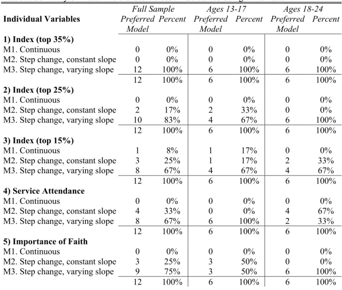
Table 9 provides a summary of model preferences for each of the five religion variables
across both age groups. The most significant finding is that the linear-only model (Model 1) is
only preferred once out of 60 possible combinations (2 percent). Model 2, which contains a
dummy variable for high values, is preferred 12 times (20 percent). Model 3, containing both the
dummy variable and the interaction, is preferred 47 times, or 78 percent. This pattern holds after
dividing these results into the two age groups of interest. In fact, there does not appear to be a
clear preference for non-linear models in one age group compared to the other. Rather, with the
exception of one instance for 13-17 year-olds, all of the preferred models for both age groups are
non-linear models. Model 2 is preferred equally among groups – 6 times each – and Model 3 is
preferred 23 and 24 times, respectively, among the groups. Models without control variables
have not been presented here (available upon request), but the findings are highly consistent with
the general conclusions and preferences discussed thus far. In other words, the non-linear
influence of religious variables is not explained away by the control variables included here.
For the religiosity index, labeling the top 15, 25, or 35 percent of individuals' scores as
highly religious does not change the preference for non-linearity, but it does seem to matter for
distinguishing between Models 2 and 3 (a step change with a constant slope versus a step change
with a varying slope). The top 35 percent threshold for high religiosity exhibits a preference for
Model 3 for all dependent variables in either age group. The top 25 and 15 percent groups do not
service attendance favors Model 3 for the younger sample, interestingly, but predominately
favors Model 2 for the older sample. The importance of faith has nearly the opposite pattern;
Models 2 and 3 are equally preferred for the younger sample, but the varying slope, Model 3, is
preferred for all six cases among the older sample.
The results presented here provide evidence in support of two of the three hypotheses.
The first hypothesis, which states that these relationships will be governed by a threshold effect,
is supported by both significant dummy variables for high religiosity and by significant
interaction terms for high religiosity across the models. While these terms are not always
significant, the results from Table 9 show that accounting for this threshold improves the
linear-only modeling approach for all but one case. The second hypothesis states that religious
variables will function as non-linear predictors when the threshold between low and high
religiosity distinguishes between 15 and 35 percent of youth as highly religious. Again, this
appears to be the case, and Table 9 provides evidence that a threshold at any one of these three
values is associated with non-linearity that is more effectively modeled by allowing the highly
religious to be different from their peers. Lastly, the third hypothesis states that the previously
mentioned threshold effects for religious variables will be more pronounced during young
adulthood than during adolescence. For all combinations of independent and dependent variables
presented here, the non-linearity of these relationships is pervasive enough that there do not
appear to be differences. In fact, there is only one instance in which a non-linear model is not
preferred, and thus the non-linearity of religious variables seems to be equally as prominent
DISCUSSION
The functional forms of religious influence have heretofore been given little attention. As
a result, religious variables have predominately been conceptualized and used as continuous,
linear measures in previous research. The primary argument of this paper is that such an
approach could be masking non-uniformities of religious influence. Specifically, there are
theoretical reasons to believe, and empirical data to suggest, that the most religious individuals
may be distinct enough from their peers to warrant special analytical attention. For these
individuals, religious influence might operate differently than for the rest. To test this idea here,
five religious variables have been used to predict six different outcomes with three different
functional forms.
The primary finding from these analyses is that continuous measures of religiosity rarely
provide the optimal functional form. In fact, across six dependent variables of interest, a
linear-only version of the independent variables produces the preferred model linear-only once. Allowing an
additional effect for being "highly religious" improves many linear-only models and is preferred
about 20 percent of the time. However, the best approach seems to be allowing religiosity to
have a different slope for those highest in religiosity. This most often produces the best model –
about 78 percent of the time in these analyses. These findings hold with and without controls,
meaning that control variables do not explain away the non-linearity.
Instead of conceptualizing religious influence as monotonic, then, religious influence
should perhaps be re-conceptualized to accommodate the theory and evidence presented here.
For example, the functional form that best fits about one fifth of the models here has been
described as a step change with a constant slope. For these models, it is group membership
threshold into “high” religiosity, religious influence is modest – if even present at all. After this
point, additional gains in religiosity do not improve the predictive power of religion. One
rationale for this conceptualization regards religious programs, institutions, and peer groups.
Even the least religious individuals within the “highly” religious group will likely be protected
against risky sexual activity, for example, if only because they are surrounded by institutions,
peers, and parents that are monitoring them and providing alternative opportunities for them to
engage in (Adamczyk 2009; Adamczyk and Felson 2006, 2012).
Conceptually and analytically, another functional form may be even more useful, though.
The form that garners the most support from the findings here is that with a step change and
varying slope. That is, the returns to increases in religiosity are markedly different for those
above and below the high religiosity threshold. For those below it, increases in religiosity vary
from having no influence to a modest influence, depending on the outcome. This could be
visualized as a fairly flat line. For those above the threshold, increases in religiosity make large
differences in their lives, as if the slope of that line takes a sharp turn upward or downward. Not
only do these individuals benefit from entry into “high” religiosity, but the more religious they
become, the more it seems to make a difference. This is consistent with the idea that identities
and schemas, especially when given opportunity for enactment and material resources, can be
reinforced and strengthened over time (Johnson-Hanks et al. 2011; Smith 2003; Stryker 1968).
Unfortunately, the results here do not speak to the mechanisms through which religion is
operating. Whether the highly religious youth in the present sample are benefitting from the nine
factors outlined by Smith (2003), have a salient religious identity (Stryker 1968), or have
religious schemas guiding their attitudes and behaviors (Johnson-Hanks et al. 2011) is hard to